Munich Personal RePEc Archive
A conditional full frontier approach for
investigating the Averch-Johnson effect
Halkos, George and Tzeremes, Nickolaos
University of Thessaly, Department of Economics
December 2011
Online at
https://mpra.ub.uni-muenchen.de/35491/
A conditional full frontier approach for investigating the
Averch-Johnson effect
by
George E. Halkos and Nickolaos G. Tzeremes
Department of Economics, University of Thessaly, Korai 43, 38333, Volos, Greece
Abstract
This paper applies a probabilistic approach in order to develop conditional and unconditional Data Envelopment Analysis (DEA) models for the measurement of sectors’ input oriented technical and scale efficiency levels for a sample of 23 Greek manufacturing sectors. In order to capture the Averch and Johnson effect (A-J effect), we measure sectors’ efficiency levels conditioned on the number of companies competing within the sectors. Particularly, various DEA models have been applied alongside with bootstrap techniques in order to determine the effect of competition conditions on sectors’ inefficiency levels. Additionally, this study illustrates how the recent developments in efficiency analysis and statistical inference can be applied when evaluating the effect of regulations in an industry. The results reveal that sectors with fewer numbers of companies appear to have greater scale and technical inefficiencies due to the existence of the A-J effect.
Keywords: Averch-Johnson effect; Industry regulations; Manufacturing sectors; Nonparametric analysis.
1. Introduction
Regulatory actions on monopoly firms and deregulatory actions towards
competitive markets are two interrelated issues which have been addressed
extensively by the literature in the scope of capital utilization (Kim 1999). The most
frequently used regulations are the rate-of-return and the price-cap (Blank and Mayo
2009). The regulations are imposed by a regulatory agency often prompted by a court
(Sherman 1985). In theory, a regulatory agency targets to improve general welfare by
imposing regulations in order to correct market anomalies but this may not always be
the case (Klevorick 1966). Joskow (2005) provides different results derived from
regulation and deregulation cases. Sectors like airlines, railroads, electric power, gas
and oil were imposed with some sort of regulation. The process of deregulation has
been completed in a number of cases while in other cases the deregulation process is
on-going.
In their seminal work, Averch and Johnson (1962) study a monopoly firm
which seeks to maximize its profits under rate-of-return regulation. The monopoly
firm employs capital and labor to produce one output. The availability of capital and
labor is assumed to be unlimited and the price per unit fixed. The regulatory agency
imposes a “fair rate of return” on the firm through the rate-of-return regulation. If the
firm’s unrestricted rate of return is smaller than the “fair rate of return” then the firm
is allowed to act as if there was no regulation and for example raise the price.
Otherwise if the firm’s unrestricted rate of return is bigger than the “fair rate of
return” then the firm will be compelled to lower the price. After that, according to the
Averch-Johnson effect (A-J effect) and under the assumption of no regulatory lags
(Johnson, 1973), if the cost of “fair rate of return” is greater than the cost of capital
where the capital-labor ratio is not optimum. Although the firm will not minimize the
cost of production, the excessive use of capital will allow the firm to achieve greater
profits through a bigger “fair rate of return”.
Our paper applies for the first time conditional full frontiers, based on the
probabilistic approach of efficiency measurement developed by Daraio and Simar
(2005, 2007a, 2007b) and in order to investigate the A-J effect for the Greek
manufacturing sectors. Furthermore it applies the statistical inference framework
developed by Simar and Wilson (1998, 2000a, 2000b) on the conditional efficiency
measures obtained in order to create biased free estimates. The structure of the paper
is the following. Section 2 presents the literature review, while section 3 discusses the
data used and the proposed methodology. Section 4 comments on the empirical results
derived while the last section concludes the paper.
2. A brief review of the literature
Takayama (1969) following the study by Averch and Johnson (1962)
presented an alternative mathematical formulation of the problem and obtained
similar results about the overcapitalization of a regulated monopolistic firm. In
addition, Westfield (1965) examined the possibility of conspiracies among buyers and
sellers of plant, machinery and electrical equipments. He demonstrated that a private
power generating company which is under regulation is willing to pay more for the
capital equipment. This capital waste can lead the monopoly firm to achieve greater
profits. Klevorick (1966) suggested an inverse relation among the “fair rate of return”
and amount of capital employed in order to deal with the A-J effect. Thus, if the firm
raises its capital, the “fair rate of return” will be reduced.
Furthermore, Stigler and Friedland (1962) are the first to investigate A-J effect
without regulations. In addition, Spann (1974) applied a translog production function
in order to study the regulated electric utilities. He relied on Stigler and Friedland
(1962) study where the effect of regulation is assumed to be uniform across the states,
and allows the effect to vary. The results appeared to verify the A-J effect.
Additionally, the A-J effect is validated by Petersen (1975) who marks that a more
tightened regulation leads to an increase of the firm’s unit costs.
Moreover, Sherman (1972) notes that rate-of return regulation will drive the
firm to continue behaving as a monopoly for every input except capital, but it will
make choices about capital as if it was in a competitive market. The rate-of-return
regulation has additional negative effects which in fact may be more significant than
input distortions, like the absence of motivation for innovative actions and efficient
operation. Another negative effect of rate-of-return regulation is the technological
advancement and R&D (Frank 2003a).
Rumbos (1999) introduced the variable utilization rate of capital stock in the
profit maximization problem of the monopolistic firm and proposed the measurement
of the inefficiency of the production of total services of capital instead of the ratio of
capital and labor. On the other hand, Maloney (2001) employed a variable cost
function in order to measure electricity generation industry. In addition, Kolpin (2001)
introduces a dynamic model, which incorporates among others, multiple inputs and
outputs, periods of production and uncertainty, in order to test and verify the A-J
effect. Finally, Caputo and Partovi (2002) defined four conditions under which the
A-J effect is present.
A number of authors challenge the traditional assumptions and results of the
A-J effect. Baumol and Klevorick (1970) argued that in practice regulatory lags exist.
time period. Also, the authors note that every tax leads to input distortion and
rate-of-return regulation has not an additional effect in practice. Zajac (1970) exhibited the
geometrical presentation of the A-J effect and questioned some of the original
model’s assumptions. Among others, the author came in line with Baumol and
Klevorick (1970) about regulatory lags and he has found no solid evidence about the
regulated monopolistic firms’ optimum strategy between the minimization of the cost
or the overcapitalization.
One of the most famous cases of a regulated monopolistic firm is in the US
telephone industry, the American Telephone and Telegraph Company (AT&T). Irwin
(1997) presented the internal story of the investigation about the firm. The author
provided evidence that the AT&T was purchasing the equipment from Western
Electric in a very high price, confirming the A-J effect in practice. The natural
monopoly of AT&T was ended in 1984 when the company was divested from the Bell
operating companies, a move which is now considered as a pro-competitive change
(Ying and Shin 1993). Oum and Zhang (1995) investigated the US telephone industry
after the transformation towards competition. The authors find evidence that
introduction of competition has increased productive efficiency and reduced A-J
effect.
They also demonstrated that introducing competition in a previously regulated
monopolistic industry may result in multiple benefits like innovations and improved
quality. In general, competition appears to be the solution in order to reduce
inefficiencies from monopoly and especially regulated monopoly. Dixon and Easaw
(2001) studied the UK gas industry for the period 1986-1996 including the
privatization period. The authors argue that competition is necessary in order to
heteroscedastic stochastic frontier models for the Greek bank sector found evidences
that increased competition after the privatization period reduced the allocative and
technical inefficiencies associated with the previous regulated industry conditions.
Frank (2003b) investigated the electric utilities in Texas for the period
1965-1985, ten years before and ten years after the rate-of-return regulation. He has found
that before 1975 technological progress results in decreasing costs while after 1975
the negative effect of regulation on technological progress results in greater costs.
Finally, in contrast to the previous mentioned studies examining separate
sectors and different industries’ competitive conditions, our study for the first time
applies a different approach analysing twenty three manufacturing sectors based on
the new advances of efficiency analysis as has been introduced by several authors
(Daraio and Simar 2005, 2007a, 2007b; Bădin et al. 2010; Jeong et al. 2010) and in
order to investigate the A-J effect.
3. Data and Methodology
3.1 Data description
Our analysis uses data of the Greek manufacturing sector as has been provided
from ICAP (2007). The data are based on the balance sheets of income statements of
2006. More analytically, consolidated income statements of every Greek
manufacturing sector have been used for the companies which are listed in Athens
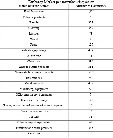
Stock Exchange. In addition table 1 provides a description of the manufacturing sector
alongside with information regarding the number of companies competing in each of
them. In our analysis and in order to model in a nonparametric context the A-J effect
the number of companies in a sector are used as a proxy of the competitive structure
‘tobacco products’, ‘office machinery, computers’ and ‘recycling’ are the sectors with
the lowest competition and oligopoly conditions where as the sectors of ‘food and
beverages’, ‘non-metallic mineral products’ and ‘Publishing-printing’ appear to have
increased competition.
In terms of the Data Envelopment Analysis (DEA) context the measurement of
each sector’s efficiency levels must be measured after defining the proper
inputs/outputs. Since the A-J effect describes that monopoly firms tend to use more
capital than the economic efficient level in order to produce their outputs (Averch and
Johnson, 1962), this study uses total assets and inventories (measured in thousands of
€) as the two inputs. In addition the outputs used are sales and gross profit levels (also
measured in thousands of €).
Table 2 provides the descriptive statistics of the variables used. As it is
revealed from the high standard deviation values there are several dissimilarities
among the sectors indicating the different nature and structure of the sectors under
examination. Since the efficient input utilisation is the subject of the A-J effect, our
DEA formulation uses input orientation due to the fact that that input quantities
appear to be the primary decision variables (Coelli et al. 2005). In our DEA context
the input-oriented technical efficiency is used enabling us to model the ability of the
sectors to use minimum input quantities given their level of output quantities.
Finally, by applying the methodology introduced by Daraio and Simar (2005,
2007a, 2007b) we conditioned in a second stage analysis the effect of competition on
sectors’ input–oriented technical efficiency levels. As explained earlier the number of
companies competing in every sector has been used as an external variable in our
Table 1: Number of companies listed in the Athens Stock Exchange Market per manufacturing sector
Manufacturing Sectors Number of Companies
Food-beverages 1,214
Tobacco products 4
Textile 301
Clothing 369
Leather 73
Wood 125
Paper 127
Publishing-printing 459
Oil refining 31
Chemicals 286
Rubber-plastic products 316 Non-metallic mineral products 500
Basic metals 94
Metal products 457
Machinery, equipment 278 Office machinery, computers 9
Electrical machinery 120 Radio, television and communication equipment 36
Precision instruments 54
Vehicles 31
Other transport equipment 63 Furniture and other products 336
Recycling 10
Table 2: Descriptive statistics of the variables used
Number of Companies
Total Assets (1000 €)
Inventories (1000 € )
Sales (1000 €)
Gross Profits (1000 €)
Mean 230.130 2481699.174 415794.826 2002898.130 432042.304 Std 269.213 3068654.956 472310.005 2769825.576 643519.695 Max 1214.000 14150226.000 1919614.000 10061793.000 2839887.000
[image:9.595.89.436.583.690.2]3.2 DEA models and bias correction
Following the notation from Daraio and Simar (2007a), Koopmans (1951) and
Debreau (1951) definition of production technology can be characterized as a set of
p
R
x inputs which are used to produce yRq outputs. Then the feasible
combinations of
x, can be defined as: y
x can produce y
R y
x, p q
(1)
By assuming free disposability of inputs and outputs then
x y, and at the same time
x y', '
when x x' and y' y. As suggested by several authors(Førsund and Sarafoglou 2002; Førsund and Sarafoglou 2005; Førsund et al. 2009),
Hoffman’s (1957) discussion regarding Farrell’s (1957) paper was the first to indicate
that linear programming can be used in order to find the frontier and estimate
efficiency scores, but only for the single output case. Later, Boles (1967) developed
the formal linear programming problem with multiple outputs identical to the constant
returns to scale (CRS) model in Charnes et al. (1978) who named the technique as
Data Envelopment Analysis (DEA). Later, Banker et al. (1984) introduced a DEA
estimator allowing for variable returns to scale (VRS model)1.
As such, based on the Farrell (1957) measure for a unit operating at the level
x y, the input oriented efficiency score can be defined as:
x y, inf
x y,
(2)
1For information regarding the history of the origins of efficiency measurements see Cooper and
Then the efficiency measurement of a given country ( , )x yi i defines an individual
production possibilities set
x yi, i
, which under the assumption of freedisposability of inputs and output can be expressed as:
,
, p q ,
i i i i
x y x y x x y y
(3).
As such the union of these individual production possibilities sets provides the
Free Disposal Hull (FDH) estimator (introduced by Derpins et al. 1984) of the
production set which can be written as:
1 , , , , 1,...,
n
p q
FDH i i i i
i x y x y x x y y i n
(4)
It follows that the DEA estimator2
DEA
is obtained by the convex hull (CH)
of FDH
and can be calculated as:
1 1 1 1 1 , , ;,..., . . 1; 0, 1,...,
n
DEA i i i
n n
p q
i i i i
i i
n
n i i
i
CH x y
x y y y x x
for s t i n
(5)Next and in order to obtain the corresponding input oriented DEA estimators
of efficiency scores we need to incorporate DEA
in equation (2). In addition by
applying the methodology introduced by Simar and Wilson (1998, 2000a, 2000b) we
perform the bootstrap procedure for DEA estimators in order to obtain biased
corrected results (see the Appendix for details). The main applications of bootstrap
(Simar and Wilson 1998; 2000a; 2000b), test procedures to assess returns to scale
(Simar and Wilson 2002), the criterion for bandwidth selection (Simar and Wilson
2002; 2008), statistical procedures for comparing the efficiency means of several
groups (Simar and Wilson 2008), statistical procedures for testing the equality of
distribution of the efficiency scores (Simar and Zelenyuk 2006) and for statistical
inference for aggregate efficiency measures (Simar and Zelenyuk 2007)3.
Thus, following Simar and Wilson (1998, 2000a, 2000b) procedure the bias
corrected efficiency score is given by:
1
, 1
( , ) ( , ) ( , ) 2 ( , ) B * ( , )
DEA DEA B DEA DEA DEA b b
x y x y bias x y x y B x y
(6)After that and by expressing the input oriented efficiency in terms of the Shephard
(1970)) input distance function as ( , ) 1 ( , )
DEA
DEA
x y
x y
we can construct bootstrap
confidence intervals for DEA( , )x y
as:
1 / 2 / 2
( , ) a , ( , ) a D EA x y D EA x y
(7).
Furthermore, following the bootstrap test developed by Simar and Wilson
(2002) we test whether the CRS or VRS formulation is appropriate in our analysis.
The null hypothesis of the test can be developed as
:
0
H is globally CRS against :
1
H is VRS.
Subsequently the test statistic mean of the ratios of the efficiency scores is provided
by:
2We consider here only the VRS case; however CRS can be obtain by dropping the constraint in (5)
n i i i n VRS i i n CRS n Y X Y X n X T 1 , , ) , ( ) , ( 1 ) ( (8).Similarly, the p-value of the null-hypothesis can be obtained as:
) )
(
(T X T H0 is true
prob value
p n obs (9)
where Tobs is the value of T computes on the original observed sample Xn. It follows
that the p-value can be approximated by the proportion of bootstrap values of T*b less
the original observed value of Tobs such as:
B b obs b B T T value p 1 * (10).3.3 Calculating the conditional measures of efficiency
Daraio and Simar (2005, 2007a, 2007b) by extending the ideas developed by
Cazals et al. (2002) developed a probabilistic formulation of the production process.
This probabilistic approach allowed the introduction of external-environmental factors
(Z) directly in the production process4. In contrast to the traditional two-stage approaches, the probabilistic approach introduced by Daraio and Simar (2005, 2007a,
2007b) does not impose a reparability assumption between Z values and the
input-output space (De White and Verschelde 2010)5. By denoting Zr as the external
3 For an empirical application of bootstrapped DEA investigating firms’ and sectors’ efficiency levels
see Halkos and Tzeremes (2010, 2011)
4For the theoretical background of the statistical properties of the conditional estimators see Jeong et
al. (2010).
factors, the joint distribution of
X Y,
conditional on Z z defines the production process if Z z . In this way the attainable production set zis defined by:
, , Prob ,
X Y Z
H x y z X x Y y Z z (11).
Then the input oriented conditional efficiency measure can be defined as:
, , F , ,
X Y Z X Y Z Y Z
H x y z x y z S y z (12).
In addition the input oriented efficiency score can be obtained from:
, 0
inf ) ,
(x yz FX xy z
(13).
It follows that a kernel estimator can be calculated as:
y y
K
z z
h
I h z z K y y x x I z y x F i n i i n
i i i i
n Z Y X / / , , 1 1 , ,
(14)where K(.) is the Epanechnikov kernel6 and h is the bandwidth of appropriate size.
Following, Bădin et al. (2010) we use a fully automatic data-driven approach
for bandwidth selection based on the work of Hall et al. (2004) and Li and Racine
(2004; 2007) least-squares cross-validation criterion (LSCV) which leads to
bandwidths of optimal size for the relevant components of Z. This method is based
on the principle of selecting a bandwidth that minimizes the integrated squared error
of the resulting estimate7. Li and Racine (2007) suggest that we have also to correct
the resulting h by an appropriate scaling factor, which equals to 4 4
q q r r
n
where
6Other kernels from the family of continuous kernels with compact support can also be used.
7 See Bădin et al. (2010) for a Matlab routine that computes the bandwidth based on the LSCV
qis the dimension of Y and ris the dimension ofZ8. Therefore, we can obtain a conditional DEA efficiency measurement defined as:
0 , inf,yz F , , xy z
x XYZn
DEA
(15).
Then in order to visualize the influence of an environmental variable on the
efficiency scores obtained, a scatter of the ratios
, , n z nx y z Q x y
against z (the number
of companies competing in a sector) and the smoothed nonparametric regression lines
would help us to analyze the effect of Zon the sectors’ efficiency scores obtained. Similarly, the effect of competition on sectors’ scale efficiency can be visualized if we
use a scatter of the ratios
, , , , , , , , , CRS n VRS n Scale z CRS n VRS n
x y z x y z Q x y x y
against z. For this purpose we use the
nonparametric regression estimator introduced by Nadaraya (1965) and Watson
(1964) as: 1 1 ( ) ( ) ( ) n i i n i i z Z K Q h
g z z Z
K h
(16).If this regression line is increasing it indicates that Z is unfavorable to the sectors’ efficiency levels whereas if it is decreasing then it is favorable. When Z is unfavorable then the number of companies acts like an extra undesired output to be
produced demanding the use of more inputs in the production activity. In the opposite
case the external factor plays a role of a substitutive input in the production process
8For more information regarding LSCV criterion and its properties see Silverman (1986), Hall et al.
giving the opportunity to save inputs in the production activity. This of course is very
crucial when investigating the A-J effect.
An increasing regression line in our case will indicate that competition has a
negative effect on sectors utilization of capital, whereas a decreasing line will indicate
that sectors use their inputs in an economical efficient way. Even though the
visualization framework of the effect of the environmental variableZ (Daraio and Simar 2005, 2007a, 2007b) provides us with useful information, it does not give us
any indication of the significance of the observed effect. For that reason our study
adopts a significance test for nonparametric regression as has been introduced by
several authors (Racine 1997; Racine et al. 2006; Li and Racine 2007) in order to
compute a significance level of the observed effect of the external variable on sectors’
input oriented technical efficiency levels.
If the conditional mean E Q z
z
is independent from zthen the vector ofpartial derivatives of E Q z
z
with respect to z will be equal to zero. Thus:
z
0z
E Q z E Q z z
z
(17).
From equation (17) we can derive the null hypothesis as:
0 0
z
E Q z
H g z
z
(18).
In this way the test statistic the estimator of
2
I E g z
and can be
obtained by forming a sample of average of I replacing the unknown derivatives with
i
2 11 n
n i
i
I g z
n
(19).
Finally, the distribution of the statistic can be obtained by applying the bootstrap
procedure described in Racine (1997).
4. Empirical results
Following the methodology proposed by Simar and Wilson (2002) our paper
tests the model for the existence of constant or variable returns to scale. In our
application we have two inputs and two outputs and we obtained for this test a p-value
of 0.028 < 0.05 (with B=2000) implying rejection of the null hypothesis of CRS.
Therefore, the results adopted in our study are based on the BCC model (Banker et al.
1984) assuming variable returns to scale9.
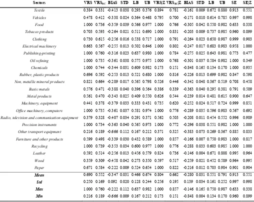
Table 3 provides the results of VRS analysis10 adopting the bias correction
method using the methodology proposed by Simar and Wilson (1998, 2000a, 2000b).
For the sample of 23 manufacturing sectors under the VRS assumption seven sectors
appear to be efficient (efficiency score = 1). These are the sector of ‘Food’,
‘Publishing-printing’, ‘Oil refining’, ‘Chemicals’, ‘Office machinery, computers’,
‘Precision instruments’ and the ‘Recycling’ sector. The last seven performers are
reported to be the sectors of ‘Metal products’, ‘Vehicles’, ‘Machinery and
equipment’, ‘Textile’, ‘Radio, television and communication equipment’, ‘Wood’ and
‘Other transport equipment’.
However, when looking at the bias corrected efficiency results (VRSBC), we
realize that the efficiency scores are in many cases considerably lower. For instance in
9 Due to size inequalities among the Greek manufacturing sectors the most appropriate assumption for
the case of the ‘Food’ sector the biased corrected (BC) efficiency score is 0.736
(original VRS score equals to 1) with lower bound (LB) of 0.566 and upper bound
(UB) of 0.977 in a confidence interval of 95%. Almost identical results are reported in
the case of ‘Office machinery, computers’ where the biased corrected (BC) efficiency
score is 0.735 with a lower bound (LB) of 0.581 and an upper bound (UB) of 0.974 in
a confidence interval of 95%. Daraio and Simar (2007) suggest that when the bias
(BIAS) is larger than the standard deviation (STD) then the bias corrected efficiencies
[image:18.595.47.555.363.767.2](BC) must be preferred compared to the original estimates.
Table 3: Results of the conditional and unconditional measures of the original and the biased corrected efficiency scores.
Sectors VRS VRSBC BIAS STD LB UB VRS|Z VRSBC|Z BIAS STD LB UB SE SE|Z
Textile 0.384 0.331 -0.413 0.038 0.293 0.376 0.894 0.781 -0.161 0.009 0.672 0.880 0.913 0.551
Vehicles 0.478 0.412 -0.338 0.024 0.364 0.468 0.795 0.700 -0.171 0.010 0.614 0.785 0.997 0.998
Food 1.000 0.736 -0.359 0.039 0.566 0.977 1.000 0.766 -0.305 0.042 0.550 0.982 0.633 0.338
Tobacco products 0.703 0.593 -0.264 0.021 0.511 0.690 1.000 0.831 -0.203 0.009 0.737 0.985 0.960 0.899
Clothing 0.730 0.615 -0.256 0.016 0.538 0.717 1.000 0.791 -0.264 0.023 0.650 0.987 0.999 0.903
Electrical machinery 0.663 0.567 -0.255 0.013 0.502 0.646 1.000 0.802 -0.247 0.017 0.683 0.983 0.958 1.000
Publishing-printing 1.000 0.760 -0.316 0.023 0.637 0.980 1.000 0.784 -0.275 0.025 0.643 0.981 0.773 0.477
Oil refining 1.000 0.735 -0.361 0.038 0.575 0.975 1.000 0.768 -0.301 0.037 0.584 0.982 1.000 0.349
Chemicals 1.000 0.744 -0.344 0.031 0.609 0.982 0.173 0.151 -0.848 0.165 0.134 0.170 1.000 0.935
Rubber, plastic products 0.696 0.592 -0.253 0.013 0.521 0.680 1.000 0.816 -0.226 0.013 0.699 0.982 0.847 0.598
Non, metallic mineral products 0.821 0.664 -0.289 0.017 0.565 0.798 0.526 0.446 -0.342 0.048 0.367 0.519 0.708 0.458
Basic metals 0.576 0.471 -0.388 0.040 0.396 0.564 0.386 0.339 -0.363 0.040 0.295 0.381 0.791 0.509
Metal products 0.561 0.470 -0.343 0.025 0.409 0.550 0.626 0.544 -0.239 0.014 0.481 0.615 0.900 0.647
Machinery, equipment 0.441 0.378 -0.379 0.033 0.333 0.431 0.735 0.620 -0.252 0.024 0.517 0.724 0.999 0.851
Office machinery, computers 1.000 0.735 -0.361 0.037 0.581 0.974 1.000 0.776 -0.289 0.035 0.596 0.983 0.567 0.692
Radio, television and communication equipment 0.379 0.328 -0.407 0.034 0.291 0.371 0.562 0.503 -0.208 0.011 0.454 0.552 0.996 0.989
Precision instruments 1.000 0.734 -0.363 0.040 0.565 0.973 1.000 0.772 -0.296 0.038 0.551 0.982 1.000 1.000
Other transport equipment 0.216 0.189 -0.666 0.112 0.167 0.212 0.371 0.325 -0.383 0.073 0.269 0.367 0.885 0.833
Furniture and other products 0.599 0.498 -0.339 0.030 0.432 0.589 1.000 0.857 -0.166 0.007 0.750 0.983 1.000 0.817
Recycling 1.000 0.739 -0.353 0.034 0.600 0.977 1.000 0.776 -0.288 0.033 0.603 0.985 1.000 1.000
Leather 0.592 0.514 -0.256 0.013 0.456 0.579 0.824 0.736 -0.146 0.004 0.671 0.808 0.995 0.964
Wood 0.359 0.309 -0.458 0.042 0.273 0.350 0.597 0.517 -0.259 0.021 0.452 0.589 0.964 0.995
Paper 0.671 0.584 -0.222 0.009 0.524 0.654 1.000 0.822 -0.216 0.012 0.703 0.984 0.901 0.904
Mean 0.690 0.552 -0.347 0.031 0.466 0.674 0.804 0.662 -0.280 0.031 0.551 0.791 0.913 0.551
Std 0.250 0.169 0.092 0.020 0.128 0.244 0.256 0.195 0.139 0.034 0.161 0.252 0.997 0.998
Max 1.000 0.760 -0.222 0.112 0.637 0.982 1.000 0.857 -0.146 0.165 0.750 0.987 0.633 0.338
In addition table 3 provides the analytical results obtained following the
conditional measurement approach by Daraio and Simar (2005, 2007a, 2007b) and the
statistical inference framework by Simar and Wilson (1998, 2000a, 2000b) in order to
measure sectors’ efficiency when accounting for the effect of the number of
companies competing within a sector. According to De White and Marques (2007, p.
25) integrating these two frameworks can help us to avoid main drawbacks of
efficiency analysis and have some attractive features such as
1) The absence of separability condition,
2) The avoidance of the need for priory assumptions on the functional form of
the model and
3) The allowance of the exploration of the effect of environmental variables.
Furthermore, table 3 presents the results estimated from the conditional
measures under the VRS assumption taking into account the effect of the number of
companies competing within a sector (VRS|Z). The results indicate that twelve sectors
appear to be efficient. These are ‘Food’, ‘Publishing-printing’, ‘Oil refining’, ‘Office
machinery, computers’, ‘Precision instruments’, ‘Recycling’, ‘Clothing’, ‘Tobacco
products’, ‘Rubber, plastic products’, ‘Paper’, ‘Electrical machinery’ and ‘Furniture
and other products’.
However as previously stated the biased corrected results need to be adopted
(VRSBC|Z) since the bias is larger than the standard deviation (Daraio and Simar
2007a). Again great differences are reported between the biased corrected and the
original conditional efficiencies. Taking into consideration these biased corrected
conditional efficiency scores the highest five performers in a descending order are
reported to be ‘Furniture and other products’, ‘Tobacco products’, ‘Paper’, ‘Rubber,
lowest biased corrected conditional efficiency scores are reported to be ‘Radio,
television and communication equipment’, ‘Non metallic mineral products’, ‘Basic
metals’, ‘Other transport equipment’ and ‘Chemicals’.
Finally, the last two columns of table 3 report the original and the conditional
scale efficiency scores. The top five performers of scale efficiencies are ‘Chemicals’,
‘Clothing’, ‘Oil refining’, ‘Furniture and other products’ and ‘Machinery, equipment’.
Under the conditional measures the top five performers of scale efficiencies are
‘Electrical machinery’, ‘Clothing’, ‘Vehicles’, ‘Radio, television and communication
equipment’ and ‘Wood’. According to Balk (2001, p.168) increased scale efficiency
means that the sector has moved to a position with a better input-output quantity ratio
at the frontier.
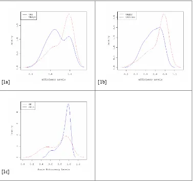
In addition, Figure 1 presents the density estimates using the “normal
reference rule-of-thumb” approach for bandwidth selection (Silverman 1986) and a
second order Gaussian kernel. Subfigure 1a, indicates the differences between sectors’
input oriented technical efficiency scores against the conditional input oriented
technical efficiency scores (VRS|Z). It appears that the original estimates under the
VRS assumption (solid line) are platykurtic compared to the original VRS conditional
estimates (dotted line) which appear to be leptokurtic. The leptokurtic distributions
indicate that there is a rapid fall-off in the density as we move away from the mean.
Furthermore, the pickedness of the distribution suggests a clustering around
the mean with rapid fall around it. In addition subfigure 1b indicates high differences
between the densities of the biased corrected efficiency scores (VRSbc-solid line) and
the biased corrected conditional efficiency scores (VRS|Zbc-dotted line). As can be
realised the conditional estimates (original and biased corrected) are reported to show
biased corrected). This in turn indicates that when we account for the effect of
competition on sectors’ efficiency scores, this results on increasing sectors’ efficiency
levels. Moreover, subfigure 1c indicates the differences between sectors’ original and
conditional scale efficiencies. As can be realized the unconditional scale efficiencies
are leptokurtic, whereas the conditional scale efficiencies are platykurtic. Finally, it
appears that the original scale efficiencies are higher compared to the conditional
[image:21.595.87.464.347.700.2]ones.
Figure 1: Kernel density functions of sectors’ efficiencies derived from unconditional and conditional VRS and biased corrected VRS DEA models using Gaussian Kernel and the appropriate bandwidth
[1a] [1b]
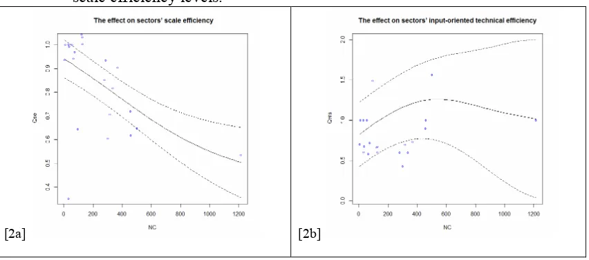
In these lines, Figure 2 provides a graphical representation of the effect of the
number of companies on sectors’ input oriented technical and scale efficiency. For
this task we use the ‘Nadaraya-Watson’ estimator, which is the most popular method
for nonparametric kernel regression proposed by Nadaraya (1965) and Watson (1964).
For both the cases the significance of the effect of Z (number of companies –NC) in
the nonparametric regression setting was based on the procedure described previously
(Racine 1997; Racine et al. 2006; Li and Racine 2007). For the scale efficiencies a
value of 0.029 was attained, while for the input orientated technical efficiencies a
p-value of 0.032 was obtained, indicating significance at 5% level.
As such subfigure 2a illustrates the nonparametric estimate of the regression
function using the conditional and unconditional biased corrected scale efficiency
estimates. Moreover it presents their variability bounds of point wise error bars using
asymptotic standard error formulas (Hayfield and Racine 2008). When the regression
is decreasing, it indicates that ‘Z’ factor (i.e. the number of companies competing
within a sector) is favorable to sector’s scale efficiency levels. In our case subfigure
2a illustrates a decreasing nonparametric regression line indicating that the high
number of companies competing within a sector increase sector’s scale efficiency
levels. Therefore, the number of companies acts as a substitutive input in the
production process of sectors’ scale efficiency providing the opportunity to “save”
inputs in the activity of production.
In addition when we looking at subfigure 2b the regression line has a steeper
and increasing shape for a lower number of firms competing within a sector,
indicating a highly negative effect on sectors’ input oriented technical efficiency
levels. However, for higher number of companies the regression line has a decreasing
by Christopoulos and Tsionas (2001) indicating that during the deregulation period
the Greek banking sector decreased its allocative and technical inefficiencies. In
addition they have reported that through the intensification of cross-country
competition the efficiency has been increased.
Finally, our results confirm the findings of Oum and Zhang (1995) indicating
that increased competition affects positively firms to use efficiently their capital
inputs and therefore to reduce the allocative inefficiency caused by the A-J effect.
Therefore it appears that Greek manufacturing sectors with higher competition tend to
have higher scale and input oriented technical efficiency levels compared with the
sectors with monopolized/oligopolized conditions which induce an economically
[image:23.595.87.513.454.642.2]inefficient use of capital.
Figure 2: The global effect of competition on sectors’ input-oriented technical and scale efficiency levels.
5. Conclusions
This paper applies the probabilistic approach in a sample of 23 Greek
manufacturing sectors and in order to construct conditional efficiency measures taking
into account the effect of competitive conditions within the sectors. Then by applying
an inferential approach on DEA efficiency scores it measures the bias corrected
sectors’ input oriented technical efficiency levels. Furthermore, the biased corrected
results and 95% confidence intervals have been produced indicating major
inefficiencies among the sectors.
At a second stage of the analysis our paper uses nonparametric regressions in
order to quantify the effect of competitive conditions on sectors’ scale and input
oriented technical efficiency levels by calculating their conditional measures. In
addition and in order to establish if the effect is statistical significant, our paper
applies a nonparametric statistical test. The results reveal that the increased
competition has a positive effect on sectors’ scale and input oriented technical
efficiency levels reducing the inefficiencies caused by the A-J effect.
Finally our contribution to the existing literature with respect to the
methodology used is that we provide evidence of how the new advances and recent
developments in efficiency analysis and statistical inference can be applied and
directed towards an effective evaluation of industrial policies, providing in such a way
a vital tool to industrial policy makers for analyzing the effects of their policies on
industry regulation problems.
Acknowledgements
APPENDIX
This appendix synoptically illustrates the bootstrapped based algorithm introduced by
Simar and Wilson (1998, 2000a, 2000b). Specifically, the following steps are
followed:
Step 1: Transform the input-output vectors using the original efficiency estimates
n i
in, 1,...,
as
i in i i l
i y x y
x , ,
Step 2: Generate smoothed resampled pseudo-efficiencies *
i
as follows:
2.1 Given a set of estimated efficiencies
in
, use the “rule of thump” (Silverman,
1986, p.47-48) to obtain the bandwidth parameter has
34 . 1 / , min 9 .
0 n1/5 R13
h , where
= the standard deviation of
in
and R13
is the interquartile range of the empirical distribution of
in .
2.2 Generate
*i
by replacing, with replacement, from the empirical distribution of
in
of the estimated efficiencies.
2.3 Generate the sequence ~* i using: otherwise ) ( 2 1 if * * * * * * * ~ i i i i i i i h h h
where *
i
2.4 Generate thesmoothed pseudo-efficiencies
*i
using the following formula:
n
i i i
i i i
i h 1 * n
* 2 2 * * ~ *
* ( )/ 1 / ,where /
which is the average of the
resampled original efficiencies.
Step 3: Let the pseudo-data be given by
li i i i
i y x y
x*, * /*,
Step 4: Estimate the bootstrap efficiencies using the pseudo-data as:
n i n i i i z SWin y Yz x X z z z R
1 * , * ,1 , , :
min
Step 5: Repeat steps (2)-(4) B times to create a set of Bbank specific bootstrapped
efficiency estimates i n b B
b SW
in , 1,..., , 1,..,
*
, According to Simar and Wilson (1998,
REFERENCES
Averch, H. & Johnson, L.L. (1962). Behavior of the firm under regulatory constraint.
American Economic Review, 52(5), 1052-1069.
Bădin, L., Daraio, C. & Simar, L. (2010). Optimal bandwidth selection for conditional
efficiency measures: A Data-driven approach. European Journal of Operational
Research, 201, 633-640.
Balk, B.M. (2001). Scale efficiency and productivity change. Journal of Productivity Analysis, 15, 159-183.
Banker, R.D., Charnes, A. & Cooper, W.W. (1984). Some Models for Estimating
Technical and Scale Inefficiencies in Data Envelopment Analysis. Management
Science, 30, 1078 – 1092.
Baumol, W.J. & Klevorick, A.K. (1970). Input choices and rate-of-return regulation: An overview of the discussion. Bell Journal of Economics, 1(2), 162-190.
Blank, L. & Mayo, J.W. (2009). Endogenous regulatory constraints and the emergence of hybrid regulation. Review of Industrial Organization, 35, 233-255.
Boles, J.N. (1967). Efficiency squared—efficient computation of efficiency indexes. In: Proceedings of the thirty ninth annual meeting of the western farm economics association, pp 137–142.
Caputo, M.R. & Partovi, M.H. (2002). Reexamination of the A-J effect. Economics
Bulletin, 12(10), 1-9.
Cazals, C., Florens, J.P. & Simar, L. (2002). Nonparametric frontier estimation: a robust approach. Journal of Econometrics, 106, 1-25.
Charnes, A., Cooper, W.W. & Rhodes, L.E. (1978). Measuring the efficiency of decision making units. European Journal of Operational Research, 2, 429-444.
Christopoulos, D.K. & Tsionas, E.G. (2001). Banking economic efficiency in the deregulation period: results from heteroscedastic stochastic frontier models.
Manchester School, 69(6), 656-676.
Coelli, T. J., Rao, D. S. P., O'Donnell, C. J. & Battese, G.E. (2005). An Introduction to Efficiency and Productivity Analysis. Second ed. New York: Springer.
Cooper, W.W. & Lovell, C.A.K. (2011). History lessons. Journal of Productivity Analysis, 36(2), 193-200.
Daraio, C. & Simar, L. (2007a). Advanced robust and nonparametric methods in efficiency analysis. Springer Science: New York.
Daraio, C. & Simar, L. (2007b). Conditional nonparametric frontier models for convex and nonconvex technologies: a unifying approach. Journal of Productivity Analysis, 28, 13-32.
De White, K. & Marques, R.C. (2007). Designing incentives in local public utilities, an international comparison of the drinking water sector. Center for Economic Studies, Discussions Paper Series (DPS) 07.32, Department of Economics, UniversitéCatholique de Louvain.
De White, K. & Verschelde, M. (2010). Estimating and explaining efficiency in a multilevel setting: A robust two-stage approach. TIER working paper series, TIER WP 10/04, Top Institute for Evidence Based Education Research, University of Amsterdam, Maastricht University, University of Groningen.
Debreu, G. (1951). The coefficient of resource utilization. Econometrics, 19(3), 273– 292.
Derpins, D., Simar, L. & Tulkensmm H. (1984). Measuring labor efficiency in post offices. In M. Marchand, P. Pestieau & H. Tulkens (Eds.), The performance of public enterprises: Concepts and measurement. Amstredam: North-Holland, pp. 243-267.
Dixon, H. & Easaw, J. (2001). Strategic responses to regulatory policies: What lessons can be learned from the U.K. contract gas market. Review of Industrial Organization, 18, 379-396.
Farrell, M. (1957). The measurement of productive efficiency. Journal of the Royal
Statistical Society Series A, 120, 253–281.
Førsund, F.R. & Sarafoglou, N. (2002). On the origins of data envelopment analysis.
Journal of Productivity Analysis, 17(1/2), 23–40.
Førsund, F.R. & Sarafoglou, N. (2005) The tale of two research communities: the diffusion of research on productive efficiency. International Journal of Production Economics, 98(1), 17–40.
Førsund, F.R. & Sarafoglou, N. (2009). Farrell revisited–Visualizing properties of DEA production frontiers. Journal of the Operational Research Society, 60, 1535-1545.
Frank, M.W. (2003a). The impact of rate-of-return regulation on technological innovation. The Burtun Center for Development Studies, VT: Ashgate Publishing Company.
Halkos, G.E. & Tzeremes, N.G. (2010). The effect of foreign ownership on SMEs performance: An efficiency analysis perspective. Journal of Productivity Analysis, 34, 167-180.
Halkos, G.E. & Tzeremes, N.G. (2011). Industry performance evaluation with the use of financial ratios: An application of bootstrapped DEA. Expert Systems with Applications, doi:10.1016/j.eswa.2011.11.080.
Hall, P., Racine, J.S. & Li, Q. (2004). Cross-validation and the estimation of conditional probability densities. Journal of the American Statistical Association, 99, 1015–1026.
Hayfield, T. & Racine, J.S. (2008). Nonparametric Econometrics: The np Package.
Journal of Statistical Software, 27(5), 1-32.
Hoffman, A.J. (1957). Discussion on Mr. Farrell’s Paper. Journal of the Royal Statistical Society Series A, 120(III), 284.
Irwin, M.R. (1997). Confessions of a telephone regulator: The FCC’s AT&T investigation of 1972-1977. Review of Industrial Organization, 12, 303-315.
Jeong, S.O., Park, B.U. & Simar, L. (2010). Nonparametric conditional efficiency measures: asymptotic properties. Annals of Operations Research, 173, 105-122.
Johnson, L.L. (1973). Behavior of the firm under regulatory constraint: A
reassessment. American Economic Review, 63(2), 90-97.
Joskow, P.L. (2005). Regulation and deregulation after 25 years: Lessons learned for research in industrial organization. Review of Industrial Organization, 26, 169-193.
ICAP. (2007). Greece in Figures of ICAP 2007 Financial Directory. Greece: ICAP.
Kim, H.Y. (1999). Economic capacity utilization and its determinants: Theory and evidence. Review of Industrial Organization, 15, 321-339.
Klevorick, A.K. (1966). The graduated fair return: A regulatory proposal. American
Economic Review, 56(3), 477-484.
Kolpin, V. (2001). Regulation and cost inefficiency. Review of Industrial
Organization, 18, 175-182.
Koopmans, T.C. (1951). An analysis of production as an efficient combination of activities. In T.C. Koopmans (Ed) Activity analysis of production and allocation. New York : Wiley, pp 33–97.
Li, Q. & Racine, J.S. (2004). Cross-validated local linear nonparametric regression.
Statistica Sinica, 14, 485-512.
Maloney, M.T. (2001). Economies and diseconomies: Estimating electricity cost functions. Review of Industrial Organization, 19, 165-180.
Nadaraya, E.A. (1965). On nonparametric estimates of density functions and regression curves. Theory of Applied Probability, 10, 186–190.
Oum, T.H. & Zhang, Y. (1995). Competition and allocative efficiency: The case of the U.S. telephone industry. Review of Economics and Statistics, 77(1), 82-96.
Petersen, H.C. (1975). An empirical test of regulatory effects. Bell Journal of Economics, 6(1), 111-126.
Racine, J.S. (1997). Consistent significance testing for nonparametric regression.
Journal of Business and Economic Statistics, 15, 369-379.
Racine, J.S., Hart, J, & Li, Q. (2006). Testing the significance of categorical predictor variables in nonparametric regression models. Econometric Reviews, 25, 523-544.
Rumbos, B. (1999). Endogenous capital utilization and the Averch-Johnson effect.
Pennsylvania Economic Review, 8(1), 52-61.
Shephard, RW. (1970). Theory of Cost and Production Function. Princeton, NJ: Princeton University Press.
Sherman, R. (1972). The rate-of-return regulated public utility firm is schizophrenic.
Applied Economics, 4(1), 23-31.
Sherman, R. (1985). The Averch and Johnson analysis of public utility regulation twenty years later. Review of Industrial Organization, 2(2), 178-193.
Silverman, B.W. (1986). Density Estimation for Statistics and Data Analysis. London, Chapman and Hall.
Simar, L. & Wilson, P.W. (2011). Two-stage DEA: caveat emptor. Journal of Productivity Analysis, 36(2), 205-218.
Simar, L. & Wilson, P.W. (1999). Estimating and Bootstrapping Malmquist Indices.
European Journal of Operational Research, 115, 459– 471.
Simar, L. & Wilson, P.W. (2002). Nonparametric tests of returns to scale. European Journal of Operational Research, 139, 115– 132.
Simar, L. & Wilson, P.W. (2007). Estimation and inference in two-stage, semi-parametric models of production processes. Journal of Econometrics, 136(1), 31-64.
Simar, L. & Zelenyuk, V. (2007). Statistical inference for aggregates of Farrell-type efficiencies. Journal of Applied Econometrics, 22: 1367-1394.
Simar, L. & Wilson, P.W. (2008). Statistical inference in non-parametric frontier models: Recent development and Perspectives. In H.O. Fried, C.A.K. Lovell & S.S. Schmidt (Eds.) The measurement of productive efficiency and productivity growth. New York: Oxford University Press, pp. 421-522.
Simar, L. & Wilson, P.W. (2000a). A general methodology for bootstrapping in nonparametric frontier models. Journal of Applied Statistics, 27, 779–802.
Simar, L. & Wilson, P.W. (2000b). Statistical inference in nonparametric frontier models: the state of the art. Journal of Productivity Analysis, 13, 49–78.
Spann, R.M. (1974). Rate of return regulation and efficiency in production: An
empirical test of the Averch-Johnson thesis. Bell Journal of Economics and
Management Science, 5(1), 38-52.
Stigler, G.J. & Friedland, C. (1962). What can regulators regulate? The case of electricity. Journal of Law and Economics, 5, 1-16.
Takayama, A. (1969). Behavior of the firm under regulatory constraint. American Economic Review, 59(3), 255-260.
Watson, G.S. (1964). Smooth regression analysis. Sankhya Series A, 26, 359–372.
Westfield, F.M. (1965). Regulation and Conspiracy. American Economic Review, 55(3), 424-443.
Ying, J.S. & Shin, R.T. (1993). Costly gains to breaking up: Lecs and baby bells.
Review of Economics and Statistics, 75(2), 357-361.
Zajac, E.E. (1970). A geometric treatment of Averch-Johnson’s behavior of the firm