The Non Zero Lower Bound Lending Rate and the Liquidity Trap

Munich Personal RePEc Archive

The Non-Zero Lower Bound Lending

Rate and the Liquidity Trap

Khemraj, Tarron

New College of Florida

1 September 2011

Online at

https://mpra.ub.uni-muenchen.de/42030/

1

The Non-Zero Lower Bound Lending Rate and the Liquidity Trap

Tarron Khemraj, New College of Florida

Abstract

Most studies of the liquidity trap emphasize the zero bound benchmark policy rate. This paper integrates a non-zero lower bound lending rate and the traditional zero bound policy rate in a dynamic structural macroeconomic model that takes into consideration aggregate bank liquidity preference as a financial friction. The approach allows for analyzing the dynamic effects of quantitative easing and an interest rate policy. Once the non-zero lower limit is reached, increasing the benchmark policy rate marginally can have a positive effect on output. Expanding quantitative easing at the non-zero lower limit results in a negative effect on output. Increasing marginally the zero bound policy rate is better at stimulating inflation than quantitative easing. However, excessive tightening in a normal regime would result in the opposite effect.

Key Words: liquidity trap, quantitative easing, financial friction, excess liquidity

1. Introduction

The literature often recognizes the zero bound policy interest rate as an important feature

of the liquidity trap (Murota and Ono, 2012; Eggertsson, 2010; Krugman, 1998). This work

argues that there is also a non-zero minimum threshold lending rate existing along with the zero

bound benchmark funds rate. The paper integrates these two interest rates into a dynamic

structural macroeconomic model, which will allow us to analyze inflation and output dynamics

when the zero bound and non-zero bound rates are simultaneously binding1. The model presented herein has the following features. First, it has an augmented IS equation in keeping

with the empirical findings of Goodhart and Hofmann (2005). Second, it proposes a bank

reserves-loan equation (hereafter RL equation) similar in spirit to Khemraj and Proaño (2011).

These two equations allow us to solve for two endogenous variables – aggregate output and the

bank lending rate. Third, a recursive Phillips curve is added for the purpose of solving for the

time path of inflation.

1

2

Fundamental to RL equation is the idea of an aggregate bank liquidity preference curve.

Bank liquidity preference is introduced as a financial friction because the curve becomes flat at a

non-zero minimum threshold lending rate, signaling that bank loans and excess reserves are

perfect substitutes (Khemraj, 2010). This substitution takes place at an interest rate above zero

instead of the often emphasized substitution between government bonds and money at the zero bond rate of the classic liquidity trap (Eggertsson and Ostry, 2005)2. At this stage the money multiplier declines indicating that bank credit does not grow concomitantly with the expansion of

excess bank reserves, which have increased to unprecedented levels following three rounds of

quantitative easing. Introducing bank liquidity preference as a financial friction in a dynamic

macroeconomic model has not been done in the literature. The idea of a financial friction, as

introduced in this paper, has to do with the fact that a flat bank liquidity preference curve is

associated with bank disintermediation during the period when there is a binding minimum

threshold lending interest rate. Moreover, the minimum rate indicates that the market lending

rate is equal to the marginal cost of making new loans adjusted for the risk of borrower default.

This work models the minimum threshold lending rate as a mark-up over the marginal cost of

making loans and a probability of borrower default. Therefore, for the rest of the paper the terms

minimum mark-up threshold lending rate and non-zero lower bound lending rate will be used

interchangeably.

The paper proposes a reserve-loan equation (RL equation), which embeds a reciprocal

aggregate bank liquidity preference function. By introducing the RL equation the paper

integrates the proposed financial friction with the bank loanable funds market; and it embeds the

friction in a dynamic model which allows for studying output and inflation fluctuations given a

policy of monetary easing versus a policy of a marginal increase in the zero bound policy interest

rate. The rest of the paper is organized as follows. Using diagrams, section 2 illustrates the idea

of how the financial friction influences the bank loanable funds market. The name bank liquidity

2

3

trap (hereafter BLT) is used to represent this phenomenon. This section is followed by section 3

that derives the dynamic equations for output and inflation. Section 4 provides several stylized

facts pertinent to the discussion. Section 5 simulates the dynamic multipliers and section 6

concludes. An appendix is given in which the non-zero lower bound lending rate lending rate is

derived.

2. Diagrammatic Explanation of the Bank Liquidity Trap

Krugman (1998, p.148) defines the liquidity trap as: “a situation in which conventional

monetary policies have become impotent, because nominal interest rates are at or near zero:

injecting monetary base into the economy has no effect, because base and bonds are viewed by the private sector as perfect substitutes.” This work extends this idea by including aggregate bank liquidity preference in the narrative of the liquidity trap. The BLT has the following

features: (i) the trigger is a fall in asset prices that reduces banks’ net worth; (ii) the diminished net worth negatively shocks banks’ liquidity preference; (iii) central bank liquidity injection pushes the market lending rate down towards the risk-adjusted marginal cost of loans (the

mark-up lending rate); and (iv) the loan market is pushed into disequilibrium where the smark-upply of loans

is less than the demand for loans. Richard Koo’s (2009) balance sheet recession thesis also

underscores the collapse of asset prices. Koo’s analysis focuses on household and firms repaying

old debt and therefore reducing their consumption and investment. The thesis of this paper is that

the crash in asset prices and intervention by the central bank pushes the lending rate towards the

minimum mark-up threshold interest rate that makes excess reserves and loans perfect substitutes

since the market lending rate is equal to the risk-adjusted marginal cost of lending.

The diagrammatic analysis would be made clearer once we consider the following

equations. The first equation is the banks’ demand for excess liquidityR_D

 

preference function. The supply of reserves is determined by the central bank independently of

the loan raterL. Given the empirical liquidity preference in section 4, the liquidity demand

function is modeled as a reciprocal function. Hence the interest rate enters the equation as1/r_L.

The reciprocal of the inverse liquidity preference curve is the non-zero lower-bound loan interest

rate threshold, at which point the curve is flat (equation 7). The other interest rate is the rate

4

preference function because when asset prices fall bank reserves come under strain even when

the bank is using some off balance sheet conduit (see Gorton and Metrick, 2010).

(1/ , , )

D L E B

R r r N (1)

The following partial derivativesR_D/ r_L 0, R_D/ r_E 0and R_D/N_B 0are

assumed to exist. The negative relationship between R_Dand r_Lis obvious from a reciprocal

liquidity preference function. An increase in the interest rate on excess liquidity (r_E) encourages

banks to hoard more reserves above the required level. The positive relationship between RDand

B

N needs some explanation. In good times banks need liquidity to fund loans and asset

purchases. In bad times liquidity will tend to fall – assuming no central bank intervention – as

asset prices decline and banks have to settle transactions with those withdrawing funds in

traditional deposits or money market accounts. Therefore, a positive relationship is assumed to

hold between net worth and reserves. The second equation specifies the demand for loans and the

third the supply of loans.

( , )

D L FH

L r N (3)

( , , )

S L E

L r r  (4)

FH

N is the net worth of firms and households. is the probability that borrowers will default on loans. The following partial derivatives are assumed to hold:LD/ rL 0,LS / rL 0,

/ 0

D FH

L N

   ,LS / rE 0andLS /  0.

As noted earlier, equation 1 notes that the bank liquidity preference curve is modeled as a

reciprocal function with an asymptote being the minimum threshold interest rate. Following

Khemraj (2010), this paper assumes that the threshold rate or non-zero lower-bound rate is a

mark-up interest rate. Moreover, the threshold (r_T) determines the flat segment of the liquidity

preference curve. In a regime of a binding threshold, we assume that banks take excess reserve

and loans as perfect substitutes – hence the flat segment of the curve. The mark-up rate can be

5

(1 ) ( ) (1 )(1 1/ )

F S

T

r R mc

r

aN

 

 



  (5)

The equation includes several parameters that may cause the lower-bound threshold or

asymptote to shift. The first is the marginal cost of lending (mc) that would include a team of

analysts and workers who are originating new loans and managing portfolios of old ones. was defined earlier – it is the probability borrowers will default. is the percentage of reserves held

as special deposits at the Federal Reserve, while 1is the percentage of reserves traded in the overnight funds market. As1approaches 1 the money market is again functioning as in normal times. r_Fis the federal funds rate that is subjected to liquidity effects – hence the reason

for writing it as r RF( S). The liquidity effect can be expressed symbolically as the following

derivativer R_F( _S)0whereR_Sis the level of reserves supplied by the central bank as it buys up various financial assets to ease the strain in the money and capital markets. The negative

relationship is based on the idea that if the Fed wants to lower the funds rate target it would need

to supply reserves; and if it wishes to increase the target it must tighten liquidity3. The loan elasticity of demand is given by the term a and N expresses the number of banks in the system.

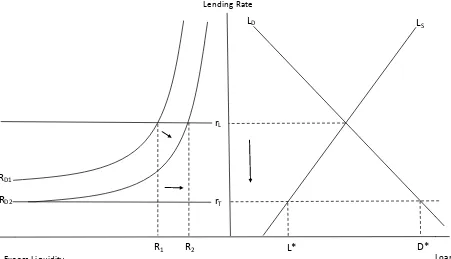
Figure 1 summarizes the core thesis of the bank liquidity trap. The decline in the price of

assets cause the liquidity preference curve to shift fromRD₁toRD2, thereby decreasing the level

(for the given loan rate) of liquidity in the banking system from R₁toR₂. The central bank is now

forced to intervene by pumping excess reserves into the system4. The loan rate declines as the funds rate falls through the liquidity effect. There is no shift in the demand for and supply of

loans. As liquidity is injected the market loan rate falls towards the threshold mark-up rate. At

this point, the rate reaches the non-zero lower bound and the differential between desired loan

demand and actual supply is farthest apart. The desired demand for loans isD*but L*is

supplied by the banking system. The economy has now entered a bank liquidity trap.

3

Open mouth operations would also tend to influence the funds rate in the very short run. Eventually the liquidity effect takes over in longer period observations with which this paper is mainly devoted.

4

6 Figure 1. The Bank Liquidity Trap

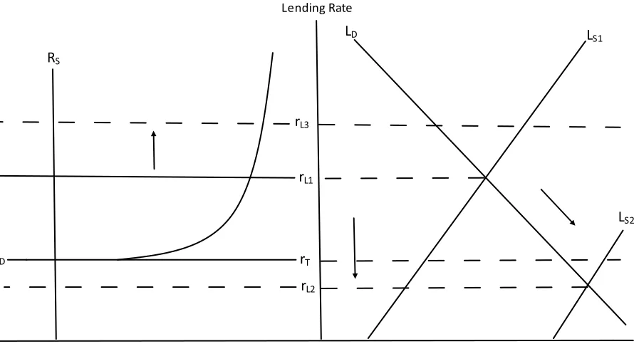
Figure 2 develops the idea further by showing that an outward shift in loan supply

beyondD*cannot occur because it will drive the market rate below the threshold mark-up

lending rate. It implies that the market interest rate rL₂is lower than the risk adjusted marginal

cost of lending; hence banks will be lending to make a loss. This is logically impossible because

banks will not want to drive the market interest rate below marginal cost adjusted for risk of

borrower default. To understand this point further, consider that the Fed has injected enough

liquidity such that the supply of reserves is given by the vertical lineR_S, which intersects the flat

segment of the liquidity preference curve. Once we are in the regime of the BLT, banks will not

extend loans by shifting outwards supply because this causes the market loan rate to fall further

torL₂. Therefore, the BLT can only be characterized by a situation where the non-zero lower

bound lending rate is reached and the desired demand for loans is greater than the actual supply.

On the other hand, excessive monetary tightening can stifle credit demand should it

pressure the market interest rate above equilibrium. This could occur at a market rate such asr_L3

7

in figure 2. If liquidity is drained from the system until it gives rise tor_L3(as shown by equation

5), then the desired supply of loans will now be less than the actual demand for loans. At this

point the economy exited the BLT and entered into a regime in which investment demand is

constrained. Here the parameter would be negative to signal a downward pressure in the lending rate5. It would appear therefore that monetary policy has to walk a balancing act between tightening and easing such that the rater_Lis attained.

Figure 2. In a BLT Banks will not Shift Loan Supply Outwards

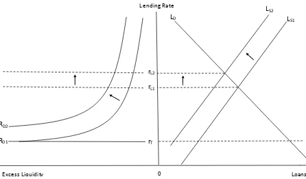
One of the developments after the 2007-08 financial crisis was the payment of interest

rate on excess reserves that banks hold at the Fed. In order to understand how this affects the

model, consider equations 3 and 4. There we see the interest on excess reserves enter both the

liquidity preference equation and the loan supply equation. Given the assumed partial

derivatives, the loan supply function will shift inward and the liquidity preference curve will

5

Oligopolistic banks would tend to quicker to adjust lending rate upward than downward; hence the parameter value will be different in the two regimes. The study of an investment demand constrained regime is beyond the scope of this paper. For an analysis of the investment demand constraint in developing economies, and in an open economy context, see Rodrik and Subramanian (2009).

8

shift outward for an increase inr_E(see figure 3). The effect is that it reduces the intermediation of

loans and increases the level of liquidity. In other words, the policy shifts banks’ preference in favor of excess liquidity. However, the policy would tend to increase the lending rate owing to

its effect on loan supply. In light of the significant decline in the prime lending rate it appears

that the effect of interest on excess reserves has not had this effect to date. The lending rate,

however, could increase as part of an exit strategy if such a strategy involves increasingr_E.

Figure 3. Increase in Interest on Excess Reserves

3. Output and Inflation Dynamics in a BLT

The model presented above needs to be embodied in a macroeconomic framework in

order to analyze how aggregate output and prices behave when the economy is in a BLT. The

framework is based on three equations similar to Khemraj and Proaño (2011). The first equation

is a reserve-loan equation (RL equation) that embeds a reciprocal liquidity preference function,

the second an augmented IS equation, and the third a recursive equation of the Phillips curve.

The IS equation is augmented to take into consideration loan supply of banks. Goodhart and

9

Hofmann (2005) noted that the IS equation should be augmented to include asset prices and

monetary aggregates. This work does not include asset price in the equation because it is not

needed for the problem we seek to address. However, the IS equation can easily be augmented

with borrower net worth so as to analyze how a net worth crash affects output and prices over

time. Including loan supply into the IS equation provides a specification that addresses the problem this paper sets itself addressing.

The RL equation

Assume the lending rate adjusts according to the following specification

1 [ ( , ) ( , , )]

Lt Lt D L FH S L E

r r _  L r N L r r  . However, for the purpose of the analysis at hand we do

not need the shifts in supply and demand for loans. The study will focus only on changes in

interest rate owing to movements along the supply and demand curves. Therefore, the

specification we need for the analysis is given by equation 6. It should be noted that the

framework is general enough for studying output and price dynamics owing to the shift variables

in equations 3 and 4.

1 ( )

Lt Lt D S

r r _  L L (6)

Assume also that the aggregate bank liquidity preference curve takes the shape of a reciprocal

function with the asymptote representing the minimum mark-up interest rater_T. The parameterl

indicates the liquidity effect (0 l 1). For the remainder of this paper assume thatl 1. The stylized facts will show later that this assumption is consistent with an empirical chart of bank

liquidity preference.

l

L T St

r  r R (7)

As noted earlier, in the BLT the supply of loans is the main constraint as the desired demand is

unfulfilled at a specific lending interest rate. Therefore, equation 6 can be rewritten as

1

Lt Lt S

r r _ L . Note that0  1since in the BLT regime interest rate adjustment will be upward given no intervention by the central bank. Substituting equation 6 into 7 and expressing

St

10

1 1

1

( )

St T Lt St

L r r  R

 

 

   (8)

Output dynamics

The augmented IS equation is given by equation 9, while the recursive Phillips curve is

denoted by equation 10. Y_t= aggregate level of output, _t= inflation rate, and Y*= trend output.

r

 = the interest elasticity of output, _L= the loan elasticity of output, = a measurement of

inflation persistence, and = a measurement of the responsiveness of inflation to the output gap. Note that_ris a negative coefficient as the empirical finding of Goodhart and Hofmann (2005) found.

1

( )

t r L t L S

Y  r _  L (9)

*

1 ( )

t t Yt Y

 _   (10)

We now have the basic equations to derive the structural equation which gives the motion of

output over time. The relationship between the federal funds rate and excess liquidity also

follows a reciprocal function, which becomes flat at the zero bound benchmark interest rate. This

relationship will be made obvious in the stylized facts section. Therefore, the expressionr R_F( _S)in

equation 5 can be rewritten as a model given by equation 11.

1

F Z St

r  r R (11)

Substituting equation 11 into equation 5 allows us to rewrite the threshold as

1

(1 )( )

(1 )(1 1/ )

Z St

T

r R mc

r

aN

  



  



 

Note thatr_Z 0as is often noted in the case in a liquidity trap. This is the policy interest rate which the Federal Reserve can increase by policy actions. It is the threshold in equation 11

because the benchmark policy rate has reached its zero bound. This rate must be distinguished

11

benchmark interest rate,r_Tgives the non-zero lower bound lending rate. Substituting forL_Stinto

the IS equation gives

1

1 1

( ) L( ) L

t r Lt t T Lt St

Y  r   r r   R

 



 

     (12)

Note that from the Phillips curve equation we obtaint₁t₂Yt₁assuming stable

parameters. If we substitute this dynamic equation into equation 12 it will give us the following

model that shows how output evolves over time.

1 1 ( 1)

L L

t r t T Lt St

Y  Y  r r   R

 



 

     (13)

Equation 13 suppresses the termr(rLtt₂)which will be reintroduced later when we analyze the inflation dynamics. We now need to substitute equations 11 and 5 into equation 13.

Rearranging and suppressing the expressions ( _L/ )r_Lt1and [ _L/ (1)(1 1/ aN mc)] will

give us the final equation (and taking into consideration the negative_r) that we can use to analyze QE and an interest rate policy in a BLT.

1 1

(1 ) (1 )

(1 )(1 1/ ) (1 )(1 1/ )

L L

t r t Z St

Y Y r R

aN aN

    

  

   

 

 

 

   _  _

  _   _ (14)

Equation 14 allows us to derive and simulate dynamic multipliers for both policies (see

Appendix 1). The interest rate policy would involve increasingrZsince the benchmark policy rate

is close to zero. Quantitative easing policy would involve increasingR_St. The term _r

determines the stability of the equation. It would be necessary to solve for the time path of the

model in order to analyze how the model parameters( ,      _L, _r, , , , , , )a N influence the

relative effectiveness of the two policies. The degree of responsiveness of aggregate output to

loans (measured byL) is critical in determining a positive response in periodt0.  and

affect only the effectiveness of QE, while the percentage of reserves () held in the Fed is

critical for both policies. The speed of lending rate adjustment is crucial for both policies.

12

response int0. One result that might seem counterintuitive is the probability of loan default (

). An increase leads to a bigger response int0. This feature only occurs in a BLT. If the

market rate is above equilibrium we would have the opposite result wherereduces supply of credit. Since the lending rate is at its threshold, the higher risk would signal a higher interest rate

and therefore tend to stimulate intermediation by causing an upward movement along the loan

supply curve (see figure 1).

Price Dynamics

In order to obtain the dynamic price equation, substitute the output solution into the

Phillips curve. This results in the following model in which the term r 2Yt₁is suppressed. For

the purpose of this work assume that the two roots are real, distinct and less than one.

1

1 2

(1 ) (1 )

(1 )(1 1/ ) (1 )(1 1/ )

L L

t t r t rZt RSt

aN aN

      

    

    

 

 

 

    _  _

  _   _ (15)

Using the method of lag operator, the inverse characteristic equation is given as the following.

2

1 2

(1L _r L) (1 L)(1 L); ₁1and₂ 1

This allows us to rewrite Equation 15 as

1 1 1

1 2

(1 ) (1 )

(1 ) (1 )

(1 )(1 1/ ) (1 )(1 1/ )

L L

t L L rZt RSt

aN aN

      

   

   

        

   _  _  _{ }

  _   _

  (16)

4. Stylized Facts

Let us now take a look at the empirical evidence for the existence of a non-zero lower

bound loan interest rate and a zero bound policy rate in a bank liquidity preference framework.

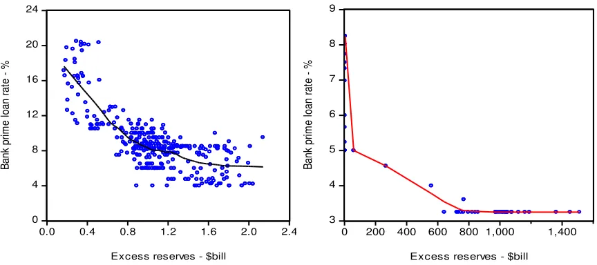
Figure 4 presents a scatter plot of the prime loan interest rate and excess reserves. The plot tends

to confirm a reciprocal shape of the bank liquidity preference curve for the loan rate-excess

reserves space. The reciprocal or the non-zero lower bound rate before the subprime crisis occurs

13

behavior; this time the lower bound threshold declines to approximately 3.25%. The zero bound

benchmark policy rate is an important component of the theoretical model proposed in this work.

Therefore, we must establish this zero bound with a liquidity preference in the space of excess

reserves and the effective federal funds rate. Figure 5 presents the second liquidity preference

curve. Prior to the subprime crisis the lower bound threshold of the effective federal funds rate

was well above zero. However, the threshold fell towards zero, approximately 0.16%, in the

post-crisis period.

Figure 4. Bank liquidity preference vis-à-vis loan rate – monthly data 1980:1–2006:12 (left panel); 2007:1-2012:5 (right panel)

The liquidity preference curves were all extracted from scatter plots using the method of

locally weighted regressions with a smoothing parameter of 0.3 (see Cleveland, 1993; 1979).

Two outliers were removed – those are September 2001 and August 2003. Removing the outliers

does not affect the pre-2007 interest thresholds. Including the outliers makes the threshold rate

more conspicuous. Data for the Loess fit and figure 6 came from the Federal Reserve Economic

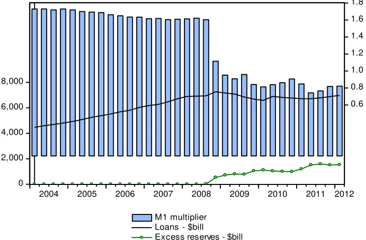
Data (FRED). Figure 6 shows the money multiplier over the period 2004 to 2012: Q1, total loans

and leases and excess reserves. The multiplier has declined significantly as excess reserves

0 4 8 12 16 20 24

0.0 0.4 0.8 1.2 1.6 2.0 2.4 Excess reserves - $bill

B

an

k

pr

im

e

lo

an

r

at

e

-

%

3 4 5 6 7 8 9

0 200 400 600 800 1,000 1,400 Excess reserves - $bill

B

an

k

pr

im

e

lo

an

r

at

e

-

14

expand. As excess reserves rise aggregate loans and leases remain flat, hence being consistent

with the thesis herein that excess reserves and loans are substitutes in a BLT. However, this

substitute relationship would tend to switch to a complement one outside of the regime of a BLT.

Figure 5. Bank liquidity preference vis-à-vis the effective federal funds rate – monthly data 1980:1 – 2006:12 (left panel); 2007:1 to 2012:5 (right panel)

Figure 6. M1 money multiplier (right axis) for quarterly data 2004: Q1 to 2012: Q1

0 4 8 12 16 20

0.0 0.4 0.8 1.2 1.6 2.0 2.4 Excess reserves - $bill

E ff ec tiv e F ed er al F un ds R at e - % 0 1 2 3 4 5 6

0 200 400 600 800 1,000 1,400 Excess reserves - $bil

E ff ec tiv e fe de ra l f un ds r at e - % 0 2,000 4,000 6,000 8,000 0.6 0.8 1.0 1.2 1.4 1.6 1.8

2004 2005 2006 2007 2008 2009 2010 2011 2012

M1 multiplier Loans - $bill

15

5. Model Simulation

The simulations attach numerical values for the derived multipliers in Appendix 1. The

following parameter values are used in the model simulation:_r 0.8, 0.9,_L 0.6, 0.3,

0.2

  , 0.05,₁ 0.9, ₂ 0.4 ,6.52, 6.36and1 1/ aN1. In the case of the latter

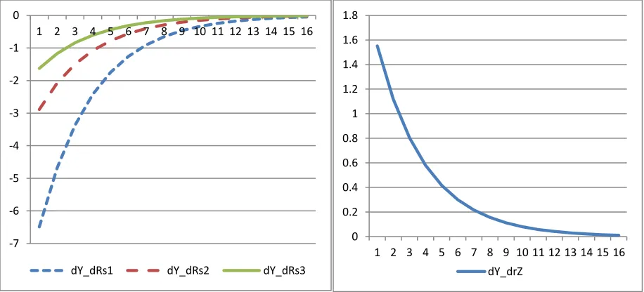
we assume N is so large that the expression representing market power is equal to one. Figure 7

graphs the dynamic multipliers for output change given the change in QE and the policy rate

over sixteen periods after time t = 0. The left panel shows the response of output given an

expansion of monetary easing. Three hypothetical levels of excess reserves are used. The

dynamic multipliers shift inward as the level of reserves increase (RS = 2, RS = 3and RS = 4) at

the binding minimum mark-up lending rate. Overall, the response is negative and tends to move

back to the zero equilibrium. The right panel shows the response of output given a marginal

increase in the zero bound benchmark policy rate. According to the model presented here, the

increase in the interest rate has a positive impact coefficient and eventually dampens towards

equilibrium.

Figure 7. Dynamic response of output to a change in RSand rZ; left panel showsY/RSand right

panel showsY /r_Zfor sixteen future periods

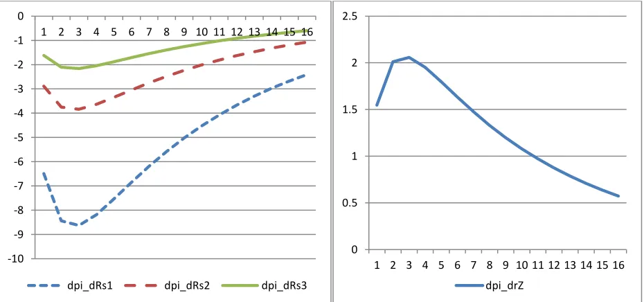
Figure 8 graphs the multipliers showing the response of inflation given a monetary

expansion (left panel) and an increase in the zero bound policy (right panel). The results suggest

-7 -6 -5 -4 -3 -2 -1 0

1 2 3 4 5 6 7 8 9 10 11 12 13 14 15 16

dY_dRs1 dY_dRs2 dY_dRs3

0 0.2 0.4 0.6 0.8 1 1.2 1.4 1.6 1.8

1 2 3 4 5 6 7 8 9 10 11 12 13 14 15 16

16

that monetary easing is deflationary in a BLT regime. The impact multiplier gets less

deflationary as the level of excess reserves increase at the minimum lending rate (RS = 2, RS = 3

and RS = 4). This result is different from other approaches that suggest that the central bank

needs to commit to quantitative easing in order to drive the real interest rate into the negative

territory. However, the liquidity preference of banks means that pursuing QE would be consistent with a falling money multiplier. The derived dynamic multipliers suggest that prices

have to be stimulated through lending (_L) given the responsiveness of inflation to the output gap (). It also suggests that liquidity preference of banks must decline (or the percentage 1 must rise). The output response is positive with an impact multiplier of just over 1.5%.

Subsequent multipliers increase until period 4 and dampen towards equilibrium.

Figure 8. Dynamic response of inflation to a change in RS and rZ: left panel shows/RSand

right panel shows /rZfor sixteen future periods

6. Conclusion

This work proposed a model that integrates excess liquidity and imperfect bank

competition into a dynamic structural macroeconomic framework in order to study how

quantitative easing and an interest rate policy affect output and prices in a liquidity trap, which

-10 -9 -8 -7 -6 -5 -4 -3 -2 -1 0

1 2 3 4 5 6 7 8 9 10 11 12 13 14 15 16

dpi_dRs1 dpi_dRs2 dpi_dRs3

0 0.5 1 1.5 2 2.5

1 2 3 4 5 6 7 8 9 10 11 12 13 14 15 16

17

this paper labels a bank liquidity trap. In this study the non-zero lower bound lending rate was

combined with the conventional zero bound rate through the liquidity preference of banks. The

BLT is precipitated by a shock to bank liquidity preference because of the collapse of financial

asset prices. Subsequent central bank intervention, beyond easing the short-term liquidity freeze,

serves to push the market lending rate towards the risk-adjusted marginal cost of lending, at which point excess reserves and loans are perfect substitutes. Hence, the excess liquidity

phenomenon reflects the idea that the market lending rate is equal to the risk-adjusted marginal

cost of lending. This is different from Murota and Ono (2012) who proposed a model in which the excess bank liquidity signals that households’ marginal utility of cash is greater than that of consumption. The thesis is also different from the explanation given by Keister and McAndrews (2009) who argued that excess liquidity is merely a passive feature of the Fed’s quantitative easing.

The paper proposed the RL equation that is combined with an augmented IS equation and

a traditional Phillips curve. Embedded in the RL equation is a reciprocal function of aggregate

bank liquidity preference, which was then included as a financial friction in a broad

macroeconomic model. This work limited itself to analyzing the implication of bank liquidity

preference for an interest rate policy versus a quantitative easing policy during a bank liquidity

trap in a dynamic setting. However, the framework is general enough that the IS equation can be

expanded to include borrower net worth. The framework can also be extended to study output

and price dynamics in an investment demand constrained regime where the minimum threshold

lending rate is above the equilibrium loanable funds rate. This regime – a subject of future

18

References

Bernanke, Ben and Alan Blinder (1988). “Credit, money and aggregate demand.” American Economic Review, Vol. 78 (2), Papers and Proceedings of the One-Hundredth

Annual Meeting of the American Economic Association, 435-439.

Cleveland, William (1993). Visualizing Data. Summit, NJ: Hobart Press.

Cleveland, William (1979). “Robust locally weighted regression and smoothing scatterplots.”

Journal of the American Statistical Association, Vol. 74: 829-836.

Eggertsson, Gauti (2010). “Liquidity trap.” In Monetary Economics, Durlauf, Steven and Laurence Blume (eds.). New York: Palgrave Macmillan.

Eggertsson, Gauti and Jonathan Ostry (2005). “Does excess liquidity pose a threat in Japan.”

IMF Policy Discussion Paper 05/5, International Monetary Fund.

Enders, Walter (2010). Applied Econometric Time Series, 3ed. Hoboken, NJ: John Wiley and Sons.

Freixas, Xavier and Jean-Charles Rochet (2008). Microeconomics of Banking, 2nd edition. Cambridge, MA: MIT Press.

Goodhart, Charles and Boris Hofmann (2005). “The IS curve and the transmission of monetary policy: is there a puzzle?” Applied Economics, Vol. 37 (1), 29-36.

Gorton, Gary and Andrew Metrick (2010). “Haircuts.” Federal Reserve Bank of St. Louis Review, November/December.

Hamilton, James (1994). Time Series Analysis. Princeton, NJ: Princeton University Press.

Keister, Todd and James McAndrews (2009). “Why are banks holding so many excess reserves?”Current Issues in Economics and Finance, Vol. 15 (8): 1-10.

Khemraj, Tarron (2010). “What does excess bank liquidity say about the loan market in Less Developed Economies?” Oxford Economic Papers, Vol. 62 (1): 86-113.

Khemraj, Tarron and Christian R. Proaño (2011). “Excess bank reserves and monetary policy with a lower-bound lending rate.” Working Paper 04/2011, Department of Economics, New School for Social Research.

Koo, Richard (2009). The Holy Grail of Macroeconomics: Lessons from Japan’s Great

Recession. Hoboken, NJ: John Wiley & Sons.

Krugman, Paul (1998). “It’s baaack! Japan’s slump and the return of the liquidity trap.”

Brookings Papers on Economic Activity, Vol. 29 (2), 137-206.

19

Ogawa, Kazuo (2007). ‘Why Japanese banks held excess reserves: the Japanese experience of the late 1990s.’ Journal of Money, Credit and Banking, Vol. 39 (1): 241-257.

Ono, Yoshiyasu (2011). “The Keynesian multiplier effect reconsidered.” Journal of Money, Credit and Banking, Vol. 43 (4): 787-794.

Rodrik, Dani and Arvind Subramanian (2009). “Why did financial globalization disappoint?”

20

Appendix 1

Derivation of the Minimum Mark-Up Rate

Equation 1A is the representative bank’s profit function (for the ith bank) that is assumed

to be concave in loans to private agents (L_i), deposits (D_i), excess reserves held in special

deposits at the Federal Reserve (RSi), and excess reserves lent out in the interbank federal funds

market (RFi) at the rate of interestrF. Equation 2A is the bank’s balance sheet constraint. 

represents the probability of borrower default; therefore as increases there is a penalty on the profit the bank can make. ( )c Li denotes the costs of monitoring existing loans and making new

loans. This derivation follows the procedure of Freixas and Rochet (2008) and Khemraj (2010).

i (1 ) ( )r L LL i (1 )r RF Fi r R RS( S) Si r D DD( ) i c Li( )

        (1A)

i Fi Si i i

zD R R  L D (2A)

The interest rate earned on special deposits at the fed isr_S. The percent of excess reserves held in

special deposits is and 1percent is loaned out in the funds market. This is obviously a simplification since the profit function does not penalize the bank for having a shortage of

reserves. Omitting the latter feature will not affect the derived threshold lending interest rate. The

level of required reserves is represented byzDiwhere z= required reserve ratio. Except the funds

rate, the key interest rates in the model are written in inverse function forms. r LL( )= loan rate;

( )

D

r D = deposit rate; and r R_S( _S)= interest earned on depositing excess reserves at the fed.

Solving the balance sheet constraint for RFiand substituting into equation 1A gives the

following profit function from which we obtain the first order condition to derive the threshold

equation.

i [(1 ) ( ) (1r LL ) ]r LF i [r RS( S) (1 ) ]r RF Si [ ( )r DD rF(1 )(1 z D)] i c Li( )

            

A Cournot equilibrium is assumed for the purpose of the derivation. In this equilibrium, the ith

21 other words, for the ith bank_{( ,}* *_, *₎

i Si i

L R D solves the profit-maximization problem. The aggregate

quantity of loans, deposits and reserves at the Fed, respectively, demanded by the entire banking

sector are described in equation 3A.

i j

i j

L L L



 



i j

R R R



 



i j

D D D



 



The first-order condition after maximizing the profit function is described by equation

4A. mc= the marginal cost of monitoring existing loans and screening new ones (ormcc L_i( )).

The market demand curve the bank faces is downward sloping, hence the elasticity of demand

denoted by the following expression:a r L rL ( ) /L L. The symbol a is the elasticity of demand

for loans. There is a unique equilibrium in which bank i assumes * *_/

i

L L N, where N denotes

the number of commercial banks that makes up the banking sector. The use of N weighs each bank equally. This is clearly an unrealistic assumption for the purpose of making the mathematics tractable. Nevertheless, the simplification does not change the conclusion of the model. The

expression r LL( )represents the first derivative of the loan rate with respect to L and it is simply

the inverse ofL r( )_L . This allows us to obtainr L_L( ) 1/ L r( )_L . If we substitute this expression

and the elasticity into equation 4 we obtain the equation showing the mark-up over marginal cost

and the funds rate adjusted for the probability of default. This is given by equation 5A.

(1 ) ( ) (1 ) ( ) (1 ) 0

i

L L i F

i d

r L r L L r mc

dL   

 _{        }

(4A)

(1 ) (1 1/ )

(1 )

F L

r mc

r aN 



   

 (5A)

Rearranging equation 5A gives the minimum mark-up rate that we call the threshold

interest rate, r_T(equation 6A). The mark-up is dependent on the inverse of the product of N and

the market elasticity of demand (a) for loans. N=1 describes the case of a monopoly where the

mark-up is highest, while as N  one bank has an infinitesimal share of the market; the equilibrium approaches the purely competitive state in which the mark-up approaches zero. In

22 therefore can be written as ₍ *₎

F

r R with the effect being measured by the derivativer R_F( ), which

is negative thus capturing the trade-off between high liquidity and low interest rate or low

liquidity and high interest rate. This mechanism allows the market interest rate to rise above the threshold at which point the banks’ liquidity preference curve is flat, thus indicating that liquidity effect is zero. Therefore, the threshold loan rate occurs when all funds market liquidity effects

have evaporated. When this occurs the market loan rate is equal to the risk-adjusted marginal

cost of lending. Banks therefore become neutral between hoarding excess reserves and making

loans.

* (1 ) ( )

(1 )(1 1/ )

F T

r R mc

r aN     

  (6A)

Derivation of the Output Multipliers

Equation 14 presented the dynamic structural output equation. Assume an initial value for

output (Y₀) and _r 1. Using a recursive method given the initial value would result in a

solution. Enders (2010) provided a detailed discussion of the solution methods for these types of

dynamic equations. From equation 14 let

1

(1 ) (1 )(1 1/ )

L b aN         and 2 (1 ) (1 )(1 1/ )

L b aN    _       _  _    

A solution to equation 14 is

1 1

1

0 1 2

0 0

( ) ( ) ( )

t t

t i i

t r r Zt i r St i

i i

Y   Y b   r b   R

 



 

 

 





7A allows us to obtain the following dynamic multipliers for i future periods given a change inrZ

23

1( )

i t i r Zt Y b

r  



  

The dynamic multipliers showing the response in output over time for i future periods given a

change inR_Stin the present period are given as follows. The impact multiplier for period i = 0 is

0/ S 2

Y R b

   . Note that the term can easily be 2

S

R eliminated from the expression. However, this

term is kept so as to analyze the impact of quantitative easing when there is a minimum mark-up

lending rate.

2 2( )

i t i r S St Y b R

R  

 

 _{ }



Derivation of the Inflation Multipliers

Equation 15 presented the dynamic structural inflation model. From equations 15 let

3

(1 ) (1 )(1 1/ )

L b aN          and 4 (1 ) (1 )(1 1/ )

L b aN     _       _  _    

We can rewrite equation 16 as





1 1 1

1 2 3 4

(1 ) (1 )

t L L b rZt b RSt

 _{ }  _  _  _(8A)

For the purpose of this work, we will assume that the roots are distinct, real and less than one.

Let us assume that the factor of the inverse characteristic equation can be expressed as follows

2

1 2

(1L _r L) (1 L)(1 L); ₁1and₂ 1

Where

1 2 2 3 3

1 1 1 1

24

1 2 2 3 3

2 2 2 2

(1 L)  1  L L  L ...

Using the method outlined in Hamilton (1994) where  ₁ ₂and applying the method of partial

fractions will result in the following operator:

1 1 2

1 2

1 2 1 2

1

( )

1 L 1 L (1 L)(1 L)

            _  _      

Therefore, we can rewrite equation 8A as

1 1 2 1 1 2 1

1 2 3 1 2 4

1 2 1 2 1 2 1 2

( ) ( )

t b rZt b RSt

L L L L

                          _  _   _  _    

    (9A)

Letc₁   ₁/ ( ₁ ₂); c₂  ₂/ ( ₁ ₂)

This allows for rewriting equation 9A as

2 2 3 3

1 2 3 1 1 2 2 3 1 1 1 2 2 3 2 1 1 2 2 3 3

1 1 2 2 1 3 3

1 2 4 1 1 2 2 4 1 1 1 2 2 4 2 1 1 2 2 4 3

( ) ( ) ( ) ( ) ...

( ) ( ) ( ) ( ) ...

t Zt Zt Zt Zt

St St St Tt

c c b r c c b r c c b r c c b r

c c b R c c b R c c b R c c b r

                              

         (10A)

Or taking the sum gives a solution:

1 1

1 3 1 1 2 2 4 1 1 2 2

0 0

( ) ( )

t t

i i i i

t Zt i St i

i i

b c c r b c c R

       

 

 







From Equation 11A we can obtain the following dynamic multipliers

3( 1 1 2 2)

i i

t i

Zt

b c c

r

_{  }

 _{ }



2 4( 1 1 2 2)

i i

t i

S St

b c c R

R

 _{ } 

 _{  }



The impact multipliers are as follows₀ / r_Z b c₃( ₁c₂)and 2 0/ RSt b c4( 1 c R2) S

 