Munich Personal RePEc Archive
Labor Market Rigidity and Business
Cycle Volatility
Jung, Philip and Kuhn, Moritz
University of Bonn
25 January 2011
Labor Market Rigidity and Business Cycle Volatility
Philip Jung and Moritz Kuhn∗
First Version: July 16, 2009 This Version: January 25, 2011
Abstract
Comparing labor markets of the United States and Germany over the period 1980−2004 uncovers three stylized differences: (1) transition rates from unemployment to employment (UE) were lower by a factor of 5 and inflow rates from employment to unemployment (EU) were lower by a factor of 4 in Germany. (2) The volatility of the UE rate was equal but the EU rate was 2.3 times more volatile in Germany. (3) In Germany EU flows contributed 60−70% to the unemployment volatility while in the U.S. they contributed only 30−40%. We show that these differences can be largely explained by a single factor, namely a lower efficiency in matching unemployed workers to open positions in Germany. Alternative explanations like employment protection, the benefit system, union power, or rigid earnings are likely not the main driving force for the cross-country difference. The lower matching efficiency leads to a substantial prop-agation of shocks. After an adverse shock peak unemployment is reached after 3 quarters in the United States but only after 9 quarters in Germany.
JEL:E02, E24, E32
Keywords: Business Cycle Fluctuations, Labor Market Institutions, Unemployment,
Endoge-nous Separation
∗Jung: Department of Economics, University of Mannheim, L 7, 9, 68131 Mannheim, Germany,
1
Introduction
Compared to the United States the European labor market over the period from 1980−2004 was characterized by high unemployment rates and a sluggish response to shocks. For example, Germany displayed a prolonged period of high unemployment rates in the aftermath of the large oil price shocks, while the U.S. at that time recovered fairly quickly. We document in this paper three important cross-country differences comparing U.S. and German labor market flows: the transition rate from unemployment to employment (UE rate) is lower by a factor of 5 and inflow rates from employment to unemployment (EU rate) are lower by a factor of 4. Second, while (log) UE rates are as volatile, the volatility of the (log) EU rate is 2.3 times larger in Germany compared to the United States. Third, if we decompose the unemployment rate volatility into contributions of EU and UE flows, we find that in Germany the EU flows dominate and account for 60−70% of the unemployment volatility, while in the U.S. they account for only 30−40%.1
In this paper we propose an explanation for all three differences that is based on a common source, a lower efficiency in matching unemployed workers to open positions in Germany. We show that the empirical cross country comparison offers identification restrictions that can be used to disentangle our explanation from prominent alternatives that have been proposed in the literature to rationalize either the lower average transition rates across country or the differences in the volatilities. To our knowledge our paper is the first to simultaneously look at salient labor market features across the two countries both in the mean rates and the business cycle dynamics and to link them to structural differences in a common framework.
For this purpose, we develop a simple labor market search and matching model with endogenous separations. We adapt the model to study business cycles in a similar fashion as den Haan, Ramey, and Watson (2000) and Ramey (2008). We derive simple closed form solutions for the second moments, so that we can analytically characterize the implications of institutional changes on the reaction to business cycle shocks. To study the different explanations in a unified framework we allow for worker and firm specific human capital accumulation, persistent idiosyncratic shocks as in Costain, Jimeno, and Thomas (2010) and tenure-dependent firing taxes.
A lower efficiency in the matching process in Germany relative to the U.S. leads to a decline in the frequency of UE transitions due to an effective increase in the cost of creating an open position. Simultaneously the average match surplus increases due to a deterioration of the outside opportunities of employed workers induced by the longer search duration. The increase in the average match surplus makes is less likely that negative idiosyncratic shocks destroy a match, so the frequency of transitions from employment into unemployment declines. However, differences in matching efficiency not only influence average transition rates. The increase in the average surplus makes German workers more sensitive to business cycle shocks.
1For the U.S. Hall (2005) and Shimer (2007) emphasizes the importance of the UE flows in understanding labor
Consider a German worker at the beginning of a boom. In case she separates, she has to search longer to find a new match compared to a U.S. worker due to the lower average UE rate. She would miss a larger fraction of the most profitable time of being employed. This will make her more reluctant to separate. Similarly, at the onset of a recession the German worker is more willing to separate because she will only miss the least profitable time of being employed while searching for a job. As a result, the German EU rate decreases more strongly in booms and increases more strongly in recessions, i.e. it is more volatile. The EU rate volatility is driven by the absolute change in the surplus of a match while the UE rate volatility is driven by the relative change of the surplus to its long run average. This remains largely unaffected due to the simultaneous increase in the average surplus and the increase in the sensitivity of the surplus to shocks. Hence, the contribution of the EU rate in the unemployment volatility increases. A lower matching efficiency can therefore explain both the difference in average transition rates as well as the differences in the second moments between the two countries.
We consider four alternative explanations and show that these cannot explain all three cross-country differences at the same time. First, explaining the lower UE rates in Germany by a more benevolent unemployment insurance system, larger firing taxes and/or an increase in micro-economic turbulence Ljungqvist and Sargent (2008); Wasmer (2006) will lower the average match surplus and increase the outflow volatility by more than the inflow volatility, inconsistent with our empirical facts. The second alternative, we consider, is a stronger bargaining position of the worker in Germany possibly induced by the employment protection legislation Blanchard and Portugal (2001). This can explain the lower UE rate but not the larger EU rate volatility. We show that at the Hosios condition Hosios (1990) both the average surplus and, as a consequence, the EU rate volatility are minimized. A deviation from the Hosios condition is quantitatively too small to jointly account for the lower UE rates and the large differences in the volatilities we observe in the data. Third, we consider differences in firing taxes between low and high tenured worker Bentolila, Cahuc, Dolado, and Barbanchon (2010); Costain, Jimeno, and Thomas (2010). Yet, these lead to an increase in the UE rate volatility and to inconsistencies in the tenure pattern of the transition rates which we document empirically. Fourth, explanations based on rigidities in the wage setting process Shimer (2010); Elsby and Michaels (2010) affect, in models with endogenous destruction, the EU rate and the UE rate volatility symmetrically, leaving the contribution of inflows to the unemployment volatility unaffected, again inconsistent with the empirical facts.
United States.
The paper is related to the growing body of literature studying the European ins and outs of unemployment Petrongolo and Pissarides (2008); Pissarides (2009) based on micro-data and Elsby, Hobijn, and Sahin (2010) using aggregate OECD data. We provide a detailed account on the ”ins and outs” for Germany using a large micro data set on employment histories.2 We extend the unemployment volatility decomposition developed in Fujita and Ramey (2005) and Petrongolo and Pissarides (2008) to a three state, six transition rate decomposition to particularly control for flows in and out of inactivity. We provide new evidence on the transition rates by tenure to shed light on the impact of differential firing taxes and the skill accumulation process. Finally we give a complete account on the earning dynamics in Germany, controlling for selection effects using various methods proposed in Bils (1985), Solon, Barsky, and Parker (1994) and Haefke, Sonntag, and van Rens (2007) to empirically assess the possible importance of wage rigidities across countries. The remainder of the paper is organized as follows: Section 2 documents labor market facts for Germany, section 3 develops the model, section 4 characterizes the results, extensions are in section 5, and section 6 concludes.
2
Data
2.1 Data description
Our dataset is the IAB3 employment panel that comprises a 2% representative sample taken from
the German social security and unemployment records for the period 1980−2004. The sample contains employees that are covered by the compulsory German social security system, and excludes self-employed and civil servants (’Beamte’). It covers about 80% of Germany’s labor force. Since the East German labor market was subject to additional regulations and restructuring after the reunification, we exclude all persons with employment spells in East Germany from our sample.4 For each worker in the sample we observe the entire employment history (social security status) on a daily basis. We choose as our basic period length one month and construct monthly employment
2Burda and Wyplosz (1994) summarize evidence on average transition rates for Europe. There are two other
studies on worker flows using the IAB in Germany that show a limited amount of overlap with our results. Bachmann (2005) uses a slightly different concept to measure worker flows. He measures worker flows on a monthly frequency but focuses for the dynamics at an annual frequency. However, his results regarding average transition rates are consistent with our findings. Very recently Gartner, Merkl, and Rothe (2009) also report some basic facts but use different definitions for labor market states, for example they do not control for inactivity, and work with a quarterly aggregation so that their results are not comparable to our findings.
3This study uses the factually anonymous BA-Employment Panel (Years 1975−2004). Data access was provided
via a Scientific Use File supplied by the Research Data Centre (FDZ) of the German Federal Employment Agency (BA) at the Institute for Employment Research (IAB).
4We do a first step sample selection where we remove very few individuals with missing observations. Details on
histories from the daily data.5 We account explicitly for periods of inactivity and transitions out of the labor force, e.g. (early) retirement or maternity leave.
Aggregate data for Germany are from the German statistical office (’Statistische Bundesamt’). The official unemployment rate is from the German Employment Agency (’Bundesagentur f¨ur Arbeit’).6 The data for the U.S. is from the BLS for the aggregate time series and from Shimer (2007) for the labor market transition rates. The numbers on employer-to-employer transitions are from Fallick and Fleischman (2004). In the decomposition analysis of the unemployment volatility we use in addition data from Fujita and Ramey (2009).
2.2 Labor market flows
Following the work of Shimer (2005) for the United States and Petrongolo and Pissarides (2008) for several European countries this section provides a comprehensive analysis of the ‘ins and outs’ of unemployment for Germany and compares the results to existing evidence for the United States.7 Table 1 summarizes our findings and presents a cross-country comparison along three dimensions: aggregate business cycle fluctuations, mean labor market transition rates, and volatilities of the transition rates.8 Two facts are striking, while the aggregate business cycle fluctuations look very much alike (see left part of the table), the transition rates in the right part of the table uncover a labor market that is substantially different both in mean rates and in volatilities (see right part of the table).
More specifically, measures of aggregate economic activity GDP, labor productivity, and earnings have similar volatilities in both countries. The aggregate measures of the labor market are slightly more volatile in Germany compared to the U.S.. The unemployment rate is 1.2 times as volatile and vacancies9 are 1.6 times as volatile. Correlations with GDP have the same sign and similar magnitudes across the two countries. Additionally the Beveridge curve, the correlation between unemployment rates and vacancies, is strongly negative in Germany (correlation −0.85) and the U.S. (correlation−0.91). Altogether, the picture that emerges on an aggregate level is fairly similar. This changes once we look at labor market transition rates and volatilities in the right part of the table. We find average rates that are substantially lower in Germany. The EU rate is lower by a factor of 4 and the EE and EN rates differ by a factor of approximately 3. The UE rate is also
5In the appendix we describe in detail how we construct the employment histories and labor market states.
Bachmann (2005) studies an earlier version of our dataset covering the period 1975−2001 and applies a different approach to measure labor market transition rates. His results account for all transitions within a month but are virtually unchanged compared to our findings.
6Further details especially on the adjustment for the German reunification can be found in the appendix.
7The data discussed here refers to all workers and an online appendix to this paper provides an extended analysis
where we separate worker flows based on sex and education.
8We do not report NU and NE transition rates because we do not observe the universe of all non-employed so that
transition rates can not be computed. The online appendix reports the correlation and volatilities for these flows.
9We only have notified open positions at the job centers that do not constitute the whole universe of open positions.
Table 1: GDP, unemployment rates, and transition rates over the business cycle
Statistic mean std corr Transition rate
mean std corr
Germany
GDP 2.4 1 EU 0.5 15.1 -0.81
U.S. 2.6 1 2.0 6.5 -0.72
Germany
Productivity 1.6 0.77 UE 6.2 10.4 0.40
U.S. 1.4 0.44 30.7 11.2 0.82
Germany
Earnings 1.7 0.84 EE 0.9 15.6 0.65
U.S. 1.8 0.42 2.6 6.3 0.65
Germany
Vacancies 33.4 0.82 EN 1.0 6.2 0.53
U.S. 20.4 0.85 2.7 4.6 0.44
Germany
Urate 8.4 18.1 -0.76 UN 4.9 10.3 0.45
U.S. 6.3 15.0 -0.89 26.6 9.1 0.73
Notes: Standard deviations (STD) are given as percentage deviations from an HP-filtered trend (λ= 100000) of the rates (in logs). Correlations (CORR) give the correlation coefficient with GDP. Our productivity measure is GDP per employed. Source: Authors’ own calculations based on IAB data.
substantially lower and differs by a factor of 5.10 A reverse picture arises for the volatilities. While
the UE rates in both countries are still equally volatile, the German EU rate turns out to be 2.3 times more volatile than the U.S. rate.11 Figure 1(a) visualizes the close connection of the cyclical component of the EU rate and the unemployment rate in Germany while the link is present but not as close in the U.S. (Figure 1(b)).
(a) Germany
1980 1985 1990 1995 2000 2005 −0.6
−0.5 −0.4 −0.3 −0.2 −0.1 0 0.1 0.2 0.3
(b) United States
1980 1985 1990 1995 2000 2005 −0.3
−0.2 −0.1 0 0.1 0.2 0.3 0.4
Figure 1: Cyclical component of EU rate and unemployment rate
Notes: The figure shows the cyclical component of the EU rate and the official unemployment rate based on an HP-filter (λ= 100000). The red solid line is the EU rate and the blue dashed line is the unemployment rate.
The exit rate (EU + EN) tends towards acyclicality both in Germany (correlation −0.47) and the
10These lower rates can be observed throughout the sample period and are not an artifact of the developments
in the nineties. In 1980, the average UE rate in Germany is 10.9% declining over time to 4.7% in the mid-nineties (1995). During the same time period the EU rate increased from 0.4% to 0.5%.
11Given that we study the interaction of long-run means and cyclical volatilities and the long lasting consequences
[image:7.612.130.475.335.499.2]U.S. (correlation −0.24). This is due to countercyclical EU rates and procyclical EN rates. Only for Germany, we have EE flows for the whole sample period. If we add these to the total separation rate (EU + EN + EE), the correlation turns positive (correlation 0.46) as a consequence of the procyclical EE flows. These results suggest that EN flows are rather different to EU flows and seem to have more in common with EE flows than with EU flows. Support for this view comes from Nagypal (2005). She shows that for the U.S. many EN flows are reverted one month later suggesting possibly the move to a new employer with an intervening month of inactivity.
2.3 Unemployment decomposition
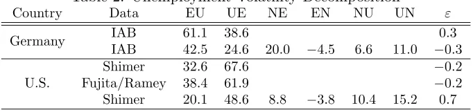
[image:8.612.136.477.300.381.2]To address the importance of in- and outflows in explaining unemployment volatility, we use the methodology proposed in Fujita and Ramey (2009) but develop also an extended decomposition with three states and six transition rates to control for flows into inactivity. Details on the volatility decomposition of Fujita and Ramey (2009) and our extension can be found in Appendix A.1.12 Table 2 summarizes our finding based on the two state and three state decomposition where the numbers present the share in unemployment volatility attributed to the respective rates.
Table 2: Unemployment Volatility Decomposition
Country Data EU UE NE EN NU UN ε
Germany IAB 61.1 38.6 0.3
IAB 42.5 24.6 20.0 −4.5 6.6 11.0 −0.3
U.S.
Shimer 32.6 67.6 −0.2
Fujita/Ramey 38.4 61.9 −0.2 Shimer 20.1 48.6 8.8 −3.8 10.4 15.2 0.7
Notes: Data is HP-filtered (λ= 100,000) for the period 1980q1−2004q4. For Germany the transition rates are for all workers. The U.S. data is obtained from Shimer (2007) and Fujita and Ramey (2009). Contribution shares are given as percentage numbers. Source: Authors’ own calculations based on IAB data.
Based on a two state decomposition the contribution of EU rates account for more than 60% of the volatility in unemployment while in the U.S. it accounts for 30−40%. The three state decomposition indicates that German EU rates contribute about twice as much to the unemployment volatility as the UE rates, while in the U.S. the opposite is the case. EU and UE rates taken together account in both countries for around 2/3 of the unemployment volatility possibly justifying the focus on a
12Petrongolo and Pissarides (2008) analyze the contribution of job in- and outflow rates to the fluctuations in
two-state decomposition.
Our empirical findings show that the German labor market is characterized by substantially lower average transitions rates compared to the U.S. Despite a similar UE rate volatility the German EU rate volatility though is substantially larger. In reaction to shocks the German labor market relies more heavily on adjusting the inflow rate while the U.S. labor market relies more on the outflow rate.
3
Model
To understand the differential labor markets in the two countries we develop an extended version of a Mortensen-Pissarides-style search and matching model. In the general version of the model we allow for a generic idiosyncratic state process which we will later attach specific forms in order to model tenure on the job, individual or match specific skills.
There is a continuum of workers with measure one. Workers and firms are risk neutral. Workers can be either employed or unemployed denoted by ˜e ∈ {e, u}. The aggregate technology state A
is random and follows a Markov process. Additionally, there is an idiosyncratic state attached to each worker denoted by x∈X. This state also follows a Markov process. We allow this process to
depend on the labor market transition from the current labor market state ˜eto next period’s state ˜
e′, for example to model the loss of firm specific human capital after an EU transition (turbulence). This means the model has different conditional distributions over tomorrow’s idiosyncratic state depending on current and future employment status. We denote these distributions by pee(x′|x), peu(x′|x), pue(x′|x), and puu(x′|x) depending on wether the agent stays employed, moves into unemployment, out of unemployment or stays unemployed, respectively.
The measure of unemployed workers in the different idiosyncratic states is denoted byu(x) and for employed workers byl(x). The joint distribution over employment states ˜eand idiosyncratic states
x isλ:{e, u} ×X→[0,1] where Λ denotes the set of possible joint distributions.
Time is discrete. Workers who are currently in a match bargain jointly and efficiently over the wage and the separation decision for the next period. If the bargaining is successful, they produce output according to the production technology Ag(x) where the aggregate technology A evolves exogenously and common to all matches, and g(x) summarizes the individual productivity for a worker of type x. At the end of the period, the firm receives an idiosyncratic cost shock ε. We assume that ε is i.i.d. across firms and over time and logistically distributed with mean zero and variance π32ψ2ε. The assumption of a logistic distribution allows us to obtain closed form solutions and is done for convenience. The firm has to pay the costs ǫ only if it wishes to continue the production process. The costs are sunk after the period and will not affect any future decision. At the bargaining stage the firm and the worker agree upon a threshold value ¯ǫ for the continuation costsε.
the firm has to pay a state dependent firing tax τ(x) to the government and the worker becomes unemployed. The transition probability for the individual state in this case is peu(x′|x).13 If the costs ǫ are smaller than the cut-off value ¯ǫ, then they the firm pays the continuation costs and continues the match. In this case, the worker transits to a new idiosyncratic state with probability
pee(x′|x). This structure of the optimal decision allows us to cast the separation decision solely in terms of cut-off values.14
An unemployed worker searches for a job and is matched in a matching market governed by a stan-dard Cobb-Douglas matching function. Search is random so unemployed workers receive job offers from firms with probabilityπue. Together with the offer comes a realized idiosyncratic productivity component. The probability distribution for the idiosyncratic state ispue(x′|x). In case the worker does not receive an offer, a new idiosyncratic state is drawn according to puu(x′|x). While unem-ployed, a worker has a utility flow ˜b(A, x) which might depend on the current idiosyncratic state but also on the aggregate state. We include the dependence on the aggregate and idiosyncratic states to capture in a simple way the effects of wage rigidity. Specifically, we use ˜b(A, x) = exp(ϕ(x) log(A))b. This functional form includes the different cases studied in the literature. Using ϕ= 1, we mimic very flexible wages, usingϕ= 0, we have our benchmark case used in Shimer (2005) and Hagedorn and Manovskii (2008), and usingϕ <0, we can mimic a stronger form of wage rigidity inducing a countercyclical element to the surplus that will amplify shocks.15
Consider a worker-firm pair at the beginning of the period. The firm discounts the future, as does the worker, with a constant discount factor β. For given wages w :R×X×Λ → R+ and cut-off
13Note thatτ(x) is expressed as a firing tax, or a reorganization cost and does not include severance payments.
In our framework, severance payments are efficiently bargained away and would have no effect on the equilibrium outcomes. The government transfers all income lump sum back to the worker, so under risk-neutrality, there is no need to formally specify governmental behavior.
14Technically, the cut-off value represents a quantile of the cost shock distribution and the cost shockεitself will
not appear explicitly in any further expression.
15We allow for a possible type dependence on the idiosyncratic state to include the case were newly employed
strategies ¯ǫ:R×X×Λ→R+ the firm’s surplus and the probabilityπeu are given by16
J(A, x, λ) = Ag(x)−w(A, x, λ)
+
Z ¯ǫ
−∞ βE " X x′
pee(x′|x)J(A′, x′, λ′)
#
−ε
df(ε)−
Z ∞
¯
ǫ
τ(x)df(ε) (1)
πeu(A, x, λ) = 1−P rob(ε <¯ǫ) =
1 + exp
¯
ǫ(A, x, λ)
ψε
−1
.
The value functions for employed workers Ve : R+×X×Λ → R and unemployed workers Vu :
R+×X×Λ→Rare given by
Ve(A, x, λ) = w(A, x, λ) + (1−πeu(A, x, λ))βE
"
X
x′
pee(x′|x)Ve(A′, x′, λ′)
#
+πeu(A, x, λ)βE
" X
x′
peu(x′|x)Vu(A′, x′, λ′)
#
(2)
Vu(A, x, λ) = bexp(ϕ(x) log(A)) + (1−πue(A, λ))βE
"
X
x′′
puu(x′′|x)Vu(A′, x′′, λ′)
#
+πue(A, λ)βE
"
X
x′
pue(x′|x)Ve(A′, x′, λ′)
#
. (3)
We denote the worker’s surplus by ∆(A, x, λ) =Ve(A, x, λ)−Vu(A, x, λ) and the match surplus as S(A, x, λ) =J(A, x, λ) +Ve(A, x, λ)−Vu(A, x, λ).
New matches are formed by a standard Cobb-Douglas matching technology that links searching workers to vacancies. The measure of unemployed workers is denoted by u, the vacancies posted are denoted by v, and the resulting matches by m.
m = κv1−̺u̺
u = X x∈X
u(x).
16Solving the conditional expectation forπ
eu(A, x) the firm’s profit is
J(A, x, λ) =Ag(x)−w(A, x, λ) + (1−πeu(A, x, λ))βE
" X
x′
pee(x′|x)J(A′, x′, λ′)
#
−πeu(A, x, λ)τ(x) + Ψ(A, x, λ).
Evaluating the integrals under the distributional assumptions yields the given functional form. The option value Ψ follow directly from the assumption of a logistically distributed cost shock and captures the value of having a choice to continue the match and is always positive
Ψ(A, x) = −ψε
(1−πeu(A, x, λ)) log(1−πeu(A, x, λ)) +πeu(A, x, λ) log(πeu(A, x, λ))
The matching efficiency κ measures how effectively unemployed workers are matched to open
positions. Examples for factors that can influence the matching efficiency are the willingness of workers to move for a new job, skill mismatch, or bureaucracy in employment agencies. Labor market tightness is defined as usual as the ratio of vacancies to searching workers θ := vu. The probability that a searching worker will meet a firm is
πue(A, λ) = m
u =κθ
1−̺
and the probability that a firm posting a vacancy will meet some worker is given by
πve= m
v =κθ
−̺.
To determine the number of vacancies posted, we impose a standard free entry condition
κ=πve
X
x∈X
u(x)
u βE
"
X
x′
J(A′, x′, λ′)pue(x′|x)
#
.
The probability of meeting a specific worker with characteristicsxisu(ux). We assume Nash bargain-ing jointly over wages and cut-off values. The outcome of the bargainbargain-ing process is characterized by
{w,ω¯}= arg max
w,ω¯ µlog (∆(A, x, λ)) + (1−µ) log (J(A, x, λ))
whereµ denotes the bargaining power of the worker. First-order conditions deliver
¯
ω(A, x, λ) = βE
" X
x′
pee(x′|x)(J(A′, x′, λ′)
+Ve(A′, x′, λ′))−
X
x′
peu(x′|x)Vu(A′, x′, λ′)
#
+τ(x)
µ
1−µ =
∆(A, x, λ)
J(A, x, λ).
Technology evolves exogenously according to
A= exp(a) a′ =ρa+η′
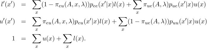
status whose laws of motion are given by:
l′(x′) = X x
(1−πeu(A, x, λ))pee(x′|x)l(x) +
X
x
πue(A, λ)pue(x′|x)u(x)
u′(x′) = X x
πeu(A, x, λ)peu(x′|x)l(x) +
X
x
(1−πue(A, λ))puu(x′|x)u(x)
1 = X
x
u(x) +X x
l(x).
4
Baseline Specification and Results
This section explains why the cross-country differences we document empirically can be explained by differences in the matching efficiency. In our baseline specification presented in this section we specialize to the homogeneous worker case abstracting from idiosyncratic shocks, i.e. we setx= 1, so all policy rules are functions of the aggregate state only.17 We first characterize the working of
the model and explain why it accounts for the cross-country differences in the first and the second moments jointly. To do so, we provide an analytic link between the structural parameters of the model capturing institutional differences across countries and these moments. Finally, we offer a quantitative exploration.
[image:13.612.132.484.52.139.2]4.1 Basic Mechanism
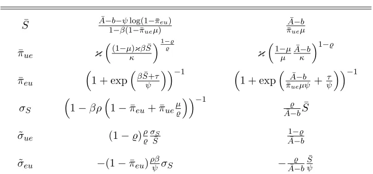
Table 3 shows the steady state of the model and gives an analytical characterization of the volatilities based on a first-order approximation, whereσy captures the deviation of a variableyfrom its steady state value ¯y when the productivity state isa, i.e. y−y¯=σyaand ˜σy = σy¯y denotes the percentage deviation. The absolute value of ˜σy coincides with the log standard deviations relative to the standard deviation of productivity. We also report some simple approximations to the resulting expressions to gain intuition.
As Table 3 shows the EU rate volatility (|˜σeu|) is linear in the surplus reaction σS scaled by the standard deviationψof the continuation-cost. Intuitively, less dispersed cost shocks lead to a larger fraction of firms living around the cut-off value ¯ǫ. As a consequence, a change in the surplus after a business cycle shock will lead to more firms that draw cost shocks below the cut-off value and decide to dissolve. At the aggregate level this implies an increase in the EU rate after a negative business cycle shock making EU rates countercyclical.18
Unlike the EU rate volatility theUE rate volatility (|˜σue|) is linear in the relative surplus volatility σS
S . This makes the UE rate volatility a direct function of the outside optionb(see approximation), a
17In the absence of idiosyncratic shocks the model is block-recursive in the sense of Menzio and Shi (2009) so the
employment measure does not enter the policy functions.
18This is the standard logic of generating countercyclical EU rates and applies as well to models using log-normal
Table 3: Analytic Expressions for the First and Second Moments
Exact Approximation
¯
S A¯−b−ψlog(1−π¯eu)
1−β(1−π¯ueµ)
¯
A−b
¯
πueµ
¯
πue κ
(1−µ)κβS¯
κ
1−̺̺
κ1−µ
µ
¯
A−b κ
1−̺
¯
πeu
1 + expβS¯ψ+τ−1 1 + expπ¯A¯−b
ueµψ + τ ψ
−1
σS
1−βρ1−π¯eu+ ¯πueµ̺
−1
̺
¯
A−bS¯
˜
σue (1−̺)ρ̺σS¯S A1¯−−̺b
˜
σeu −(1−¯πeu)ρβψσS −A¯̺−b
¯
S ψ
Notes: Analytic exact expressions for steady states are in the first column. Approximations usingβρ≈1 andπEU ≈0
are given in the second column.
fact that has been discussed in the recent literature Shimer (2005); Hagedorn and Manovskii (2008). As a consequence, our calibration will require an outside option b that is close to productivity to match the UE rate volatility, but this is not decisive for our argument as we show in section 5. The presence of endogenous destruction has no first order effect on the UE rate volatility. Separations are efficiently bargained and reflect a choice of the match, so their impact is of second order on the dynamics of the relative change in the surplus. However, endogenous destruction affects the model’s unemployment rate volatility.
|˜σu| =
|σeu(1−u¯)−σueu¯| ¯
up
1−(1−¯πue−π¯eu)2
s
1 +ρ(1−π¯ue−π¯eu) 1−ρ(1−π¯ue−π¯eu) ≈ (|˜σeu|+|˜σue|)(1−u¯)
The contribution of the EU rate to the unemployment volatility is essentially driven by the ratio |˜σeu|to |˜σue|.19 Using the approximation from table 3, we see that the contribution of the EU rate to the unemployment volatility is proportional to the average surplus
|˜σeu| |˜σue|
= ̺
1−̺
¯
S ψ
and to explain a higher contribution of EU transitions to the volatility of the unemployment in
19The formula shows that a cross-country comparison should be based on the volatility of the percentage deviation
Germany we directly see that the average surplus has to be larger.
The EU rate volatility |˜σeu|is an increasing function of the average match surplus and is inversely related to the average UE rate (cp. approximation in table 3). The intuition for the inverse relationship has its seeds in the reemployment prospects of workers after separation. This can be seen by looking at the recursive formula of the surplus obtained from equations (1), (2) and (3), where we set ψǫlog(1−πeu)≈0 for simplicity
S≈A−b+βES′−πU EµES′.
We see that the current surplus is the discounted surplus of the current match A−b+βE[S′] net
of the outside opportunity πU EµE[S′] in an alternative match of the worker.20
Consider now how a positive business cycle shock affects these two values. The surplus of the current match increases making it less likely that an idiosyncratic shocks hitting the match will lead to a separation. As a result, the EU rate falls making it countercyclical. At the same time, the increase in the surplus of the current match is dampened by the reaction of the outside opportunity of the worker which enters negatively into the total surplus and will therefore lower the reaction
σS. In a boom the outside opportunity will increase because the prospects of finding a job quickly increase and the expected surplus of an alternative match also rises.
The cross-country differences in the outside opportunity explains the differences in the reaction to shocks. Take Germany that has a lower average UE rate. At the onset of a boom, the opportunity costs of separating for the German worker are higher because she misses particularly productive times. On average the German worker searches for a new job for roughly a year and the worker has missed the most profitable times of being employed. This makes her more reluctant to separate in reaction to the shock. The U.S. worker instead needs to search on average only three months and is still able to benefit from the booming conditions by quickly accepting a new job offer. As a consequence the increase in the outside opportunity in the U.S. is stronger at the beginning of a boom compared to Germany. This dampens the reaction of the surplus and ultimately lowers the EU rate volatility.21
20We use the termoutside opportunity because it captures the expected value of an alternative match in case of
separation.
21A corresponding argument shows that at the beginning of a recession the German worker will be more willing to
4.2 Institutional Factors
[image:16.612.112.503.195.366.2]What institutional factors can explain the observed differences in labor market outcomes between the U.S. and Germany? Our intuition developed so far has focused on the transmission from mean transition rates to volatilities, which are both endogenous objects. We now provide the link to the underlying structural parameters. Table 4 reports the analytic elasticities of the average rates and the volatilities with respect to a change in the underlying parameter. They can be used to sign the impact of each of the structural parameters on the four endogenous dimensions considered in this paper.22
Table 4: Analytic approximations of steady state elasticities
p Parameter πp ue dπue dp p πeu dπeu dp p
|σ˜eu| d|σ˜eu|
dp
p
˜
σue dσ˜ue
dp
κ Matching
Effi-ciency
̺
1−̺
̺
1−̺
¯
S
ψ −
̺
1−̺ 0
µ Bargaining Power
−11−−µ̺ −1µ−−µ̺Sψ¯ µ1−−µ̺ 0
b Outside Option −(1A¯−−̺b)b µψ̺bπ¯
ue (1−̺) b
¯
A−b
b
¯
A−b
τ Firing Tax −(1−̺)τπ¯eu
¯
A−b −(1− ̺¯πeu µπ¯ue)
τ
ψ (1−̺) τπ¯eu
¯
A−b
τπ¯eu
¯
A−b
ψ Shock Variance −Ψ(1¯A¯−−b̺) τ+ ¯ψS +ψµΨ¯¯π̺
ue −
1−Ψ(1¯A¯−−b̺) A¯Ψ¯−b
Notes: Approximation to the steady state elasticities. ¯Ψ is the steady state value of the option value from the separation decision. The approximation is based onβρ≃1.
The upper part of table 3 shows that there are essentially three options to generate lower average UE rates in Germany: First, a lower efficiency of the matching function κ in Germany and an
associated increase in the effective cost per unit of vacancies posted. The parameter captures in a reduced form sense frictions in the entry process like for example skill, occupational, or regional mismatch. A decline lowers the average UE rate, increases the surplus of the match, and lowers the average EU rate. The UE rate volatility remains unchanged because the increase in the surplus is accompanied by an increase in the effective cost to post a vacancy, keeping the percentage change in the surplus largely unaffected. The EU rate volatility increases by the same factor as the average UE rate declines (cp. table 4, first row) matching therefore all of our stylized facts qualitatively. Second,higher benefits b as argued for in Ljungqvist and Sargent (2008) lowers the surplus of the match, lowers profits, and the average UE rate. The lower surplus would lead to a counterfactual
22To obtain the elasticities we make use of the fact that both the average rates and the volatilities are simple
increase in the average EU rate, so this option has to rely on additional firing taxes τ to jointly explain the mean rate differences across countries. Still, the mechanism will be inconsistent with the second moments of the data. The third row in table 4 shows that the reaction of the EU rate volatility (|˜σeu|) is always lower by a factor 1−̺compared to the reaction of the UE rate volatility (|˜σue|). Therefore a decline in the surplus will unambiguously decrease the contribution of inflows relative to outflows in the unemployment volatility and will be inconsistent with the empirical evidence. A similar argument can be made for higher firing taxes (cp. table 4, fourth row). Third, a higher bargaining power of the worker µ in Germany lowers the share of the surplus accruing to the firm. This lowers the incentives to create jobs, and thereby lowers the average UE rate. This mechanism is used for example in Blanchard and Portugal (2001) who argue that the employment protection legislation implicitly increases the threat point of the worker, and therefore effectively raises the bargaining power. The effect of a higher bargaining power on the average surplus is ambiguous and depends on the distance to the Hosios point of efficiency (cp. table 4, second row). Two counteracting forces are at work: a higher bargaining power lowers the UE rate which tends to increase the average surplus as explained above. But at the same time the outside opportunity of the worker raises relative to the current match which tends to lower the average surplus. Exactly at the Hosios condition the surplus is minimized23 and the bargaining power of the workerµis equal to the matching elasticity ̺. To see this, we implicitly differentiate the steady state surplus with respect to the bargaining power
∂S ∂µ =
µ−̺
1−µ
βS¯π¯ue
̺1−β+βπ¯eu+µ̺π¯eu
It can be immediately verified that the surplus has its minimum at the Hosios condition.24 In-tuitively, the benchmark scenario of a perfectly competitive market without search and matching friction would compete the surplus to zero, making all workers employed, and force wages to be equal to productivity. The matching frictions impose a deviation from this benchmark leading to a positive surplus. The social planner minimizes this deviation by putting the economy at the Hosios condition given all other parameters. As a result, the EU rate volatility is also minimized. Due to the sign switch in the elasticity of |˜σeu| at the Hosios condition (cp. table 4, second row) a cross-country change in the bargaining power can therefore increase or decrease the EU rate volatility depending on the initial conditions. To the extend that the change in the bargaining power is large enough the channel works similarly to a change in the match efficiency. It lowers the gains from posting a vacancy and simultaneously increase the surplus of the match. However, the outside opportunity of the worker is directly affected which tends to dampen the EU rate volatility
23Despite our endogenous destruction mechanism, it is straightforward to show that the Hosios condition still holds
in our framework, conditional on interpreting the outside option as home-production or the value of leisure, not as a choice of the government.
quantitatively.
Table 4 shows that larger firing taxesτ or differences in the continuation-cost varianceψalso affect the average UE rate but this is only through their effect on the average EU rate, so their impact turns out to be quantitatively small.
4.3 Quantitative Results
A lower matching efficiency moves the economy qualitatively in the right direction. We now show that it can explain the cross-country differences quantitatively.
In the calibration we harmonize 4 parameters to be equal across country and allow 5 parameters to vary. Data moments and estimated parameters are given in Table 5. We set the autocorrelation of the aggregate shock to ρ= 0.975 implying a standard estimate of 0.95 on a quarterly base, and normalize the productivity volatility to 1.4% for both countries in line with our empirical findings for the U.S. We set the discount factor β = 0.996 implying an annual interest rate of 4% and the matching elasticity ̺ = 0.5 in line with estimates reported in Petrongolo and Pissarides (2001). We normalize vacancy posting cost κ= 0.38 to obtain a probability of filling a vacancy of 90% per month for the U.S.25 We assume these four parameters to be equal across countries. The remaining parametersb, ψ, τ,κare chosen to exactly match the average rates and the volatilities. Additionally
we follow Hagedorn and Manovskii (2008) and choose the bargaining power µ to match the wage elasticity |σw|. We targetσw= 0.8 in both countries in line with our empirical estimates reported below.26 We see in Table 5 that the benefit level b, the firing tax τ and the idiosyncratic shock
variance ψ appear to be similar across country. The main difference that arises is a substantially lower matching efficiency that declined by 65% and an increase in the bargaining power.
Next we investigate more carefully which of these differences are most important, i.e. explain
25The value is in between the estimates used in Shimer (2005) (κ= 0.21) and Hall (2008) κ= 0.43. The model
depends essentially on the ratio κ
κ so our findings would also hold for an increase in vacancy posting cost. However,
an increase in vacancy posting cost turns out to increase the probability of finding a worker, while evidence on open positions suggest that firms search considerably longer in Germany, in line with a decline in the average match efficiency. For the benchmark calibration we findπve= 0.64. Davis, Faberman, and Haltiwanger (2009) documents
that the average job filling rate for the U.S. ranges from 16 to 25 working days during the period 2001 - 2006. Adding in weekends and holidays this period increases to 19 to 29 days. For West Germany the search duration, i.e. from the begin of search to signing the work contract, averages to 48 days for the period 1989 - 2001 with a low at 38 days in 1997 and a high in 1991 and 1992 of 57 days. The average time for which open positions are registered at the Employment Agencies shows similar pattern over time and the same level of 48 days for the corresponding period. The time of registration for open positions is available back until 1980 and averages to 43 days if the whole period is considered. If we consider the period from the begin of search to starting work instead of signing the contract, then the search time for the period 1989 - 2001 increases significantly to 76 days. The data on duration of open positions has been kindly provided by the IAB.
26The first-order approximation for the wage elasticity is
σw=µσS
1−βρ(1−¯πeu−π¯ue) +βρ¯πue
1−̺
̺ −¯πeu(1−π¯eu)β
¯
S ψ
For Germany and the U.S.σw= 0.8 is at the upper range of the estimates as we will discuss below and delivers fairly
Table 5: Calibration
Parameter κ µ ψ b/w τ
U.S. 0.52 0.27 0.98 0.95 3.23 Germany 0.18 0.52 0.9 0.95 3.38 Data target π¯ue π¯eu |σ˜eu| ˜σue σ˜w
U.S. 30.6 2.0 6.5 11.2 0.8 Germany 6.8 0.53 15.1 10.4 0.8
Notes: Data targets and calibrated parameters.
[image:19.612.141.473.295.433.2]the bulk of the different labor market targets. We start from the calibrated U.S. economy and change one parameter at a time to match one target for the German economy (bold number). Table 6 reports in the first column the parameter that has been changed relative to the calibrated U.S. economy and the corresponding value. The cases µ = 0.5 (Hosios condition) and µ = 0.73 (volatilities identical to the U.S. benchmark) are included to highlight the changing effect of the bargaining power on ˜σeu. Some points are worth noticing: (1) A decline in the efficiency of the
Table 6: Parameter experiments
¯
πue π¯eu |˜σeu| |˜σue| |σ˜w| |
˜
σeu| |˜σeu|+|σ˜ue|
Germany (data) 6.8 0.53 15.1 10.4 0.8 61.1 (1) κ= 0.14 6.8 0.67 19.4 11.5 0.6 62.8 (2) µ= 0.5 19.3 2.12 5.9 11.3 0.87 34.3 (3) µ= 0.73 11.4 2.0 6.5 11.2 0.87 36.7 (4) µ= 0.88 6.8 1.75 8.4 11.3 0.87 42.6 (5) b/w= 0.99 6.8 3.15 14.3 112 0.5 11.3 (6) τ= 4.6 26 0.53 8.1 16.8 0.85 32.5 (7) ψ= 0.7 25 0.53 11.6 17.1 0.85 40.4
Notes: The first column gives the parameter and the corresponding value that has been changed relative to the calibrated U.S. economy. The bold number shows the targeted data point. The two cases where no data point is targeted examine the non-monotonic effect ofµon ˜σue.
matching process (κ) can qualitatively and largely quantitatively account for the bulk of the cross
country differences in the means and the volatilities. The EU rate volatility is a bit too high while the wage elasticity is too low. An increase in the bargaining power dampens both effects and allows us to align model and data (see Tables 4 and 5). As discussed above starting below the Hosios condition for the U.S. we observe a decline in the EU rate volatility for values below
µ = 0.73 27, so our final parameter choice µGER = 0.52 dampens the EU rate volatility. (2) An increase in the bargaining power alone, beyond the point ofµ= 0.73, starts to increase the average surplus in Germany and would qualitatively move the economy in the right direction, but leaves us
quantitatively substantially away from the observed differences. Both the changes in the average EU rate as well as in the EU rate volatility are too small. (3) As expected an increase in benefits (b) will increase the UE rate volatility substantially whereas the EU rate volatility increases only slightly. As we will show below this effect is not an artifact of the small surplus calibration but will also hold more broadly in a ‘large surplus’ calibration with rigid wages. (4) An increase in firing taxes mechanically lowers the average EU rate, but has only a very modest impact on the average UE rate and almost no impact on the EU volatility while increasing the UE volatility. (5) Finally, the variance of the idiosyncratic shock process ψ lowers the average EU rate, but increases both the EU and UE volatility, leaving the contribution of the ins and the outs in the decomposition of the unemployment volatility unaffected.
To align model and data our findings suggest that a large fraction of the cross-country differences are due to a substantially lower matching efficiency in Germany.
4.4 Transmission of Shocks
In this section we ask whether the highlighted differences matter for the transmission of shocks. We first present some evidence that the simple shock structure still captures important aspects of the data. We then report impulse response function to highlight differences in the transmission of shocks.
We evaluate the performance of the model by studying its predictive power. We estimate for both countries the underlying shock processes using a Kalman filter on GDP growth. We feed the estimated processes into the model using the estimated parameters of Table 5 and predict all endogenous variables applying an HP-filter (λ = 100,000) to the resulting time-series. Figure 2 graphically illustrates the successes and failures of the simple model. The time series patterns of the unemployment rate are predicted well and the model captures the EU rate and the UE rate dynamics in both countries. The model reproduces the time series pattern of earnings in Germany very well, while it fails to predict the earnings in the nineties for the U.S.. Still, the success for both countries lends some credit to the underlying mechanism explored in this paper.
(a) Urate (GER)
1980 1985 1990 1995 2000 2005 −0.6 −0.5 −0.4 −0.3 −0.2 −0.1 0 0.1 0.2 0.3 0.4
(b) EU rate (GER)
1980 1985 1990 1995 2000 2005 −0.5 −0.4 −0.3 −0.2 −0.1 0 0.1 0.2 0.3 0.4
(c) UE rate (GER)
1980 1985 1990 1995 2000 2005 −0.3 −0.2 −0.1 0 0.1 0.2 0.3 0.4
(d) Earnings (GER)
1980 1985 1990 1995 2000 2005 −0.04 −0.03 −0.02 −0.01 0 0.01 0.02 0.03
(e) Urate (U.S.)
1980 1985 1990 1995 2000 −0.3 −0.2 −0.1 0 0.1 0.2 0.3 0.4 0.5 0.6
(f) EU rate (U.S.)
1980 1985 1990 1995 2000 2005 −0.2 −0.15 −0.1 −0.05 0 0.05 0.1 0.15 0.2 0.25 0.3
(g) UE rate (U.S.)
1980 1985 1990 1995 2000 2005 −0.5 −0.4 −0.3 −0.2 −0.1 0 0.1 0.2 0.3
(h) Earnings (U.S.)
[image:21.612.111.500.38.211.2]1980 1985 1990 1995 2000 −0.04 −0.03 −0.02 −0.01 0 0.01 0.02 0.03
Figure 2: Data and predicted series
Notes: The figure plots the model predictions (red dotted lines) and the data (blue solid line). The prediction is based on a technology process obtained from a Kalman filter on GDP growth. Model and data are in logs and are HP-filtered withλ= 100,000. Earnings for Germany refer to median earnings obtained from the microdata.
our empirical findings.
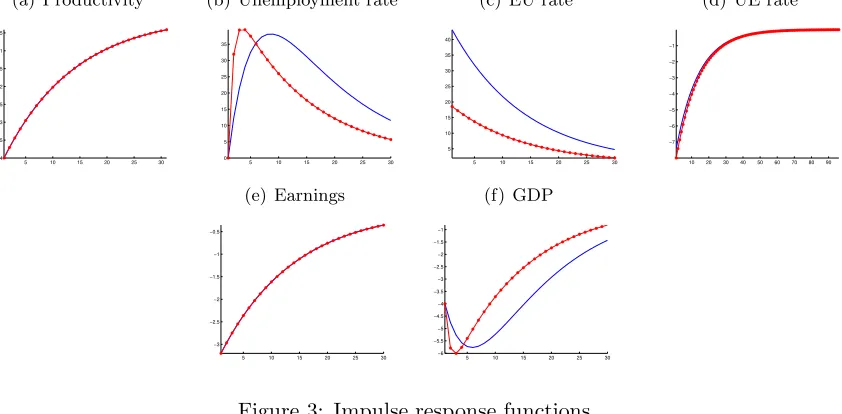
The difference in the reaction of the unemployment rate to shocks are not generated by differences in the reaction of wages. Despite the lower bargaining power in the U.S. the wage reaction was targeted to be the same across the two countries, and is confirmed in figure 3(e). The difference is also not due to differences in the UE reaction given that the reaction is almost identical in both countries (figure 3(d)). What causes the sluggish response in Germany is an interplay of the strong reaction in the EU rate causing a strong rise in unemployment (figure 3(c)) and the low reemployment probabilities due to the lower average UE rate caused by the lower matching efficiency in Germany. The low reemployment probability in Germany leads to a situation where we observe output growth after 6 quarters in combination with increasing unemployment rates for additional 3-4 quarters. For large shocks such a recovery might therefore well look like a period of a jobless recovery Shimer (2010).
5
Additional Explanations and Robustness
(a) Productivity
5 10 15 20 25 30 −4 −3.5 −3 −2.5 −2 −1.5 −1 −0.5
(b) Unemployment rate
5 10 15 20 25 30 0 5 10 15 20 25 30 35
(c) EU rate
5 10 15 20 25 30 5 10 15 20 25 30 35 40
(d) UE rate
10 20 30 40 50 60 70 80 90 −7 −6 −5 −4 −3 −2 −1 (e) Earnings
5 10 15 20 25 30 −3 −2.5 −2 −1.5 −1 −0.5 (f) GDP
[image:22.612.99.520.26.233.2]5 10 15 20 25 30 −6 −5.5 −5 −4.5 −4 −3.5 −3 −2.5 −2 −1.5 −1
Figure 3: Impulse response functions
Notes: The figure plots the impulse response functions for the U.S. (red dotted lines) and Germany (blue solid line) on a quarterly scale.
differentially. This effect might give firms incentives to circumvent firing taxes for low tenured workers using for example short-term employment contracts Costain, Jimeno, and Thomas (2010); Bentolila, Cahuc, Dolado, and Barbanchon (2010).
In this section we examine whether similar mechanisms could also explain the stylized facts for the cross-country differences between Germany and the U.S. For this purpose we first present empirical results for the labor market dynamics in Germany controlling for tenure. We then offer a theoretical exploration based on the augmented model with idiosyncratic shocks that uses our empirical findings to discriminate between these alternative explanations.
5.1 Tenure - Data
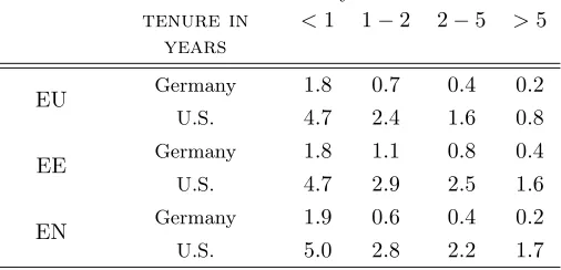
To examine the role of skill accumulation and employment protection empirically we construct transition rates conditioning on tenure for four tenure classes. For Germany this data can be constructed from the employment histories. For the U.S. we rely on irregular supplements to the CPS that report information on tenure with the current employer.28 For both countries we report in Table 7 time averages of monthly rates across all available observations.
We find that both countries show a strongly declining pattern of transition rates with tenure. This holds for all separation rates either to a new firm, to unemployment or to inactivity. In Germany
28We use theOccupational Mobility and Job Tenure supplements for the years 1983, 1987, 1991, 1996, 1998, 2000,
the average rates are substantially below the U.S. rates in all tenure classes. However, the decline across tenure groups is very similar in the two countries. In both countries the share of low tenured worker29in all EU transitions is larger than 50% but is a bit smaller in the U.S. (60%) compared to
[image:23.612.180.433.116.238.2]Germany (72%). For Germany we can also look at the volatilities of transition rates across tenure
Table 7: Transition rates by tenure classes
tenure in years
<1 1−2 2−5 >5
EU Germany 1.8 0.7 0.4 0.2
U.S. 4.7 2.4 1.6 0.8
EE Germany 1.8 1.1 0.8 0.4
U.S. 4.7 2.9 2.5 1.6
EN Germany 1.9 0.6 0.4 0.2
U.S. 5.0 2.8 2.2 1.7
Notes: Tenure categories are given in years. All transition rates are given as percentages of the workers in the respective tenure group and are averages over time. For Germany only workers in full-time employment over the period 1980−2004 are considered. The U.S. rates are derived using the January and February supplements to the Current Population survey (CPS) using available supplements in the period 1983−2006. Due to the rotation of the panel and the point in time information on tenure in the CPS, we report only transition rates in the month were tenure is available. U.S. transition rates are adjusted for seasonal effects and time aggregation to match their unconditional averages. The transition rates for Germany are constructed from employment histories and seasonally adjusted.
classes.30 Interestingly, we find that the EU rate volatility is very large for all tenure classes and is, if anything, increasing over tenure.31 We conclude from these observations that our findings of
substantially larger EU rate volatilities is not driven by low tenured workers moving in and out of employment alone but that this facts holds more broadly over tenure classes.
5.2 Augmented Model
To investigate whether differences in the human capital accumulation process or differential firing taxes are major drivers of the labor market differences pointed out in section 2 we augment our benchmark model to allow for worker and match-specific human capital accumulation. To econ-omize on the state space, we assume that employed workers can be in three tenure states, low, medium and high (L, M, H). We assume that workers stochastically gain match-specific skills by staying at their firm, i.e. accumulating tenure. We normalize the initial state and set match specific productivity in the lowest tenure state to sL = 1. The worker needs on average 2 years to transit
29We define low tenured as tenure below 2 years.
30Since we only have information at a limited set of points in time for the U.S., we can not calculate reasonable
volatilities for the different tenure classes there.
31The exact numbers for the standard deviations are 19.6, 17.4, 23.0, 23.4 where the first number refers to the
to tenure level M, and another three years to transit to the final tenure state H. Workers with 2−5 years of tenure (state M) have a skill level sM = (1 +gM) and workers with 5 years or more of tenure (state L) have skill level sH = (1 +gH). Upon separation the worker loses tenure. We target gM and gH to reproduce the declining EU transition rates in the United States. We find gM = 0.034 andgH = 0.067 so the yearly increase of skills in tenure is roughly 1.3%.32.
To study skill losses we additionally assume that the worker can be in one of three worker specific skill states, namely bad, normal, or good with productivity denoted byzB,zN, andzG respectively, so that the total number of idiosyncratic productivity states is nine. We assume that the skill process attached to the workerziis given by a discrete approximation to an AR(1) process with three states.33 We set the autocorrelation coefficient at 0.98 on a monthly basis to generate a persistent process as in Costain, Jimeno, and Thomas (2010) and set the standard deviation to imply a shock size of 10% in our discrete approximation, normalizingzN = 1.34 Upon unemployment the workers also switch states according to this AR(1) process, so we have to keep track of the distribution of employed worker by skill and tenure level and unemployed worker by skill level.
Worker and match-specific transitions follow independent stochastic processes, so we calculate the appropriate transitions functions pee, peu,pue and puu on the stacked vector of idiosyncratic states as the convolution of the two processes and assume that a particular individual state is the multiplication of the two processes.35 We aggregate over the worker specific states and report the
average for each tenure class.
We re-calibrate the remaining parameters to match the same aggregate statistics as in the bench-mark case.36 The upper part of Table 8 reports the calibrated U.S. economy together with the
empirical targets. The last line in the upper part reports the data targets for Germany. In the lower part of the table we perform foure experiments similar to the ones in table 6. Again, we change parameters (first column) starting from the calibrated U.S. economy to match a German data target (bold number).37
32Altonji and Williams (2005) reports gain to tenure of 11% for ten years for the U.S., roughly in line with these
numbers. Dustmann and Meghir (2005) report returns to tenure for skilled German worker between 1.7−2.4%.
33We use the method of Kopecky and Suen (2010) to obtain the conditional Markov transition kernel numerically.
34In contrast to standard models with endogenous destruction the variance of the worker specific shock process is
less important for the business cycle dynamics given that separation rates are still governed by idiosyncratic match specific shocks with variance proportional toψwhich we again calibrate to reproduce the aggregate EU rate volatility of the U.S.. We varied the standard deviation between 5−20% and re-calibratedψwithout affecting the results.
35That is the first state isx
1 =sLzB, x2 =sLzN, . . . , x9 =sHzG. The resulting transition matrix pue(x, x′) for
example takes care of the fact that unemployed workers can only switch to low tenured jobs.
36We additionally introduce a stochastic probability of retiring to generate the tenure distribution. We set the
work-life to 40 years as in as in Costain, Jimeno, and Thomas (2010) and assume that newly born workers are born with skill levels according to the invariant distribution of the Markov transition. We adjust the model equation accordingly. We see that heterogeneity lowers the average net replacement rate, but only very modestly. All other parameters are very similar to the benchmark case. This results for the U.S. economy in the following parameters
κ= 0.26,κ= 0.52,µ= 0.35,ψ= 1.08, b
w = 0.926, andτ = 3.05.
37We rely numerically throughout on a first order approximation, given that the state space has to include all
Table 8: Experiments
πEU,L πeu,M πeu,H πue σ˜ue σ˜eu,L σ˜eu,M σ˜eu,H σw
U.S. (Data) 3.55 1.68 0.8 30.6 11.2 *6.5* 0.8 U.S. (Model) 3.55 1.68 0.8 30.6 11.2 4.6 5.8 6.7 0.8 GER (Data) 1.3 0.4 0.2 6.2 10.5 18.4 23.5 23.4 0.8 (1) κ= 0.12 1.4 0.5 0.2 6.2 10.1 14.6 16.8 19.1 0.67 (2) τM, τH= 4.9 3.7 0.4 0.2 28.9 14.3 5.2 9.0 10.0 0.82
(3) τM, τH= 4.5 2.9 0.4 0.2 6.2 12 8.0 12.6 14.5 0.94 µ= 0.92
(4) Turbulence 2.6 0.9 0.4 21.5 19 6.4 9.1 12.3 0.85
Notes: The upper part reports the data. The lower part reports the experiments. πeu,L,πeu,M and πeu,H denotes
the EU rate for low (medium, high) tenured worker averaged over all idiosyncratic skill levels. The same applies for ˜
σeu. The value on the EU rate volatility for the U.S. marked by * is the average over all tenure classes due to data
limitations.
5.2.1 Matching Efficiency Revisited
The first experiment decreases the matching efficiency (κ) to show that the identified mechanism
from the previous section still works in the extended model. The average UE rate falls. The surplus in each tenure class increases in Germany due to the lower average UE rates, so accumulated skills get more valuable. Upon separation high tenured workers will lose their tenure. Due to the long search duration it takes longer to accumulate human capital in a new match which makes German workers more reluctant to separate. The average EU rates fall in a way consistent with the observed tenure patter. Moreover, due to the larger surplus in each tenure class the EU rate volatilities increase.
5.2.2 Differential Firing Taxes
If differential firing taxes were an important driving force of the cross-country difference, one might suspect that short-term employment contracts would be one possibility to circumvent this friction.38
To shed light on this alternative explanation we use in the second and third experiment differential firing taxes to explain the decline in Germany for higher tenured worker. We keep τL at its U.S. value and increaseτM and τH to target the observed EU rates in Germany. We see in experiment 2 that the presence of tenure dependent firing taxes lead to a decline in the EU rates for protected workers and to an increase for unprotected workers. The EU rate volatility modestly increases for higher tenured workers due to a larger surplus, and remains largely unchanged for low tenured worker. The unemployment volatility is amplified because both the UE rate as well as the EU rate
38There is no direct evidence that short-term employment contracts increased substantially in Germany during the
volatility increase. The contribution of the EU rate volatility though falls because the increase in the UE rate volatility dominates, in line with our findings for the benchmark model.
A firing tax by itself has only a very small impact on the average UE rate. If firing taxes affect in addition the threat point of the bargaining, the implicit bargaining power increases. The third experiment varies therefore jointly the firing taxes as well as workers bargaining power. As analyzed before, a substantial increase in the bargaining power will raise the surplus, if the deviation from the Hosios condition is large enough (we need aµ= 0.92). Again, we would see a larger decline in the EU rates for high tenured workers by construction, a counterfactually high average EU rate for low tenured workers and a counterfactually low EU rate volatility. Moreover, the surplus of new hires tends to decline, increasing the UE rate volatility.
5.2.3 Human Capital Accumulation and Turbulence
The final experiment considers a version of turbulence along the lines of Ljungqvist and Sargent (2008) to study the role of worker and firm specific human capital. We assume that skills are more firm specific in Germany and might be lost after a separation. Concretely, we assume that workers with a good skill level lose their skills and become a normal type upon separation, while workers with normal skill level become bad types. That is a large fraction of the work force lose 10% of their skill level upon separation. This assumption transforms skills that are attached to the worker in the U.S. to skills that are more specific to the match in Germany. 39
As a consequence of the higher risk of losing skills the surplus for medium and high skilled workers increases due to the deterioration of the outside opportunity. As a result the average EU rates decline for these groups. For low tenured workers the decline is not as pronounced as observed in the data. Two effects are at work: The increase in the average surplus tends to increase the average UE rate making it more attractive for firms to post vacancies because there is more to split. However, the composition of the unemployment pool changes. There are more bad types in the search pool, making it less attractive to post vacancies. In our calibration there are 44% bad types in the unemployment pool for the U.S. while in Germany, due to the skill losses, the number increases to 75%. If differences in the skill processes were the main driving force in explaining the empirical labor market differences, the deterioration of skill effect has necessarily to dominate to explain the low average UE rates observed in Germany as it does on our calibration. However, the resulting decline in the expected surplus from creating an open position implies that the UE rate volatility will increase and we find a counterfactual decline in the contribution of the EU flows relative to the UE flows in the unemployment volatility.
Our experiments show that the behavior of the transitions rates by tenure are potentially
infor-39We choose this calibration that is at the upper end of empirically plausible values (Fujita (2008), Burda and
mative to discriminate between different explanations studied in the literature. Differential firing taxes do not explain the low average transition rates of low tenured workers in Germany which should be less affected by firing restrictions. Differences in the idiosyncratic skill processes either increase the surplus, if they lead to more match specific skills in Germany, or decrease the expected surplus, if the cost to re-training low tenured workers is large or the search pool has very bad skills. In the former case the average UE rate should increase, because firms can exploit the worker better, in the latter case the contribution of the UE rate volatility would increase. Both implications are counter-factual. To explain the data one needs a mechanism that jointly increases the surplus and lowers the average UE rate.
Our quantitative results so far have relied on the small surplus calibration of Hagedorn and Manovskii (2008). We now show that our results still hold under an alternative set of assump-tions that allow for a larger surplus calibration and study the impact of wage rigidities on the volatilities.
5.3 Rigid Earnings
The recent literature has stressed versions of wage rigidities as a potentially important source of an amplification mechanism that can explain the large hiring rate volatilities without relying on an outside option close to productivity (Shimer (2005), Hall (2005) and more recently Elsby and Michaels (2010)). Maybe surprisingly, we find empirically that German earnings40 are not any
more rigid in Germany compared to the U.S., though confidence bands are large. We show on theoretical grounds that strong versions of wage rigidity will affect the EU rate and the UE rate volatility symmetrically, leaving the contribution rate to the unemployment volatility unaffected.
5.3.1 Empirical Estimates
As an empirical measure of earning rigidity the literature typically uses an elasticity estimate on the reaction of wages or earnings with respect to a measure of the business cycle. As this measure of business cycle either productivity or the unemployment rate have been used.
These studies also differ in the way how they control for selection effects. Several approaches have been proposed to control for this composition bias. Following Solon, Barsky, and Parker (1994) we use a fixed group of individuals of continuously employed workers who stayed at the same firm over the whole sample period. This selection rules out work force composition effects because the composition of the group is fixed in terms of all observable characteristics.41 The drawback of this
40We focus on earnings because our dataset does not have an hours worked measure. The online appendix documents
that our earnings measure and aggregate measures of wages move almost one to one, and that the behavior of hours worked is likely not an important source of the cycle variation of earnings in Germany.
41This group is informative about the cyclicality of earnings because if repeated annual collective bargaining about