ISSN Online: 2163-0437 ISSN Print: 2163-0429
DIMZAL: A Software Tool to Compute
Acceptable Safety Distance
Paul-Antoine Bisgambiglia, Jean-Louis Rossi, Romain Franceschini, François-Joseph Chatelon,
Paul Antoine Bisgambiglia, Lucile Rossi, Thierry Marcelli
University of Corsica, Corte, France
Abstract
The scope of this work is to present a multidisciplinary study in order to propose a tool called DIMZAL. DIMZAL forecasts fuelbreak safety zone sizes. To evaluate a safety zone and to prevent injury, the Acceptable Safety Distance (ASD) between the fire and firefighters is required. This distance is usually set thanks to a general rule-of-thumb: it should be at least 4 times the maximum flame length. A common assumption considers an empirical relationship between fireline intensity and flame length. In the current work which follows on from an oral presentation held at the VII International Conference on Forest Fire Research in Coimbra in 2014, an alter-native way is proposed: a closed physical model is applied in order to quantize the ASD. This model is integrated in a software tool, which uses a simulation framework based on Discrete EVent system Specification formalism (DEVS), a 3D physical real- time model of surface fires developed at the University of Corsica and a mobile ap-plication based on a Google SDK to display the results.
Keywords
Decision-Making Tool, Fire Model, Acceptable Safety Distance, ASD, Calculation Tool, DEVS, Mobile Application
1. Introduction
Physical models are based on mathematical analysis of the fundamental physical and chemical processes, which control forest fires. Mathematical expressions are generated from the laws that govern combustion, fluid mechanics and heat transfer. Due to the complexity of fire mechanisms, models have been carried out with different degrees of simplification from empirical approaches to software packages implementing computa-tional fluid dynamics of reacting flow (Harzallah et al., 2008). For example, the DEVS formalism has been used to model chemical and physical equations describing fire propagation (Muzy et al., 2002; Bisgambiglia et al., 2006; Harzallah et al., 2008; Nader et
How to cite this paper: Bisgambiglia, P.-A., Rossi, J.-L., Franceschini, R., Chate-lon, F.-J., Bisgambiglia, P. A., Rossi, L., & Marcelli, T. (2017). DIMZAL: A Software Tool to Compute Acceptable Safety Dis-tance. Open Journal of Forestry, 7, 11-33. http://dx.doi.org/10.4236/ojf.2017.71002
Received: October 11, 2016 Accepted: December 23, 2016 Published:December 26, 2016
Copyright © 2017 by authors and Scientific Research Publishing Inc. This work is licensed under the Creative Commons Attribution International License (CC BY 4.0).
http://creativecommons.org/licenses/by/4.0/
al., 2011). This article deals with a multidisciplinary work involving searchers in com-puter science, in physics and mathematics in order to develop a simple tool that fore-casts safety zone sizes at the field scale (DIMZAL) (Bisgambiglia et al., 2014).
Wildland fires represent a growing threat on human infrastructure and activities par-ticularly due to the spreading of the Wildland-Urban Interface. From a fire safety point of view, the fire has two main impacts: it can damage structures and affect people. Par-ticularly, firefighters wearing protective equipment have to remain at a close distance from the fire front to fight against it and not too close in order to keep safe (Butler, 2014). In this work, a mobile application that determines safety zone sizes at the field scale as a function of fire environment and fuel characteristics is proposed.
Wildland fires result in moderate to high rates of spread and intensities and they can burn easily a few days after heavy rainfall (Morandini et al., 2006; Santoni et al., 2006). For instance, these fires occur in fuel type like Shrubland. This combustible has high flammability. Thus there is a pressing need to produce an accurate evaluation of the distance between the fire and men required to prevent injury during operational phas-es. Actually, safety distances are always defined to have some space between the fire and the different types of targets (Zárate et al., 2008; Rossi et al., 2011).
For many of the regulations and standards used throughout the world, the criteria for human exposure are specified only by heat flux magnitude (Raj, 2008). One can no-tice that logically time of exposure is also critical (Eisenberg et al., 1979). Commonly, in operational conditions, a rule-of-thumb is applied to determine this safety distance: the distance between the fire and the firefighters should be at least 4 times the maximum flame length(Butler & Cohen, 1998). A common assumption consists of using an em-pirical relationship between fireline intensity and flame length. So, several works have established empirical correlations between fireline intensity (fireline intensity is the rate of heat release per unit length of fire line) and time average flame length (van Wilgen et al., 1985; Vega et al., 1998). They were estimated using statistical fitting procedures. The use of these relationships needs a solid understanding of the limitations of these models and this precludes an empirical approach to evaluate safety distances in fuel types, which are structurally very different (Morvan et al., 2002). This is a strong argument for the simplified physical approach developed in this study.
For several years, the fire team of the university of Corsica works on a fire models set (Balbi et al., 2007, 2009, 2010). These different models are used to fire studies at differ-ent detailed levels, from fire laboratory to real forest fire. Recdiffer-ently, some models have been developed to compute safety distance (Butler, 2014). In this work, its integration is proposed into an online calculator: a Web Service. This web service will be interrogated by a mobile application to provide an acceptable safety distance defined from a geo-graphical area (GIS: Geogeo-graphical Information System). DIMZAL has been designed with and for firefighters, to meet their needs. A mobile application is of great interest because it is portable and allows you to go on the ground.
such as vegetation, meteorology, topography, etc. In forest fires research literature, it is generally admitted that the radiation from flames is the dominant mechanism of fuel bed preheating. So the flame is commonly modeled as a radiant surface with a given height, constant temperature and emissivity. This approach is generalized to take into account the effect of the fire front width. In this first part the DEVS formalism pro-posed is presented too. The formalism selected is called DEVS for Discrete Event
sys-tem Specification; it can be defined as multi-formalism and used as a computational
tool. In the field of Discrete Event Systems (DES), many efforts have been devoted to develop appropriate tools to study, and model in a formal way the dynamics and the mechanisms of interaction of the natural systems. For several years the community is changing DEVS formalism so that it can become a powerful tool for modeling com-plex systems. DEVS allows the reusing models through library already developed and also interconnecting of these models to compose heterogeneous models based on dif-ferent formalisms. Its advantage is to open the application to fields such as web appli-cations or Web Services.
In the second part, flame length model prediction has been compared against empir-ical laws using experimental outdoor fires. These results show that the simplified phys-ical approach presents a main advantage: its capability to be used for all types of fires under a wide range of conditions. So, the physical flame model can be seen as an alter-native operational flame length model, which can be applied to calculate more accu-rately safety distances.
In the third part, a detail of the software architecture is done (Bisgambiglia et al., 2013). The mobile application is detailed and its GUI (graphical user interface). Fire models have been implemented in a DEVS framework and coupled with a computa-tional model of acceptable safety distance (ASD). The simulator is hosted on a Server to be queried remotely. At the start of the process, the user sends to the server a message with several positions. The server queries the Web Services to determine local parame-ters (slope, wind, etc.), and for each position compute the ASD. Finally, results are re-turned to the client for visualization in GIS. In the third part, some results are described and commented. Computation of Acceptable Safety Distances in which a fire spreads across five different fuels in the Mediterranean area is presented and a final result is shown too.
2. Models
In the last few years the increasing influence of global warming on the environment has produced periods of drought, which in turn have led to wildfires with devastating con-sequences. There is a growing need for firefighters to have decision-making tools (Butler, 2014). However, wildfires are so unpredictable that reducing their impact is still a complex task. A broad range of conditions can cause firefighter entrapment and injuries. The main question associated with the safety of firefighters is: how to define wildland firefighter safety zones?
2.1. Acceptable Safety Distance and Fuelbreak
Distance (ASD) between the fire front and men to prevent injury. This problem can be divided into two topics area: 1) determination of the fire intensity and 2) calculation of distance from the fire to prevent injury. This section sets out each of these topic areas.
2.2. Determination of Fire Intensity
Fireline intensity is calculated by Byram’s equation (Byram, 1959):
B c a
I = ∆H w R (1) where ∆Hc is the heat yield of the fuel; wa is the weight of fuel consumed in the ac-tive flaming front and R is the rate of spread. This expression defines fire intensity as the rate of heat energy released per unit time and unit length of fire front, the latter be-ing considered regardless of the fire front width. This approach to determinbe-ing the fire-line intensity has been commonly used around the globe since 1959 (Higgins et al., 2008).
2.3. Calculation of the Acceptable Safety Distance (ASD)
Energy is transferred in wildland fires mainly by two prevalent heating modes: radia-tion and convecradia-tion. It is generally admitted that radiaradia-tion dominates the heat transfer process. In order to evaluate the ASD, empirical relationships or simplified physical models can be applied.
2.3.1. Empirical Law
Commonly, in operational conditions, a rule-of-thumb is applied to determine the ac-ceptable safety distance: the distance between the fire and the firefighters should be at least 4 times the maximum flame length (Butler & Cohen, 1998)
4 f
ASD= l (2)
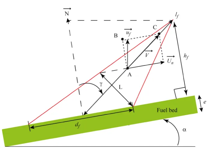
[image:4.595.200.550.473.720.2]where lf is the flame length as illustrated in Figure 1.
Flame length (cf. Figure 1) is the most obvious manifestation of heat release and is frequently the preferred descriptor of flame size (Fernandes et al., 2009). So, several works have established empirical correlations between fireline intensity and flame length at the field scale (Nelson Jr. & Adkins, 1986; Burrows, 1994; Butler et al., 2004; Fernandes et al., 2009). These relationships are of the form of a power function of flame length fitted to Byram’s intensity:
b
f B
l =aI (3) where IB is the fireline intensity, a and b two fitted model parameters.
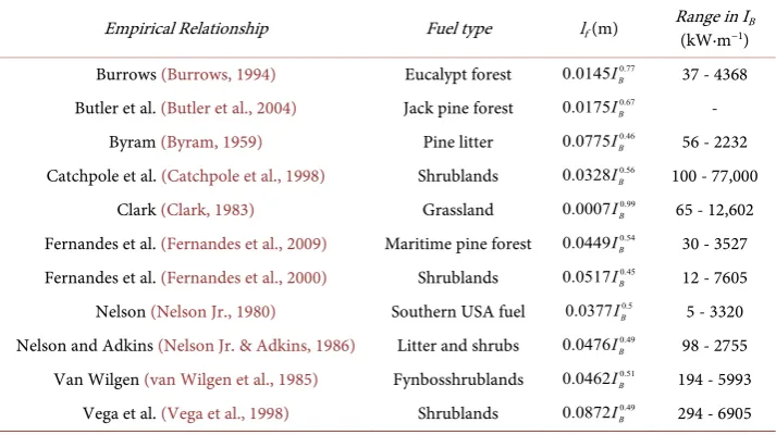
The values of the model’s parameters are always estimated using statistical fitting procedures from experimental data in the field. Consequently, different values are pro-duced from different fuels. Moreover, one can note that the use of these relationships needs a solid understanding of the limitations of these models (Alexander & Cruz, 2012). A selection of these laws used at the field scale and their limitations are summa-rized in Table 1.
Nevertheless, despite the fact that the relationship (2) is always developed from ex-perimental studies in a single fuel type, many operational users of fire modeling sys-tems have come to view it as universal in nature (Andrews et al., 2011).
2.3.2. Analytical Approach
At the University of Corsica, a simplified physical approach, which consists in coupling a simplified physical propagation model with a flame length sub model and an opera-tional relationship for the safety distance is proposed. The propagation model (Balbi et al., 2007, 2009, 2010) is constituted by several equations and the two main equations giving the rate of spread (R) are:
0
0
0
tan tan
1 sin cos cos 1
n U
u
R R AR R
[image:5.595.196.553.538.738.2]r γ α γ γ γ = + + − = + + (4)
Table 1. Listing of some empirical laws described by relationship (3).
Empirical Relationship Fuel type lf (m) Range in I(kW∙m−1) B
Burrows (Burrows, 1994) Eucalypt forest 0.0145 0.77 B
I 37 - 4368
Butler et al. (Butler et al., 2004) Jack pine forest 0.0175 0.67 B
I -
Byram (Byram, 1959) Pine litter 0.0775 0.46 B
I 56 - 2232 Catchpole et al. (Catchpole et al., 1998) Shrublands 0.0328 0.56
B
I 100 - 77,000 Clark (Clark, 1983) Grassland 0.0007 0.99
B
I 65 - 12,602 Fernandes et al. (Fernandes et al., 2009) Maritime pine forest 0.0449 0.54
B
I 30 - 3527 Fernandes et al. (Fernandes et al., 2000) Shrublands 0.0517 0.45
B
I 12 - 7605 Nelson (Nelson Jr., 1980) Southern USA fuel 0.0377 0.5
B
I 5 - 3320 Nelson and Adkins (Nelson Jr. & Adkins, 1986) Litter and shrubs 0.0476 0.49
B
I 98 - 2755 Van Wilgen (van Wilgen et al., 1985) Fynbosshrublands 0.0462 0.51
B
I 194 - 5993 Vega et al. (Vega et al., 1998) Shrublands 0.0872 0.49
B
In the first equation, the flame tilt angle (γ) depends on the terrain slope angle (α), the normal component of the wind speed (Un) and the upward gas velocity (uo). The
second equation is the sum of two terms. The first one, Ro, evaluates the rate of spread
under no wind and no slope (it represents the contribution of the radiation from the fuel burning particles area). The second one determines the radiant heat flux, which comes from the flame body.
A flame height submodel (Marcelli et al., 2011) is added to the simplified physical rate of spread model described by Equation (4). As hf = lfcosγ where lf and hf denote the
flame length and the flame height respectively, the flame length is expressed as
0 00 4
2
cos v
f
f
r H l
BT
χ ρ ν
γ ∆
= (5)
where χ0 is a radiant factor (usually close to 0.3); r00 is a universal rate of spread (ROS)
factor (equal to 2.5 × 10⁻⁵); ΔH is the heat of combustion of the pyrolysis gases; ρ v is the
fuel density; ν is the fuel absorption coefficient; B is the Stefan-Boltzmann constant and
Tf is the mean flame temperature.
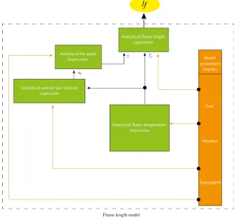
Three other analytical expressions (Balbi et al., 2010) are necessary to calculate the flame length if some parameters are available (fuel, weather and topographic characte-ristics): the upward gas velocity at mid-height flame (u0), the flame temperature (Tf)
[image:6.595.204.543.401.715.2]and tilt angle (γ). One can note that an accurate knowledge of these characteristics is mandatory to obtain a proper value of the flame length. Physical model processes are summarized in Figure 2.
Finally, flame characteristics are inserted into an analytical relationship, which allows the calculation of acceptable safety distances (Rossi et al., 2011):
1WI 1 exp thres2 f L
ASD ASD k
l
= − −
(6)
with
(
4)
21
cos 4
sin 2
f thres f thres f
WI
f thres
l l BT
ASD = Φ γ − Φ + ετ +l γ
Φ (7)
where kthres is an empirical parameter that must be determined for each selected
thre-shold of the heat flux; Φthres is the threshold heat flux level; τ is the atmospheric transmissivity; ε is the equivalent flame emissivity; B is the Stephan-Boltzmann con-stant and Tf is the flame average temperature. There is one important thing in this
formula: the model takes into account the threshold heat flux level.
2.3.3. Fuelbreak Dimension
Fuelbreaks divide expanses of natural fuels into smaller units. Native vegetation on these strategically located wide strips of lands is modified so that fire burning into them can be more readily and safely controlled. Fuelbreak generally has a low-growing ground in order to protect the soil against erosion. But, fuelbreaks with safety zones providing safety for firefighting personnel and equipment under critical conditions should be wider than other parts of a fuel break. In selecting the widths of fuelbreaks safety zone, the forest manager must estimate the distance from the flame front neces-sary to prevent serious burns from radiated heat and direct ignition from radiation too. (Green & Schimke, 1971) estimated that the distances from the flame front necessary to prevent ignition from radiation are half of the distances considered necessary to pre-vent disabling burns. Hence, ignition from radiation across a wide fuelbreak should not be a problem. Assuming that the safety distance is in the center of the break, the total width of a fuelbreak safety zone must be equal to 2 times this distance.
2.4. DEVS Formalism
Since the 1970s, with the advances in computing speed, storage capacity and graphical capabilities, several integrated fire prediction systems have been developed. DIMZAL uses the Discrete Event System Specifications (DEVS) formalism (Ziegler et al., 2000). DEVS is an algebraic formalism to explicitly represent Discrete-Event Systems (DES), Discrete-Time Systems (DTSS). The semantics of the abstract simulator gives a unique interpretation of a DEVS model, increasing the power of this modular and hierarchical formalism. This formalism allowing accurately phrases the behaviour complexity of a real system of various domains and situations. It constitutes a simulation paradigm in complex system science. DEVS allows the complexity of real systems to emerge from a simplified description. ADEVS atomic model is based on:
Continuous time.
Inputs, outputs and states.
Complex models are constructed by connecting several atomic models in a hierar-chical way. The interactions are established using the models’ input and output ports, which favours modularity.Although a variety of simulation models based on this for-malism have been performed simulating wildfire spread requires several evolutions of this fundamental computational structure. This work is proposed to modify the basic approach.
A DEVS model incorporates one or more atomic model (AM). (AM) gives an inde-pendent description of the system’s behaviour. An atomic model is described by the following expression:
: ; ; ; ;a ext; int;
AM X Y S t δ δ λ (8)
where,
X = {(pin, v)|pin⋲ Input ports, v Є Xpin}: list of the model inputs;
Y = {(pout, v)|pout⋲ Output ports, v Є Ypout}: the list of the model outputs;
S: state variables;
ta: S ⟶R+: time advancement function;
δext: QxX ⟶S: external transition function; δint: S ⟶S: internal transition function;
and,
λ: S ⟶Y: output function.
Why DEVS? This approach is mainly used to its openness and extensibility. For ex-ample, comparisons between tests using the physical models presented hereby calcu-lated with a conventional software tools (software Mathematica®) and this DEVS for-malism, give the same results. Its advantage is to open the application to other fields such as web applications or Web Services. Mapping DEVS models in Web Services is the subject of many current approaches (Kim & Kang, 2005; Mittal et al., 2007; Seo & Ziegler, 2012). The aim of this works is: 1) to provide a service based on a DEVS model, and 2) to extend the interoperability of DEVS formalism. This work must be considered as a simply use of these concepts applied to a specific case: the determination of the ASD. The selected approach is usual because DEVS is applied as a calculation tool. In addition, DEVS can be used to transform this calculation tool in an online tool. So, this tool can be seen as complete software architecture; efficient and adapted to this par-ticular problem: proposing a portable field tool for fuelbreak dimensioning.
3. Confrontation of Physical Flame Models with Experiments
3.1. Fire Tunnel Experiments
The first set of experiments data concerns the burning of Quercus coccifera fuel in the presence of an aiding wind (0, 0.5, 1, 1.5, 3 and 5 m∙s−1). Six fire experiments have been
realized in a fire tunnel located in south of France (Marseille). The load was fixed at 3 kg∙m−2 for Quercus coccifera with an average thickness of 0.9 m. Four more fire
expe-riments have been carried out with a 5 kg∙m−2 fuel load. The experimental apparatus
was composed by a visual video camera (30 images/second, 640 × 480 pixels). The de-tailed experiment methodology is presented in (Chetehouna et al., 2008).
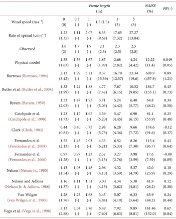
[image:9.595.199.551.296.733.2]The Fernandes’ law (Fernandes et al., 2000) and the Physical model present the smallest NMSE (cf. Table 2). So, these models give accurate results for this particular set of laboratory experiments. The ten other relationships give an overprediction of the flame length.
Table 2. Observed and predicted flame lengths during the laboratory scale experiments with a 3 kg∙m−2 fuel load (5 kg∙m−2 fuel load).
Flame length
(m) NMSE (%) FB (-)
Wind speed (m·s−1) 0
(0) 0.5 (-) (-) 1.5 (1.5) 1 (3) 3 (5) 5
Rate of spread (cm·s−1) 1.22
(1.35) 1.11 (-) 2.07 (-) (9.68) 8.33 (7.32) 17.65 (13.04) 27.27
Observed 1.6 (2) 1.7 (-) 1.9 (-) (2.3) 2.1 (2.5) 2.3 (2.8) 2.5
Physical model (1.63) 1.55 1.56 (-) 1.67 (-) (1.99) 1.85 (2.82) 2.68 (4.42) 4.24 (11.4) 12.22 (0.05) 0.049
Burrows (Burrows, 1994) (3.42) 2.13 1.99 (-) 3.21 (-) (15.59) 9.37 (12.57) 16.70 (19.6) 23.34 (457.9) 608.9 (1.21) 0.89
Butler et al. (Butler et al., 2004) (1.99) 1.32 1.24 (-) 1.88 (-) (7.42) 4.77 (6.15) 7.87 (9.05) 10.52 (133.1) 184.7 (0.73) 0.43
Byram (Byram, 1959) (2.03) 1.53 1.47 (-) 1.95 (-) (5.03) 3.71 (4.42) 5.24 (5.77) 6.40 (48.2) 64.8 (0.50) 0.34
Catchpole et al.
(Catchpole et al., 1998) (1.73) 1.23 1.17 (-) 1.65 (-) (5.20) 3.59 (4.45) 5.47 (6.15) 6.98 (55.9) 81.1 (0.48) 0.25
Clark (Clark, 1983) (0.81) 0.44 0.40 (-) 0.75 (-) (5.75) 2.98 (4.36) 6.28 (7.72) 9.66 (91.6) 174.6 (0.37) -0.12
Fernandes et al.
(Fernandes et al., 2009) (2.13) 1.52 1.45 (-) 2.03 (-) (6.21) 4.33 (5.33) 6.52 (7.30) 8.26 (86.7) 115.4 (0.64) 0.43 Fernandes et al.
(Fernandes et al., 2000) (1.28) 0.97 0.97 (-) 1.23 (-) (3.13) 2.32 (2.76) 3.27 (3.59) 3.98 (7.39) 17.6 (0.05) -0.08
Nelson (Nelson Jr., 1980) (1.54) 1.13 1.08 (-) 1.48 (-) (4.13) 2.96 (3.59) 4.32 (4.79) 5.37 (25.9) 42.0 (0.29) 0.10
Nelson and Adkins
(Nelson Jr. & Adkins, 1986) (1.57) 1.16 1.11 (-) 1.51 (-) (4.15) 3.00 (3.62) 4.34 (4.81) 5.38 (26.2) 41.9 (0.30) 0.12 Van Wilgen
(van Wilgen et al., 1985) (1.76) 1.28 1.23 (-) 1.68 (-) (4.84) 3.45 (4.19) 5.07 (5.64) 6.33 (44.2) 63.9 (0.44) 0.24
3.2. Literature Field Shrub Experiments
This section deals with the comparison of thirteen experimental literature field shrub-land fires with model results. Experiments were located in mountain areas in the southern Cape Province of South Africa. Fires were conducted at two sites. The first site is located in the Kogelberg State Forest (110 m above the sea level). This site is mainly level with a maximum slope of 6 degrees. The dominant tall shrub was Leucadendronl
aureolum and the understorey consisted of various Restionaceae, Cyperaceaea, and
fine-leaved shrubs of the families Asteraceaea. The second site is located in the Ceder-berg State Forest (470 m above the sea level). Plots inclinations ranged from 6 to 15 de-grees. Tall shrubs of the family Proteaceae predominated. The understorey consisted of various Restionaceae and Ponceae, and fine-leaved shrubs of the families Asteraceaea.
Kogelberg and Cederberg. The different small plots (about 50 × 50 m) were selected for apparent structural homogeneity of the vegetation (tall open shrubland, about 1 - 8 m). Despite the fact that sites were selected for their apparent structural homogeneity, there was considerable variation in the total fuel load (from 0.969 to 3.415 kg∙m−2). Air
tem-perature ranged from 13.9˚C to 38.3˚C, relative humidity from 15 to 90 % and mean wind speed from 1.03 to 3.56 m∙s−1. Detailed experiments description can be found in
(van Wilgen et al., 1985).
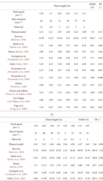
With regard to flame length models, four models are quite adequate to predict flame length in the Kogelberg (Table 3(a)) and the Cederberg experiments (Table 3(b)). These data are accurately fitted with the empirical relationships proposed by Fernan-des’, Nelson’s, Nelson and Adkins’s laws (Nelson Jr., 1980; Nelson Jr. & Adkins, 1986; Fernandes et al., 2000) and by the physical model too.
3.3. Field Shrub Experiments
In Corsica, Genista salzamannii constitutes a dense homogeneous layer of fine particles made of spines. The experiment was conducted by the Foresters of South-Corsica and is a part of a global soil occupation planning. A 1 ha plot was instrumented with ane- mometers and IR/Visible Cameras. The topography was established precisely and air humidity was measured. Vegetation sampling and analysis allowed a precise descrip-tion of the fuel before and after the fire (moisture content, dead and live particles ratio, elemental analysis). The experimental fire was carried out in October 2010 and the plot was situated at 1400 m above the sea level. Plot ignition was conditional of alignment between slope and wind direction. The selected plot was rectangular with a slope of 5 degrees. The average wind speed was equal to 2.22 m∙s−1. The fuel characteristics are
detailed in Table 4.
Two stereovision systems composed of two near infrared/visible cameras (JAI, 2009) rigidly fixed with a baseline of 1 m were used to estimate the flame length. One stereo-vision system was positioned in front of the fire along the fire propagation direction, at about 10 m of the limit of the fire propagation area. The other one was located in a lat-eral position relatively to the fire propagation direction.
Table 3. (a) Observed and predicted flame lengths during the Kogelberg State Forest experi-ments; (b) Observed and predicted flame lengths during the Cederberg State Forest experiments.
(a)
Flame length (m) NMSE (%) FB (-)
Wind speed
(m∙s−1) 3.56 1.5 2.67 2.67 3.11 3.11
Rate of spread
(cm·s−1) 44 36 21 30 37 47
Observed 3.2 2.4 2 4.3 3 4
Physical model 4.15 2.11 3.47 3.48 4.23 3.99 7.9 0.13 Burrows
(Burrows, 1994) 15.39 12.12 10.10 15.9 20.52 17.97 326.3 1.31
Butler et al.
(Butler et al., 2004) 7.33 5.96 5.09 7.55 9.41 8.39 80.1 0.80
Byram (Byram, 1959) 4.99 4.32 3.88 5.09 5.93 5.47 23.3 0.46 Catchpole et al.
(Catchpole et al., 1998) 5.15 4.33 3.80 5.28 6.35 5.77 27.1 0.49
Clark (Clark, 1983) 5.65 4.15 3.29 5.90 8.19 6.90 45.3 0.55 Fernandes et al.
(Fernandes et al., 2009) 6.15 5.20 4.57 6.30 7.54 6.87 48.6 0.65
Fernandes et al.
(Fernandes et al., 2000) 3.11 2.70 2.43 3.17 3.69 3.41 4.06 0.006
Nelson
(Nelson Jr., 1980) 4.09 3.50 3.11 4.18 4.94 4.53 9.57 0.27
Nelson and Adkins
(Nelson Jr. & Adkins, 1986) 4.12 3.53 3.14 4.20 4.95 4.55 9.84 0.28 Van Wilgen
(van Wilgen et al., 1985) 4.80 4.09 3.62 4.90 5.81 5.32 20.1 0.42
Vega et al.
(Vega et al., 1998) 7.54 6.47 5.76 7.70 9.07 8.33 82.6 0.82
(b)
Flame length (m) NMSE (%) FB (-) Wind speed
(m·s−1) 1.92 2.83 3.56 2.5 1.03 1.89 3.11 2.67
Rate of spread
(cm·s−1) 32 80 89 52 4 52 78 55
Observed 4 6 7 5 1.4 6.5 5 5
Physical model 4.52 5.27 6.65 4.84 3.94 3.99 6.27 5.63 7.66 0.09 Burrows
(Burrows, 1994) 17.55 59.03 45.32 19.23 3.78 26.40 40.38 33.34 582.9 1.33 Butler et al.
(Butler et al., 2004) 8.22 23.52 18.70 8.90 2.17 11.71 16.92 14.33 140.9 0.80 Byram
(Byram, 1959) 5.4 11.15 9.52 5.70 2.15 6.89 8.88 7.92 20.7 0.35 Catchpole et al.
Continued
Fernandes et al.
(Fernandes et al., 2009) 6.75 15.91 13.20 7.20 2.28 9.01 12.17 10.63 62.2 0.59 Fernandes et al.
(Fernandes et al., 2000) 3.36 6.87 5.88 3.55 1.36 4.28 5.59 4.91 5.48 -0.11 Nelson (Nelson Jr., 1980) 4.46 9.81 8.26 4.73 1.64 5.82 7.67 6.77 11.12 0.18
Nelson and Adkins
(Nelson Jr. & Adkins, 1986) 4.48 9.74 8.23 4.75 1.67 5.82 7.64 6.76 10.81 0.18 Van Wilgen
(van Wilgen et al., 1985) 5.23 11.76 9.86 5.57 1.88 6.87 9.13 8.03 24.03 0.34 Vega et al.
[image:12.595.196.553.88.229.2](Vega et al., 1998) 8.20 17.84 15.06 8.70 3.07 10.66 13.99 12.38 87.4 0.74
Table 4. Corsican mountain fuel characteristics.
Fuel (m) e ωrπ
(kg∙m−2) (%) m (J∙kgC−1p·K−1) (kg∙mρv−3) c
H
∆
(kJ∙kg−1·K−1) H
∆
(kJ∙kg−1·K−1) (msv−1)
Genista
salzamannii 0.48 0.2 8 1648 478 18620 14827 3100
near infrared images (Figure 3(a)) are not masked by smoke, have a shape very similar than in visible images (Figure 3(b)) and are more easy to segment (Rossi et al., 2014). That is the reason of the use of multimodal information to estimate the fire geometrical characteristics. The fire characteristics were calculated from three-dimensional coordi-nates of noticeable fire points computed using stereo image processing (Rossi et al., 2013).
It is clear that only three models show an adequate fitting to the observed flame length value (Table 5). The best fitting is founded using the physical model (NMSE =
0.35%and FB = 0.05) but the Burrow’s empirical law (NMSE = 6.9% and FB = −0.26) and the Vega’s empirical law also provide a correct fitting too (NMSE = 3.46%and FB = −0.18). In this specific case, the shrubland properties are all measured and the flame length is precisely measured using stereovision techniques. So, the physical model per-forms better than the eleven statistical models. One can note that it is a strong argu-ment for a simplified physical approach if the fuel is properly characterized.
The goal of this section is to provide an accurate flame length model at the field scale. To quantize the flame length different flame models (one simplified physical model and eleven empirical correlations) are tested using several experiments. Model predictions are only compared against measured flame length of spreading fires through shrub ve-getation. This work highlights that the simplified physical approach presents a main advantage: its capability to be used for all types of fires under a wide range of condi-tions if fuel models, describing structural types of vegetation, are available (Figure 4).
So, this model can be seen as an alternative operational flame length model, which can be applied to calculate more accurately safety distances.
4. Results and Web Service Implementation
(a) (b)
Figure 3. Images of a fire producing dense black smoke in the visible spectrum (a) and in the near infrared spectrum (b).
[image:13.595.205.540.259.480.2]Figure 4. Physical model results for all the experiments described herein.
Table 5. Computation of the ASD values (m) obtained with the physical model applied to five different fuels in the Mediterranean.
Wind
(m∙s−1) tall shrub Corsican Corsican shrub Sardinian shrub (type 1) Sardinian shrub (type 2) Grassland
3 10.14 11.16 11.05 10.48 8.86
5 14.87 16.06 20.46 15.32 14.37
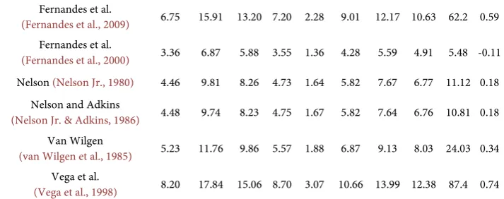
[image:13.595.193.555.546.613.2]Figure 5. An overview of the overall approach.
4.1. Mapping a Physical Model to a DEVS Model
The physical model is constituted by several equations and a large number of parame-ters. In order to solve these equations, the ASD evaluation is partitioned into five blocks. Then, these blocks are mapped into DEVS model.
Making model of ASD applying the DEVS formalism provides a coupled model composed of several sub-models. Once the dependency relationships are obtained, the ASD-DEVS models are built.
These models are implemented on a framework (Franceschini et al., 2014). A DEVS framework implement in C# language and, using simulation architecture called flat or direct (Franceschini & Bisgambiglia, 2014) coupling. Flat algorithms are presented in (Zacharewicz et al., 2010). The hierarchy of the simulation objects is flattened to reduce the communication overheads, using a flat simulation approach that eliminated the in-termediate coordinator, in order to reduce the time of simulation and to speed up the production of results. To validate the proposed model, comparisons were made with the original physical model ASD calculated in (Rossi et al., 2011) using the software
Mathematica®. The models were executed with multiple test cases and provided exactly
the same values. As the physical model under Mathematica® was validated by compari-son with experimental results (Rossi et al., 2011) this ASD-DEVS can be considered as conclusive. ASD model is composed of twenty-one distinct atomic models. Except the Generator each atomic model computes a specific equation for estimating the value 𝑥𝑥𝑖𝑖
associated with the model. The models are initially loaded by assigning arbitrary values to all variables except the constants and the fixed values like the Stefan-Boltzmann con-stant (B), the threshold heat flux level: (Φth), the local terrain slope angle (α) or the
am-bient temperature (Ta). A new value is computed for each 𝑥𝑥𝑖𝑖 variable by appropriated
atomic model. During each iteration k, variables values from previous iteration are used to calculate the new value xi. The variables are immediately updated with their new
values. The process stops when the Atomic Speed Model (AM_S) reaches the fixed- point R( )k −R(k−1) <10−3. In almost all cases, the solution converges to the accurate answer after 10 steps.
the “init” port by the “Generator” model. Interim parameters are erased during the ini-tialization phase. All models perform in the same basic procedure.
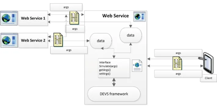
4.2. Identification of Parameters Influence
In order to identify the model parameters that must be chosen with care because of their large impact on model predictions, a simple univariate sensitivity analysis is per-formed to assess how the ASD values are affected by a parameter changes (cf. Figure 6). In this study, between the twelve parameters used in the formulas, three classes of en-vironmental parameters are particularly sensitive to the model.
1. Physical parameters:
The local terrain slope angle (
α
). The fuel depth (e).2. Chemical parameters:
The heat yield of the fuel (∆Hc). The specific heat (Cp).
The moisture content of the dead fuel (m).
3. Meteorological data like the normal wind speed or ambient temperature (Ta). One can note that there is no chemical data available on the net, and all other pa-rameters are not sufficient in temporal and spatial resolution to be used directly in a surface fire spread model. The chosen variable parameters are to the local terrain slope angle, the fuel depth, the normal wind speed and the ambient temperature. All other values are estimated depending on experimental measures or literature researches.
This analysis shows that parameters with significant effects on ASD evaluation are the normal wind speed and the fuel depth. However, local terrain slope but above am-
(a) (b)
[image:15.595.197.552.447.692.2](c) (d)
bient temperature have less influence on ASD and do not produce significant changes on the final results. The results in Figure 6(a) and Figure 6(c) may be surprising, but it can be explained, since the radiation rate directly depends on the fire front length. Wind and slope incline the fire front, thus decreasing the radiation rate perceived by fire fighters. So, it is not necessary, to require a highly accurate estimate on these pa-rameters.
Web Services to determine the local slope and the meteorological data are sufficient to calculate the ASD but there is no service which provides access to fuel depth. So, this value must be given with great precision between zero and two meters, by the user.
4.3. Mapping a DEVS Model to a DEVS Service
To transform our ASD-DEVS models into Web Service, some previous works were used. The proposed application is based on the following technologies: a simulation framework in Ruby and based on the flat DEVS simulator. Our framework is hosted on a server; an interface in Ruby makes a link between the simulator and the data retrieved by the client, and/or other Web Services. This interface allows remote start the simula-tion, and sends the results. The underlying technologies used Internet standards: XML, KML and JSON for data transfer.
REST architecture to drive communications.
Google Map SDK to display on the client, we use the. The steps of this process are:
The Client (tablet or browser) sends data to the server interface.
The interface collects local data. Client data, and other external data by querying other Web Services.
The simulation is performed. The results are sent to the Client.
4.3.1. Underlying Technologies
REST (RE presentational State Transfer) architecture has emerged as a predominant Web Service design model for its simplicity and clarity. So, the Web Service with this architecture is selected. Furthermore, only URIs and HTTP verbs are necessary to ex-pose these methods.
Client/server communications are made through URIs to hand over parameters. Re-sults from server are sent as KML. One can note that KML or Keyhole Markup Lan-guage is an XML notation for expressing geographic annotation and became an inter-national standard of the Open Geospatial Consortium in 2008. The main interest of sending back data as KML format is that the clients don’t have to interpret raw results before drawing them on a map. Moreover this format can be used directly to save the data results in order to use them later.
4.3.2. ASD-DEVS Service
Ori-ented Architectures aims to organize several software components as services providing properties including loose coupling, abstraction and reusability among others.
The solution is composed of several operations, each representing a service: Data Contracts: supplies APIs to access data.
Data: supplies an implementation of Data Contracts APIs (elevation data, tempera-ture and wind speed through external Web Services and ASD from local simulation results).
DEVS Modeling: the modelling abstraction of our original DEVS framework (con-tains ASD models implementations among others).
DEVS Simulation: this layer was part of the original DEVS framework (provides the DEVS simulators).
Services Contracts: represents the API of the proposed service.
Services: implements the Web Service using the API described in Services Contracts. The API of the ASD Web Service is quite simple. It’s composed of one single method available through an HTTP GET request with the following pattern:
/asd/{encoded_polyline}.{format}
The encoded_polyline variable is a string representing a set of latitudes and
longi-tudes encoded following Google’s encoded polyline format (“Google Encoded Poly-line”). It allows to represent several locations concisely. For each of those points, a simulation is launched and a KML string that will contain the polyline passed in argu-ments and a polygon representing the ASD area is built by default. The format parame-ter is optional and can take ISON, XML, or KML value. The first two values return a list of distances in meters for each given location (the raw results). The last value is the de-fault one, which sends back KML as described above. It is chosen to reduce to mini-mum the parameters passed to our Web Service. But, some missing parameters are es-sential to calculate results. It is the raison why it is inevitable to retrieve them from ex-ternal Web Services.
4.3.3. Web Services and Data
The ASD computation needs some parameters that depend on environment data re-lated to a given location. Not all of these parameters can be easily collected. So, a selec-tion of those with a significant influence on the results is done. For each of them, next to launch the simulation, it is proposed to retrieve the information (if available) or cali-brating the value of the parameter from a specific case intituled to the “worst case”. Then, users have to evaluate these different values of this specific case. Seeing that the purpose of the tool is to evaluate the size of a fuelbreak, the hypothesis a critical case is appropriate.
To get by using external Web Services some parameters are managed. The local slope of the spot is evaluated by sampling elevation data around the selected area. Services like (“Google Elevation API”) or (“MapQuest Open Elevation”) can supply such data. Once data are sampled around the location, a gradient descent is applied to obtain the local slope of the terrain (cf. Figure 7).
Figure 7. Result obtained with a Google Map Elevation API query.
tory feature, which accept a date along with latitude and longitude coordinates and which returns a summary of the observed weather at the specified location and date in JSON format.
As shown in Figure 8, the request returns a JSON string that contains weather in-formation for a given area including: maximum, average and minimal values for the wind speed, direction and temperature along with various parameters omitted for this application. Using this data, it can be possible too to evaluate the mean values for a given period can be established (for instance, mean of max temperatures and max wind speed for the last summer).
When, all the parameters cited above are collected, it is possible to launch the simu-lation and send back the results to the client, which can display them on screen.
4.4. Computation of ASD for Various Vegetation Types
This section deals with the computation of Acceptable Safety Distances in which a fire spreads across five different fuels in the Mediterranean area (the intrinsic characteris-tics of each fuel are detailed in (Proterina-C, 2013). Two wind speed values are ran-domly chosen (3 and 5 m∙s−1). Table 5 presents the ASD obtained with the physical
model presented herein.
As the physical model (especially the flame length sub-model) gives a good precision (see the errors given in Table 2, Table 3 and Table 6), it is necessary to have either ac-curate characteristics of the vegetal stratum or a good modeling for an equivalent fuel.
4.5. Displaying
ASD results provided by this Web Service must be useful for firefighters on field when evaluating distances for fuel break. So, the Client must then provide a clear GUI to vi-sualize the terrain and our results. This Client must propose an unobtrusive way to feed input data and a way to retry computations in case of a network failure. In order to fit a such requirement, the Client has been implemented as a mobile application on both iOS and Android platforms and imagined to run primarily on tablets. The user inter-face is essentially composed of:
A sliding panel on the left side providing a section containing a list of previous cached computations and the ability to create a new one.
Figure 8. Result extract of a weather history query.
Table 6. Observed and predicted flame lengths during the Corsican mountain experiment.
Model Flame length (m) NMSE (%) FB (-)
Rate of spread (cm·s−1) 13.74
Observed 2.23
Physical model 2.36 0.35 0.05
Burrows (Burrows, 1994) 1.71 6.90 −0.26
Butler et al. (Butler et al., 2004) 1.09 52.59 −0.68
Byram (Byram, 1959) 1.34 26.14 −0.49
Catchpole et al. (Catchpole et al., 1998) 1.04 59.68 −0.72
Clark (Clark, 1983) 0.33 478.9 −1.47
Fernandes et al. (Fernandes et al., 2009) 1.30 29.22 −0.52 Fernandes et al. (Fernandes et al., 2000) 0.85 98.54 −0.88
Nelson (Nelson Jr., 1980) 0.98 70.60 −0.77
Nelson and Adkins (Nelson Jr. & Adkins, 1986) 1.01 65.83 −0.75 Van Wilgen (van Wilgen et al., 1985) 1.11 50.38 −0.66
Vega et al. (Vega et al., 1998) 1.85 3.46 −0.18
The map has three distinct modes: 1. The normal mode.
2. The user-tracking mode. 3. The drawing mode.
These modes are detailed below:
The normal mode: displays all available data for the current selected computation and allows user interaction to show detailed information.
The user-tracking mode: this Web Service input is basically a set of coordinates. So, as the user location is updated can be spawned to the Web Service and draw a poly-gon that will represent the ASD.
The drawing mode: the user puts a set of locations directly on the terrain and ad-justs each of them.
[image:19.595.196.553.256.516.2]Figure 9. DIMZAL. Display example.
5. Conclusion
This paper presents a multidisciplinary work and argues a software tool (DIMZAL) to compute Acceptable Safety Distance (ASD). This distance was usually set thanks to a general rule-of-thumb: it should be at least 4 times the maximum flame length. This distance is very important because it is used to design fuel breaks. In the proposed ap-proach, to quantify this ASD, a closed physical model is used, including a physical propagation model, a flame length submodel and an analytical model for the computa-tion of ASD. The model is hosted as a web service, and used a simulacomputa-tion framework based on Discrete EVent system Specification formalism (DEVS). In this new work, various results based on the vegetation characterization are presented. Model predic-tions are compared against measured flame length of spreading fires through shrub ve-getation. This work shows that the simplified physical approach presents a main ad-vantage: its capability to be used for all types of fires under a wide range of conditions if fuel models, describing structural types of vegetation, are available. So, this tool can be seen as an alternative operational length flame model, which can be applied to calculate more accurately safety distances and to forecast fuelbreak safety zone sizes at the field scale.
Acknowledgements
The present work was supported in part by the French Ministry of Research, the Corsi-can Region and the CNRS, under Grant CPER 2007-2013. We are thankful to the co-operation of our staff and the team of “Sapeurs Forestiers, Conseilgénéral de la Corse du Sud”. Particularly, we would like to express our gratitude to Mr. Michel Costa and Mr. Gregory Romani of the staff of who helped us to conduct this study despite their busy schedule.
References
Intensity in Predicting Crown Fire Initiation and Crown Scorch Height. International Journal of Wildland Fire, 21, 95-113. https://doi.org/10.1071/WF11001
Andrews, P. L., Heinsch, F. A., & Shelvan, L. (2011). How to Generate and Interpret Fire Charac-teristics Charts for Surface and Crown Fire Behavior.
Balbi, J.-H., Morandini, F., Silvani, X., Filippi, J. B., & Rinieri, F. (2009). A Physical Model for Wildland Fires. Combustion and Flame, 156, 2217-2230.
https://doi.org/10.1016/j.combustflame.2009.07.010
Balbi, J.-H., Rossi, J.-L., Marcelli, T., & Chatelon, F.-J. (2010). Physical Modeling of Surface Fire under Nonparallel Wind and Slope Conditions. Combustion Science and Technology, 182, 922-939. http://www.tandfonline.com/doi/abs/10.1080/00102200903485178
https://doi.org/10.1080/00102200903485178
Balbi, J.-H., Rossi, J.-L., Marcelli, T., & Santoni, P.-A. (2007). A 3D Physical Real-Time Model of Surface Fires Across Fuel Beds. Combustion Science and Technology, 179, 2511-2537. http://www.tandfonline.com/doi/pdf/10.1080/00102200701484449
https://doi.org/10.1080/00102200701484449
Bisgambiglia, P.-A., Filippi, J. B., & Gentili, E. (2006). A Fuzzy Approach of Modeling Evolutio-nary Interfaces Systems. In IEEE (Ed.), 1st international Symposium on Environment Identi-ties and Mediterranean Area (pp. 98-103). New York: IEEE.
Bisgambiglia, P.-A., Franceschini, R., Chatelon, F.-J., Rossi, J.-L., & Bisgambiglia, P. A. (2014). Mobile Application Based on a Physical Model to Calculate Acceptable Safety Distance. In D. X. Viegas (Ed.), 7th International Conference on Forest Fire Research (p. 167). Coimbra: Imprensa da Universidade de Coimbra. https://doi.org/10.14195/978-989-26-0884-6_157 Bisgambiglia, P.-A., Franceschini, R., Chatelon, F.-J., Rossi, J.-L., & Bisgambiglia, P. A. (2013).
Discrete Event Formalism to Calculate Acceptable Safety Distance. In R. Pasupathy, S. H. Kim, A. Tolk, R. Hill, & M. E. Kuhl (Eds.), 2013 Winter Simulation Conference (WSC) (pp. 217-228). New York: IEEE. https://doi.org/10.1109/WSC.2013.6721421
Burrows, J. K. (1994). Experimental Development of a Fire Management Model for Jarrah (Euca-lyptus marginata ex Sm) Forest. Canberra: Australian National University.
Butler, B., & Cohen, J. (1998). Firefighter Safety Zones: A Theoretical Model Based on Radiative Heating. International Journal of Wildland Fire, 8, 73-77. https://doi.org/10.1071/WF9980073 Butler, B. W. (2014). Wildland Firefighter Safety Zones: A Review of Past Science and Summary
of Future Needs. International Journal of Wildland Fire, 23, 295-308. https://doi.org/10.1071/WF13021
Butler, B. W., Finney, M., Andrews, P. L., & Albini, F. (2004). A radiation-Driven Model for Crown Fire Spread. Canadian Journal of Forest Research, 34, 1588-1599.
https://doi.org/10.1139/x04-074
Byram, G. M. (1959). Combustion of Forest Fuels. In K. P. Davis (Ed.), Forest Fire: Control and Use (pp. 61-89). New York: McGraw-Hill.
Catchpole, B. R. A., Choate, J., Fogarty. L. G., Gellie, N., McCarthy, G. J., McCaw, W. R., Mars-den-Smedley, J. B., & Pearce, G. W. L. (1998). Co-Operative Development of Equations for Heathland Fire Behaviour. 3rd International Conference on Forest Fire Research and 14th Fire and Forest Meteorology Conference, 1, 631-645.
Chetehouna, K., Séro-Guillaume, O., Sochet, I., & Degiovanni, A. (2008). On the Experimental Determination of Flame Front Positions and of Propagation Parameters for a Fire. Interna-tional Journal of Thermal Sciences, 47, 1148-1157.
https://doi.org/10.1016/j.ijthermalsci.2007.10.006
Clark, R. G. (1983). Threshold Requirements for Fire Spread in Grassland Fuels. Lubbock, TX: Texas Tech University.
for Assessing Damage Resulting from Marine Spills. Report No. CG-D-38-79, Washington DC. Fernandes, P. M., Botelho, H. S., Rego, F. C., & Loureiro, C. (2009). Empirical Modelling of
Sur-face Fire Behaviour in Maritime Pine Stands. International Journal of Wildland Fire, 18, 698- 710. https://doi.org/10.1071/WF08023
Fernandes, P. M., Catchpole, W. R., & Rego, F. C. (2000). Shrubland Fire Behaviour Modelling with Microplot Data. Canadian Journal of Forest Research-Revue, 30, 889-899.
https://doi.org/10.1139/x00-012
Franceschini, R., & Bisgambiglia, P.-A. (2014). Decentralized Approach for Efficient Simulation of Devs Models. In B. Grabot, B. Vallespir, S. Gomes, A. Bouras, & D. Kiristsis (Eds.), IFIP In-ternational Conference on Advances in Production Management Systems (pp. 336-343). Ber-lin: Springer. https://doi.org/10.1007/978-3-662-44733-8_42
Franceschini, R., Bisgambiglia, P. A., Bisgambiglia, P. A., & Hill, D. R. C. (2014). DEVS-Ruby: A Domain Specific Language for DEVS Modeling and Simulation (WIP). In IEEE Computer Society, Proceedings of the Symposium on Theory of Modeling & Simulation (pp. 393-398). Tampa:IEEE.
Green, L. R., & Schimke, H. E. (1971). Guides for Fuel-Breaks in Sierra Nevada Mixed-Conifer Type.
Harzallah, Y., Michel, V., Liu, Q., & Wainer, G. (2008). Distributed Simulation and Web Map Mash-Up for Forest Fire Spread. In IEEE Computer Society, Proceedings of the 2008 IEEE Congress on Services (pp. 176-183).New York: IEEE.
https://doi.org/10.1109/SERVICES-1.2008.74
Higgins, S. I., Bond, W. J., Trollope, W. S. W., & Williams, R. J. (2008). Physically Motivated Empirical Models for the Spread and Intensity of Grass Fires. International Journal of Wild-land Fire, 17, 595-601. https://doi.org/10.1071/WF06037
JAI (2009). Camera Jai AD-o8oGE. http://www.graftek.com/pdf/Brochures/JAI/AD-080GE.pdf Kim, K. H., & Kang, W. S. (2005). A Web Services-Based Distributed Simulation Architecture for
Hierarchical DEVS Models. In T. G. Kim (Ed.), 13th International Conference on AI, Simu- lation, Planning in High Autonomy Systems (pp. 370-379). Berlin: Springer.
https://doi.org/10.1007/978-3-540-30583-5_40
Marcelli, T., Balbi, J.-H., Moretti, B., Rossi, J.-L., & Chatelon, F.-J. (2011). Flame Height Model of a Spreading Surface Fire. In MCS7, 7th Mediterranean Combustion Symposium (pp. 11-15). Cagliari: Combustion Institute.
Mittal, S., Risco, J. L., & Zeigler, B. P. (2007). DEVS-Based Simulation Web Services for Net-Centric T&E. 2007 Summer Simulation Multiconference, 1, 357-366.
http://www.scopus.com/inward/record.url?eid=2-s2.0-84870159320&partnerID=40&md5=464 b50db9dda751a6c00383901945b5c
Morandini, F., Silvani, X., Rossi, L., Santoni, P. A., Simeoni, A., Balbi, J. H., Louis Rossi, J., & Marcelli, T. (2006). Fire Spread Experiment across Mediterranean Shrub: Influence of Wind on Flame Front Properties. Fire Safety Journal, 41, 229-235.
https://doi.org/10.1016/j.firesaf.2006.01.006
Morvan, D., Tauleigne, V., & Dupuy, J.-L. (2002). Flame Geometry and Surface to Crown Fire Transition during the Propagation of a Line Fire through a Mediterranean Shrub. In D. X. Viegas (Ed.), 4th International Conference on Forest Fire Research (10 p). Rotterdam: Mill Press.
Muzy, A., Innocenti, E., Aiello, A., Santucci, J.-F., & Wainer, G. (2002). Cell-DEVS Quantization Techniques in a Fire Spreading Application. 2002 Winter Simulation Conference, 1, 542-549. https://doi.org/10.1109/WSC.2002.1172929
1010-1022). New York: IEEE. https://doi.org/10.1109/WSC.2011.6147825
Nelson Jr., R. M. (1980). Flame Characteristics for Fires in Southern Fuels. USDA Forest Service, General Research Paper SE-205, Asheville, NC: Southeast Forest Experimental Station. Nelson Jr., R. M., & Adkins, C W. (1986). Flame Characteristics of Wind-Driven Surface Fires.
Canadian Journal of Forest Research, 16, 1293-1300. https://doi.org/10.1139/x86-229 Proterina, C. (2013). PO Italia-Francia “Maritimo” Rapport PR3.3.3.
Raj, P. K. (2008). A Review of the Criteria for People Exposure to Radiant Heat Flux from Fires. Journal of Hazardous Materials, 159, 61-71. https://doi.org/10.1016/j.jhazmat.2007.09.120 Rossi, J. L., Simeoni, A., Moretti, B., & Leroy-Cancellieri, V. (2011). An Analytical Model Based
on Radiative Heating for the Determination of Safety Distances for Wildland Fires. Fire Safety Journal, 46, 520-527. https://doi.org/10.1016/j.firesaf.2011.07.007
Rossi, L., Molinier, T., Akhloufi, M., Pieri, A., & Tison, Y. (2013). Advanced Stereovision System for Fire Spreading Study. Fire Safety Journal, 60, 64-72
https://doi.org/10.1016/j.firesaf.2012.10.015
Rossi, L., Toulouse, T., Cancellieri, D., Rossi, J.-L., Morandini, F., & Akhloufi, M. (2014). Utilisa-tion de la stéréovision visible et proche infrarouge pour la mesure de données expérimentales dans le cadre d’une recherché pluridisciplinaire sur les feux de forêt. Journal National de la Recherche en IUT, 33-44
Santoni, P. A., Simeoni, A., Rossi, J. L., Bosseur, F., Morandini, F., Silvani, X., Balbi, J. H., Cancel-lieri, D., & Rossi, L. (2006). Instrumentation of Wildland Fire: Characterisation of a Fire Spreading through a Mediterranean Shrub. Fire Safety Journal, 41, 171-184.
https://doi.org/10.1016/j.firesaf.2005.11.010
Seo, C., & Ziegler, B. P. (2012). Simulation Model Standardization through Web Services: Inte-roperation and Federation on the DEVS/SOA Platform. In IEEE Computer Society, Pro- ceed-ings of the 2012 Symposium on Theory of Modeling and Simulation (pp. 46.1-46.8). Orlando: IEEE.
Van Wilgen, B. W., Le Maitre, D. C., & Kruger, F. J. (1985). Fire Behaviour in South African Fynbos (Macchia) Vegetation and Predictions from Rothermel’s Fire Model. Journal of Ap-plied Ecology, 22, 207-216. https://doi.org/10.2307/2403338
Vega, J. A., Cuinas, P., Fonturbel, T., Perez-Gorostiaga, P., & Fernandez, C. (1998). Predicting Fire Behavior in Galician (NW Spain) Shrubland Fuel Complexes. Proceedings of 3rd Interna-tional Conference on Forest Fire Research and 14th Conference on Fire and Forest Meteorol-ogy, 2, 713-728.
Zacharewicz, G., Hamri, M. E.-A., Frydman, C. S., & Giambiasi, N. (2010). A Generalized Dis-crete Event System (G-DEVS) Flattened Simulation Structure: Application to High-Level Ar-chitecture (HLA) Compliant Simulation of Workflow. Simulation, 86, 181-197.
https://doi.org/10.1177/0037549709359357
Zárate, L., Arnaldos, J., & Casal, J. (2008). Establishing Safety Distances for Wildland Fires. Fire Safety Journal, 43, 565-575. https://doi.org/10.1016/j.firesaf.2008.01.001
Submit or recommend next manuscript to SCIRP and we will provide best service for you:
Accepting pre-submission inquiries through Email, Facebook, LinkedIn, Twitter, etc. A wide selection of journals (inclusive of 9 subjects, more than 200 journals)
Providing 24-hour high-quality service User-friendly online submission system Fair and swift peer-review system
Efficient typesetting and proofreading procedure
Display of the result of downloads and visits, as well as the number of cited articles Maximum dissemination of your research work