ISSN Online: 2327-4344 ISSN Print: 2327-4336
Processing and Unification of Environmental
Noise Data from Road Traffic with Spatial
Dimension Collected through Mobile Phones
Petr Duda
Laboratory on Geoinformatics and Cartography, Masaryk University, Brno, Czech Republic
Abstract
Noise measurement using mobile phones is now developed very well. While there are some good applications for the measurement of noise from road traffic, thus on processing of measured data is only paid a very little attention. The data, however, are burdened by specific errors and for further work with them it is necessary to adjust and determine their uncertainty. One of the big-gest problems is inaccuracy in position versus the noise source and the short-est length of measurement that can be regarded as representative. Imprecision in terms of location can be determined by calculating the variance of possible distance from the noise source, which for measurement of traffic noise re-quires a map-matching data points both transverse to the street (sidewalk) network and in the longwise direction. During typical urban measurements, this error can even reach 7 - 10 dB. Three basic types of algorithms for the calculation of uncertainty and positional correction based on the type of input and output data (raster, vector, vector-oriented) were tested. Uncertainty in the variability of the measurement data is necessary to determine from the number of passing vehicles per time unit. The presented solutions are imple-mented in the Mobile Noise system.
Keywords
Measurement Uncertainty, Environmental Noise, Mobile Phone, Citizen Science, Noise Mapping
1. Crowdsourcing of Environmental Noise Measurement
Currently, there is a massive expansion of a new phenomenon: use of mobile How to cite this paper: Duda, P. (2016)
Processing and Unification of Environmen-tal Noise Data from Road Traffic with Spa-tial Dimension Collected through Mobile Phones. Journal of Geoscience and Envi-ronment Protection, 4, 1-26.
http://dx.doi.org/10.4236/gep.2016.413001
Received: July 21, 2016 Accepted: December 24, 2016 Published: December 27, 2016
Copyright © 2016 by author and Scientific Research Publishing Inc. This work is licensed under the Creative Commons Attribution International License (CC BY 4.0).
http://creativecommons.org/licenses/by/4.0/
phones for data collection and then voluntary collection and processing of the data using a variety of social networks. This concept can be applied among oth-ers, also to the problem of environmental noise pollution. Although it has a number of limitations, as demonstrated by first studies (e.g. [1] [2]), it may suc-cessfully act as an appropriate complementary tool for monitoring and assess-ment of the damage caused by excessive noise.
Over the past 10 years, several projects in the field of community noise map-ping have been created. These projects are primarily trying to introduce noise mapping technology using mobile phones and processing of data acquired by this way. Albeit, relatively large amount of data have been collected by these stu-dies. Further use of these data still remains a big question. These studies were primarily aimed to test the concept of noise data crowdsourcing, while they did not develop issues of their further processing and use. This kind of data, if they are published at all, most often rely on the fact that they will be used in their raw form. This approach significantly reduces usefulness of the data for further analysis and evaluation of noise situation. This article primarily focuses on post processing of the noise data on example of ground transportation noise data from the point of view of the uncertainties in the positioning and in terms of changes in land transport operations during daytime.
1.1. Smartphone Applications for Crowdsourced Noise Measurement
The work of Santini et al. [3] was one of the first to use mobile phones to meas-ure environmental noise. Authors particularly examine technical problems that affect the design and implementation of systems which use mobile phones to as-sess noise pollution. This paper is not yet focused on the development of the en-tire system and noise maps cannot be created from presented incomplete and random sampling. Later, e.g. at work [4] authors presents full system for noise mapping, but this system lacks A weighting filtering as input procedure for ob-tain the equivalent noise levels, so it is not possible to compare outputs with standard noise maps.
The most important systems able to map noise using smartphones as sensors, however, are these:
• NoiseSpy [5]—This application is one of the first which allows collection of
spectrum. Data are not adjusted in any way. Application and data were never released to the public.
• NoiseDroid [6]—Application allowing collection of data on noise using
mo-bile phones with the Android operating system. It supports manual, auto-matic, event or series measurements and visualizes all the collected mea-surements as a table or a map. Data can be viewed and filtered by various criteria. Users can export measurement results to the Open Noise Map web portal and they are also able to import measurements from this community server. Source code is available, but the application itself is no longer being developed and maintained. There is, or should be, an interface for Google Maps, Open Street Maps, Bing Maps and Ovi Maps. Map visualizes the noise level by so-called heat map, data are clustered using the DBSCAN algorithm
[7]. Again, there is complete lack of any further data processing.
• NoiseMap [8]—This is a noise map from mobile phones sensors in history
and in real time. It is a part of the project for visualization of data from vari-ous sensors using da_sense.de software. This map is visualized using a hex-agonal grid, where color scale shows the noise level. A coupled mobile appli-cation for data measurement called with same name is presenting also a fre-quency calibration and incentive mechanisms (gaining points for success measurements) and is downloadable for Android platforms. The source code is currently not accessible.
• AirCasting [9]—Initiative of a non-governmental organization based in New
York [10]. They, in cooperation with a Polish subcontractor, developed an application for Android, which allows to collect data on noise. Web portal allows to visualize also a large number of other parameters from other types of sensors (dust, moisture levels of CO, CO2, etc.). Wherein there is no sensor
classification, it is very difficult to search, view and process appropriate data type. Users can annotate data by text, signs and photographs. Both the mo-bile application and the Web platform are open source. In the momo-bile appli-cation, users can calibrate the input using a trim application method. On the web portal, data are dynamically clustered into a square grid and using this grid an average values are calculated for a every grid cell with measurements. However, this application lacks measuring accuracy specification.
• WideNoise [11]—An application developed for mobile phones with
website, where they are displayed on a map. In 2011, based on the project Every Aware [11], an updated version 3.0 was processed, where also annota-tions are available. Source code of WideNoise v3.0 for iOS and Android is available under open source license. WideNoise uses linear interpolation to compensate microphone sensitivity etc. It is not possible to calibrate the ap-plication for different types of devices.
• Ear-Phone [13]—This project presents a general solution for monitoring
en-vironmental noise using mobile phones. The main task of this system is find how to solve the fundamental problem to get noise maps from incomplete and random samples obtained by crowdsourcing data collection. Different interpolation and classification methods are used for achieving this target. Ear-Phone, which is implemented on the Nokia N95 and N97, HP iPAQ and HTC One, also addresses the question of the measurement precision and da-ta of noise pollution collection on the mobile device. One of the biggest problems using smart phones as sensors is that the results of the sensor mea-surements may vary depending on the orientation of the phone and the user's context (for example, if the user carries the phone in a bag or hold it in your hand). To solve this problem, Ear-Phone introduces detection of device rela-tive position context, and application there under automatically determines whether a measurement makes sense or not. Ear-Phone also implements the so-called calibration in situ, which means a simple calibration which can be performed by only the general public. Huge disadvantage of this system is its closeness and inaccessibility.
• Bike Net [14]—An experimental mobile sensor system designed for cyclists.
It uses smart phones equipped with GPS, which are connected to additional external sensors. The system records the traveled distance, speed, burned calories, terrain roughness, CO2 levels and noise levels in the area. This data
could be stored on a simple web portal called Bike View [15], which allowed to visualize routes and sensor measurements on the map. Currently the ap-plication is out of operation.
• Noise Tube [16]—This is currently the most advanced open and accessible
o It does not allow universal machine processing and accessing to noise data, as
the proposed application interface is local and does not reflect the sensory standards and does not allow a broader machine processing of given tags, these characters are treated as a cloud data.
o Noise situation is mapped to the street network on the server, but this
map-ping does not reflect possible errors in the position measurement.
o Application has options to categorize the different models of mobile phones
into the quality classes, but does not evaluate the quality of individual mea-surements. It does not take into account the spatial or temporal circums-tances (such as adjacency of measurement points, time of day, etc.).
1.2. Character of the Noise Data from Smartphone Crowdsourcing Applications
The main feature of all these systems here is focus on the sensor platform-a mo-bile phone, and on the ways in which data may be collected, how the phone can be calibrated and, where appropriate, to eliminate the worst interference when measuring. This approach is logical because without quality and reliable sensor it is not possible to obtain high-quality sensor data. The experience gained from these projects can be summarized as follows:
• Mobile phone platform as the sensor platform is suitable for measuring noise under these conditions and restrictions:
o Mobile phone is a multifunction device; it is necessary to monitor its use.
o Mobile phone must have an Internet connection.
o Calibration of mobile phones is a very sophisticated issue, but automatic
ca-libration is a solvable problem.
o One of the biggest problems is battery life, which is consumed mainly by
GNSS sensor and by data transmissions.
• Noise data obtained by measuring using a mobile phone has the following
limitations:
o They are incomplete. There must be an algorithm for its adjustment and
completion, or at least to determining the degree of completeness.
o They are spatially inaccurate, so must be spatially refined.
o They are focused on serial measuring.
o They must be anonymized.
However, the main feature of such works is the pursuit of technical-engi- neering view on measuring, which causes a certain distance from other segments of noise data processing. While most of the problems associated with mobile phones’ measuring is at least partially solved, given works are only marginally engaged in further processing of the measured data, which primarily means:
• Quantifying and eliminating uncertainties associated with position errors of small and cheap GNSS sensors which are a usual part of today’s smartphones,
• Quantification and classification of data in space and time, including in
o Detection of a noise source based on the closeness.
o Quantifying the impact of noise on the surroundings.
o Detection of spatial and temporal patterns, classification and analysis of such
patterns.
• Visualization noise levels and their uncertainties.
o Setting basic rules and procedures, a survey of algorithms.
o Interpretation of measured values by users.
• Openness of systems for further use by other systems and surveying of open
standards for the transmission of sensory information, both in the raw and in the processed form.
This last point is particularly important because if the systems declare neces-sary openness both in the data and in the procedures, it is more than appropriate to exploit the possibilities of open data formats. Although these systems often have their own open application interface, the form of integration between par-ticular noise measurement systems was not sufficiently explored.
2. Specifics of Noise Measurements Using a Mobile Phone
The main difference of noise mapping using mobile phones from traditional mapping is the approach to classification of noise sources. Current applications, which are using mobile phones for noise measurements utilize person-centra- lized approach in which the mobile phone is used as a noise-dose meter, which indicates the overall affection rate by noise for one particular person (an equiva-lent of radiation dosimeters). Noise level along with time and eventually position is recorded every second (which corresponds to the “slow” measurement stan-dard for stanstan-dard noise meters).
This approach is, in comparison with conventional mapping of the spatial distribution of noise, considerably easier. There are primarily not distinguished individual sources of noise, including noise, which is created by user. Informa-tion about the posiInforma-tion of measurement is secondary, may not even be filled, and is used more for orientative purposes. For information purport, such work with a location is quite sufficient, but in case of study of the spatial distribution of noise there should be a somewhat more sensitive approach.
Despite these shortcomings, it can be said that even the dosimetry data, if col-lected sufficiently accurately, can be used for compiling maps of spatial distribu-tion of noise or even be combined with data from convendistribu-tional measurements. This approach is also used in a number of mobile applications that allow to vi-sualize the measurements in the map, assuming that measurements are per-formed while walking.
2.1. The Issue: Uncertainties of Measurements of Noise by Mobile Phones
quantities of individual sources of noise measurement errors. Standards ISO 3745 [18] and ISO 1996-2 [19] identify some of the most important sources of error and their overall contribution can be written as follows:
,true ,
Aeq Aeq m slm sou met loc res
L =L +δ +δ +δ +δ +δ +ε (1)
where LAeq, true is true equivalent sound pressure level adjusted by weighting
fil-ter A, LAeq, m sound pressure level measured by noise meter and adjusted by the
weighting filter A, δslm is an error in the measurement chain (sound level meter
in the simplest case), δsou is an error caused by the difference from ideal
operat-ing conditions of noise source, δmet is the error caused by meteorological
condi-tions different from ideal, δloc is a positional sensor error, δres is an error on
resi-dual noise level and ε resiresi-dual error. δsou + δmet are for static measurements often
obtained directly by measuring in the point of interest, but when measuring us-ing mobile phones on the move, only meteorological data available often are, and these only from the remote weather stations.
Uncertainty of each measurement can then be expressed by the error propa-gation law as:
(
)
(
)
22 2 2 2 2 2
, sou
Aeq m slm met loc res res
u L =u +u +u +u + c ⋅u +ε (2)
where cres is a sensitive coefficient for residual coefficient (other sensitive
coeffi-cients are equal to 1.0).
Table 1 of ISO 1996-2 [18] contains an overview of the measurement uncer-tainty for the A-equivalent noise level. Higher uncertainties are to be expected on maximum levels, frequency band levels and levels of tonal components in noise.
[image:7.595.211.539.522.707.2]The article focuses primarily on uncertainty of localization, but preliminary is necessary for clarity, at least briefly discuss the accuracy of the actual measured noise level in the case of mobile phone measurement.
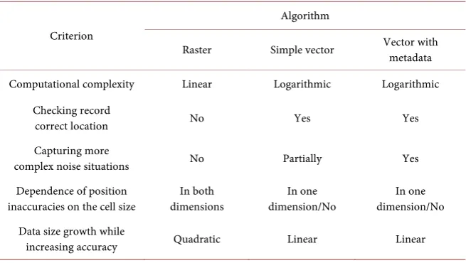
Table 1. Comparison of methods for determining spatial measurement noise uncertainty.
Criterion
Algorithm
Raster Simple vector Vector with metadata
Computational complexity Linear Logarithmic Logarithmic
Checking record
correct location No Yes Yes
Capturing more
complex noise situations No Partially Yes
Dependence of position inaccuracies on the cell size
In both dimensions
In one dimension/No
In one dimension/No Data size growth while
2.2. Accuracy of Mobile Phones’ Microphones
It is obvious that the accuracy of mobile phone sensors (microphones) is lower than the accuracy of certified noise meters. This drawback, however, is possible to almost completely eliminate by using accurate calibration, at least in case of noise measurements of surface transport.
The laboratory experiments have shown that sensors built in mobile phones have a surprisingly high accuracy when measuring the acoustic noise levels, which is, while applying correct calibration and measurement interval 1 second, in the range of about 35 - 110 dB gets below the value of ±1 dB [20] [21].
Field tests in synergy measurement with the noise meter of Class 2 according to IEC 61672-1 [22] shown that during normal measurement of urban noise sit-uation also deviation of ±1 dB from the values measured by given noise meter
[20] [21]. For the actual level meters of Class 2 was detected uncertainty of ±2 dB [23]. For accurate practical results preliminary synergistic measurement with certified Class I noise meter was performed wherein deviation does not exceed ±2 dB in any of the cases of non-impulse noise.
The disadvantage of microphones from mobile phones is mainly a lower dy-namic of sensor and the resulting slower response, therefore these sensors are not suitable for measurement of impulsive noise, but for measuring of most cas-es of noise from ground traffic and many kinds of neighborhood noise are suffi-cient.
Uncertainty of microphones precision varies from type by type and also piece by piece. Issues of calibration of individual phones are quite extensive and are outside of this text scope. Basic information can be obtained e.g. in [24].
2.3. Positional Accuracy When Measuring Noise
Mobile phones, especially in urban areas, suffer from higher inaccuracies in po-sitioning. This is essentially a problem of GPS device, which may receive re-flected radio signal instead of direct, thereby calculate erroneous distance be-tween GPS transmitter and receiver, which consequently leads to erroneous po-sitioning. The inaccuracy may be in the order of first units to tens of meters. In some case the location of the resulting data points is automatically adjust5d, for instance, when measured on the street network, but the location data will indi-cate the location inside buildings. Such results, however, have limited relevance.
important role. As the practice shows accuracy of GPS (and assisted GPS) re-ceivers in mobile phones varies widely and common deviations reach values from 3 to 10 m, and in some cases even to 40 m [25].
In the case when an accurate knowledge of the position of a noise sensor is not guaranteed (at least in the order of decimeters), it is not possible to determine noise value at the place of its origin and thus obtain information about the noise situation in the area. Values are only valid for the place of measurement, which is itself known with considerable uncertainty.
Maximum uncertainty of noise level in dB increases with uncertainty of the distance, in case of a point source of noise radiating in all directions, according to noise level equation:
(
)
(
2 2)
0 10 4π
L= log P r −r (3)
where P stands for power of sound waves at the source, r is the actual distance from measurement point to the noise source and r0 represents indicated (e.g.
measured using GNSS) distance from measurement point to the noise source. If the noise source is a line, is in case of assignment of measurement point to the correct line segment, where is the impact from another segment of the line lead-ing in different direction negligible, maximum uncertainty of the noise level can be obtained in dB as:
(
)
(
0)
10 2π
L= log P r−r (4)
Because we do not know power of sound waves at the source, to determine the uncertainty of the level of noise at a certain probability level is necessary to de-termine the most probable deviation from the measured noise level. The highest positive value of uncertainty may be, for a point source, determined by the equa-tion:
max – L r s
u L L
+ = (5)
where Lr is the measured noise level at a distance r from the noise source, Lsmax
represents noise level at a distance r from the source of the noise, but if the measured noise level Lr would apply to point at the distance r + e, where e is the
uncertainty value of position in given length rate (e.g. in meters), therefore, for the point furthest from the noise source at given confidence level.
The highest negative value of uncertainty according to equation:
–uL =Lr–Lsmin (6)
where Lr represents the measured noise level at a distance r from the noise
source, Lsmin represents noise level at a distance r from the source of the noise,
but if the measured noise level Lr would apply to point at a distance e, where e is
the uncertainty of value position in the given length rate, i.e. for the point closest to the source of the noise on a given confidence level.
Spatial error of 5 m from a point source of noise that may indicate faulty as-signment noise level to even 15 dB, from a line source (which is for example a road with regular traffic) to about +6 and −10 dB.
Problem grows even more, if users measure the noise when walking, which is currently among the most anticipated applications of crowdsourcing method of measurement. Some of the services used (e.g. Noise Tube) are solving these in-accuracies by assign recorded noise value points to the appropriate points on the street nearest from the recorded position [26]. Such an assignment itself is insuf-ficient, there should still retain significant positional deviations. It is also appro-priate to supplement recorded values user data (user himself specifies the rela-tive position, such as street name, closest house number and the estimate of dis-tance from it, etc.).
The error in this field can then grow even more if insufficiently rigorous pro-cedures and tools to evaluate the noise are utilized. The most common proce-dure for the aggregation of measured values is a regular square grid. Due to GNSS receiver inaccuracies, the most appropriate size of the edges of the square grid cell is considered to be about 20 m so that the value with the highest proba-bility will be actually incorporated into the correct square. But for the calculation of noise in the vicinity of the noise source is required spacing between the calcu-lation points up to 10 m [27]. Therefore, the position of the individual mea-surements must be adjusted.
2.4. Operating Conditions of Noise Source
Operating conditions of noise sources often varies throughout the day. For ex-ample, when measuring the noise on the road network, it is necessary to take into account the current time due to rush hours, all in terms of the day and the week, month and year. Depending on these conditions, a variety of noise de-scriptors that describe the situation was introduced. Among the most commonly used descriptors include:
• Sound pressure level (L) [dB]—may be weighted (e.g. by using the weighting
filter A or C).
• Statistical noise level (Ln)—noise level exceeded for n percent of the
meas-ured interval. (Indicators L1, L10, L50, L90 and L99 are used for a rough estimate
of the maximum noise levels, noise, median and background noise.)
• The equivalent continuous noise level (Leq, TL)—Theoretical noise level, which
describes the noise that varies considerably during the timed interval. If the input value is weighted according to the acoustic weighting filter A, LAeq, T. • The level Lden (day-evening-night)—an indicator of the overall noise.
• Level Lday (day)—indicator for interference-day period, defined as the
weighted (by using the weighting filter A) long-term average sound level ac-cording to ISO 1996-2 [19] designed for any day of the year.
as the weighted long-term average sound level, fixed for all the evening pe-riods of the year.
• The level Lnight (night)—an indicator for disturbances during sleep, defined as
the longer-weighted average sound level, set for any night of the year. From the perspective of crowdsourcing noise measurement is usually suffi-cient just to record the precise time of measurement, in order to correctly assign given records. The actual uncertainties can then be calculated according to eva-luated descriptor.
A much larger problem is the insufficient length of measurements. None of the above mentioned systems does not answer the question whether processed data are sufficiently representative for an objective assessment of noise levels at the site. The criterion of representativeness deals to the character of the behavior of the noise source.
2.5. Weather Influence onto Measurements
Quite a considerable influence on the measured noise level has the weather. There are issues on precipitation (rain drumming up around the sensor), on thunder and especially on the wind, which can greatly affect measured values. Professional sound level meters often use so-called wind guard and, when out-door, also temperature, humidity and wind speed are measured in addition to the noise level.
In the case of mobile phones, compliance with such requirements is relatively complicated, so it is necessary to rely on the expertise of users, and also increase the potential uncertainty of measurement in the case of higher wind speeds or gusts recorded in the nearest available meteorological stations, then might be necessary to excrete such a wide range of measurements, which limits noise measurement capabilities, especially in variable weather. Also there is a possibil-ity of noise frequency analysis that could eventually detect wind gusts.
2.6. Influence of Residual Noise
Residual noise during measurement using mobile phones represents mainly a noise that is emitting by the user alone. It can be both noise caused by walking or biking, and above all the noise from the speaking or operating the phone. In the case that we tolerate the user to move during measuring, there should be no other option than to accept the fact that we can then evaluate the noise up from a certain level, which is about 10 dB higher than the noise caused by walking or driving. Noise level of walk with soft soles on hard subsoil reaches (from our experience) values 30 - 40 dB, in the case of heels or walking on gravel may reach up to 70 dB. It is therefore necessary to exclude or mark such measurements properly [28].
the occasional conversation of pedestrians around should significantly disrupt collected data. In this case it is appropriate either interrupt measurement or rely on the frequency analysis, which allows to detect human conversation and then the measurement is automatically discarded. If the data on the frequency distri-bution are not transmitted to the post processing, it is necessary to carry out these detections and adjustments in the mobile phone, which is very computa-tionally expensive [29] [30] and is typically not performed.
2.7. Summary
There are numerous negative impacts on noise measurements using a mobile phone. Aside from incorrect device operation, it is mainly the effect of mea-surement chain: quality of microphone calibration, processing of noise signal and influence of residual noise from other sources. These areas are dependent upon the input settings or direct measurement circumstances. Their modifica-tion on subsequent processing is very problematic. Quantifying of uncertainty on these effects is directly dependent on knowledge of the whole system.
Additional uncertainties arise from the spatial accuracy, from weather situa-tion and from operating condisitua-tions of the noise source. In crowdsourcing, vir-tually no attention is paid to these uncertainties. But they can be quantified and modified during post-processing. But, on the contrary, during measurement they can be evaluated only by greatly increased effort. Using the following tech-niques and procedures, it is possible to generate a standardized data set which uncertainties are sufficiently reliably quantified and which can thus enter into the subsequent analysis.
3. Processing of Positional Errors of Environmental
Noise Data from Surface Transport Collected through
Mobile Phones
Position of measurements during crowdsourced measurement of traffic noise is necessary to bind primarily to the noise source. This is, from the perspective of surface transport measurement, a track line (e.g. road, rail). Taking i.e. into ac-count the normal noise level emitted by an average passenger car during conti-nuous ride at speed of 50 km/h on normal asphalt surface, when an error 5 m occurs in the position measuring, the measurement error can reach 6 - 10 dB.
[26] Data obtained with this error are therefore highly approximate and may not be used in essentially any more detailed analysis.
However, the position of the measured data can be evaluated such as to make clear what the position error and the value of its contribution is. Then we can evaluate the uncertainty of measurement in dB or fix the position (if possible).
3.1. Aspects of Evaluation of Positional Errors in the Raster Grid
the grid to which both measured values and values of positional uncertainty are aggregated. Data can be clustered into grids based on their recorded position and positional uncertainty both on the basis of estimated spatial error provided by GNSS receiver. However, these data are often not available or the spatial error estimate is unreliable. This applies especially to the urban environment, which is suffering from so-called Street canyon effect, and also in heavier forests where GNSS coverage is usually quite random.
For more reliable determination of uncertainties is thus appropriate to use data, which already have sufficient accuracy—on the one hand for the position-ing of the source—and if possible, especially the estimated position or trajectory, on which the user is moving. For evaluation of noise from land transport this today in practice means the use of spatial databases (maps) of the road network. These databases itself may not suffer from too high positional inaccuracies and must be as complete as possible.
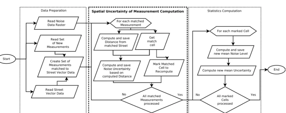
3.2. Algorithm for Evaluation of Positional Errors in the Raster Data Grid with Street Data
Street data are nowadays usually stored in vector databases. For ease of cluster analysis, it is therefore necessary to convert them into raster grid. Thereafter, on the basis of the location attribute, each value of the noise level of the raster cell is averaged and stored in a square raster. In a similar manner is calculated the av-erage deviation of the position of the measuring points from the noise source (so the street, represented by the raster cell or as a direct line string). The result can be easily visualized and further clustered. Overall scheme is depicted on Figure 1.
Between the main features of this algorithm belongs:
[image:13.595.64.539.495.683.2]• High speed of processing and visualization. • Simplicity of implementation.
• It can be, due to the shape of the Earth, applied only locally, so it is important
to determine the area to which it will apply.
• It can’t capture more complex noise situations, whether in horizontal (noise
barriers, intersection, multi-lane roads, etc.) and vertical orientation (espe-cially bridges).
• Assigning a value to the noise source is limited by the size of the aggregating
cell and is heavily dependent on randomness of its position.
• It is not detected whether values are assigned to the correct cells.
• Accuracy of determined uncertainties as well as transitions of noise levels is
highly dependent on cell size. In the case of small cells in a large area is the grow of the volume of needed data and the processing speed inversely pro-portional to the area of the cell.
Despite these disadvantages, the raster method is used for processing and vi-sualization of noise in almost all projects, including those mentioned in Chap-tion 1.1. Most of them do not even take into account the street network yet.
It should also be pointed out that, when assessing the noise situation on land transport using square grid, the shape of the road network plays an important role. In the case that streets are mutually perpendicular, a square grid with the cells oriented in the same direction with the street network allows sufficiently precise and unambiguous assignment of points of the road network to the raster. However, if streets diverge, this situation is much more complicated. Theoreti-cally, it is possible to use other types of raster (triangular, hexagonal, see e.g. Noise Map [7]), but work with these types of raster is much more complex and many advantages of the raster approach is thus considerably reduced.
3.3. Aspects of the Evaluation of Positional Errors in the Vector Model
Vector model allows to evaluate the positional error in with several orders high-er accuracy compared to rasthigh-er model. This in turn allows to map noise sources’ and measurement points’ relative position more accurately. The result could ideally serve to recover the value of sound power of noise sources on sufficient precision. At least, these data can then be used to assess the overall noise situa-tion. However, evaluation of noise levels in the vector model requires much more challenging data preparation. Also calculation itself is also much more complex and takes incomparably longer. But, according to the development of computer technology in recent years, these restrictions cease to be serious. Posi-tional error in the vector model can be determined as the distance to the nearest point on the line of the interpolated position along places designated as vertexes (designated by a user, or a specialized algorithm).
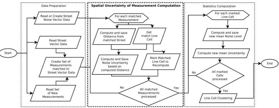
3.4. Simple Algorithm for Evaluation of Positional Errors in Vector Model with Street Data
called line chains (line strings), which in fact are strings of point coordinates. However, from the perspective of assigning noise levels to the streets, repre- sented by the lines, is assumed that the value of both noise levels and the uncer-tainty value will be assigned to a specific section of the line, where the noise situ-ation is practically homogeneous.
In order to determine which part of the line noise is homogeneous, there is hardly an alternative to a regular line divided into segments, where the noise situation will be assessed separately. The size of individual calculation segments can be adjusted according to the required accuracy in terms of noise measure-ments by mobile phones, but can be based on the values specified in chapter 2.3. We can say, that the basic segment length should vary in the values of about 10 - 20 m, because shorter segments already does not provide any substantial in-crease in accuracy. The depiction of this algorithm is on Figure 2.
The algorithm itself is divided into several phases, which take place separately. Firstly, it is necessary to determine the position of each segment in the street network and then is possible to aggregate measured values and their uncertain-ties. Subsequently aggregation of segments with similar data may occur, which saves data space and time for further processing and visualization. The main features of this algorithm are:
• Larger memory and performance requirements. It is appropriate to process
areas sequentially.
• Rather more complex implementation.
• In case of suitably chosen coordinate system, the possibility of a global and
seamless processing enables fully automated handling without human inter-vention.
• Is able to partially capture a more complex noise situation in terms of
[image:15.595.61.539.501.686.2]vertic-al, but still just with limits (such as bridges) and partly also horizontal com-plex situations (e.g. noise barriers, intersection). But it can’t quite adequately
assess the situation in cases of asymmetrical noise situations, more lanes or composition of multiple noise sources (e.g. tramway strip between road lanes).
• Assigning a value to the noise source or noise emission levels on the street is
limited by the size of the aggregate cell only in the longwise direction. It is no longer entirely dependent on a random location of cell boundaries.
• There is a check of the correct assignment of measured value to the source,
because the values are assigned sequentially based on prior knowledge about the direction of monitoring of a series of measurements.
• Accuracy of perceived uncertainties as well as transitions of levels depends
on the cell size and density of the road network, in the case of small cell on a large area is growth in the volume of the necessary data as well as processing speed inversely proportional to the length of a side of the cell.
Noise evaluation using this algorithm also brings the need to address issues which were not necessary to be addressed in the evaluation of noise using raster network, because of its lower spatial accuracy. In case of noise data obtained by pedestrians using mobile phones there is issue on the position of the measure-ment points on the given street cross-sectional profile. Knowledge of the situa-tion in street’s cross secsitua-tion allows accurate determinasitua-tion of uncertainty. For this processing method, it is necessary to obtain additional data from the user.
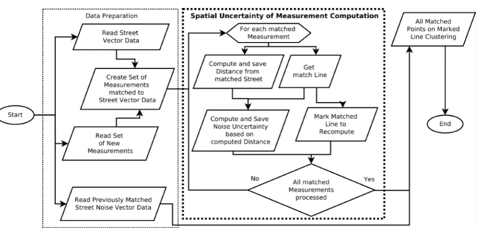
3.5. Algorithm for Evaluation of Positional Errors in the Vector Model with Street Data and Data about the Relative Position and User Movement
As should be obvious from everyday experience for all of us, there are a huge va-riety of street cross-sections, but most vector street network databases represent the street only as a simple line. But if the data about the width of the streets or sidewalks position is available, is possible to determine the distance from the source of pedestrian traffic noise more precisely. And even in the event that such information is not available, it is advisable to remember the information on which side of the street the user is measuring, because from these data is possible to detect any asymmetry of the noise situation later, which may substantially re-fine the further processing and interpretation of noise data. The algorithm scheme is on Figure 3.
Figure 3. Determining spatial uncertainty for noise measurements using vector data and point clustering.
• Large memory and performance requirements, it is appropriate to process
areas sequentially.
• It is arduous for input data, both in terms of individual volunteers as well as
the underlying data about street network.
• Challenging implementation.
• In case of suitably chosen coordinate system there is a possibility of a global
and seamless processing, which enables fully automated handling without human interventions.
• Is able to capture a more complex noise situation in terms of both vertical
(such as bridges) and the horizontal (noise barriers, intersections), including asymmetrical noise situation, more lanes or composition of multiple noise sources (e.g. tramway strip between road lanes).
• Assigning a value to the noise source or noise emission levels on the street is
limited by the size of the aggregate cell only in the longwise direction. It is no longer entirely dependent on a random location of cell boundaries.
• There is a check of the correct assignment of measured value to the source,
because the values are assigned sequentially based on prior knowledge about the direction of monitoring of a series of measurements and on the basis of additional data from the sensor.
• Accuracy of perceived uncertainties as well as transitions of levels depends
on the cell size and density of the road network, in the case of small cell on a large area is growth in the volume of the necessary data as well as processing speed is inversely proportional to twice the value of the length sides of the cell.
this uncertainty. Implementation and testing of this algorithm has been per-formed in the analytical module of the Mobile Noise system (see chap. 5.1).
3.6. Mapping User’s Position on a Street Network
The processing of inaccurate location data on street network is also related the problem of assigning the correct position of the waypoint into the street network (onto the correct segment of street). In the case of low or moderate buildings and common street network appears adequate use of some of the classical topo-logical algorithms (see e.g. [31]), because spatial error is not particularly signifi-cant due to the density of conventional road network. In case of a much finer footpaths mesh, it is necessary to choose a more precise approach.
Because that from the mobile phone should not be available data about actual walking variables (it is possible to obtain data about the direction of movement and predicted circular deviation at best), it is not possible to use one of the “map-matching” algorithms for instantaneous positioning. Therefore, an alter-native algorithm that exploits similarities in the general azimuth and turning points of user’s way and footpaths was assembled and tested:
The work of this algorithm in a normal situation proceeds similar to the to-pological algorithm. In case of exceeding the limit of the distance measured from a point to the line or in case of some topological ambiguities in determining the position is certain number of previous and subsequent measurement points (depending on the size of the error) generalized by a simplification algorithm (e.g. Douglas-Peucker [32] or Visvalingam [33]). Thereafter individual azimuths of generalized sections are compared with azimuths of the next segment of streets and sidewalks.
3.7. Use of Clustering in Noise Data Post-Processing
When using the cell model in the vector data, only uncertainty in the perpendi-cular direction to the street is evaluated. Classification of the measurement point to a particular segment can be controlled only on the basis of the sequence of dividual points in time and the user movement along the line. Boundaries of in-dividual segments with homogenous noise situations are determined on the ba-sis of predetermined criteria. Clustering of individual segments into the acousti-cally homogeneous units is based on the similarity of the noise levels in individ-ual adjacent segments.
3.8. Summary—Comparison of Individual Methods for Determining Spatial Measurement Uncertainty of Traffic Noise Using Mobile Phone
Based on the above text it can be summarized the advantages and disadvantages of different algorithms to Table 1.
Among the main advantages of vector algorithms belongs mainly their higher accuracy at a lower volume of data required for processing. In case of lower ac-curacy is calculation using grid faster and requires less memory, in case of in-creasing the resolution of data, however, increases according to area by the second square. In the case of increasing data is vector algorithms dependent primarily on the details of the underlying geographic data about street network and with higher accuracy requirement increases linearly (if side street on which the user is located is used, the values are doubled), if data are clustered after as-signing the street network, a value is constant and is equal to twice the number of processed points.
Thus, the advantages of vector processing take effect there, where a necessity for further data use exists and their simple visual interpretation is not enough.
4. Uncertainty of Measured Noise Level Caused by
Traffic Fluctuations
One of the basic issues of noise measurement using mobile phones stands for how long is necessary to measure to ensure that the resulting value is representa-tive. Within a single measurement of noise from road traffic, it is possible to calculate the uncertainty of measured value according to time from the number of passing vehicles from the equation:
sou
C u
n
= (7)
where n is the number of passages and C coefficient type of transport. In the case of mixed traffic, it is possible to determine C = 10, whereas for only light pas-senger cars C = 2.5, and for only heavy trucks C = 5. On the less busy streets, where it is possible to record each car passage separately, may be the uncertainty calculated automatically after measuring end. The user should also be able to se-lect a type of traffic, if she knows that along the road is moving only certain type of vehicle.
Some methodologies, i.e. [34] [35] recommend calculating the minimum
measurement length, which could be considered as representative. For this ap-proach is of course necessary to know at least the number of vehicles, which passed given measurement point per hour. If this value is higher than 100, fol-lowing equation can be used:
min
4000 120
t
q r
= +
where q is the number of vehicles (trains) passing through the measured point per hour and r the number of samples per minute. Result is in minutes.
If the user knows the number of passing cars (e.g. he counts them during the measurement), it is appropriate that this value is entered after the measurement of noise for each road segment metadata. In this case, it is possible to specify (shorten) the minimum period of non-collaborative measurements, after which it is possible to take results into account and display them on the map. In other cases, it is recommended to perform non-collaborative measurements for un-changed conditions for at least 1 hour aggregated.
If the user does not track or are not able to enter the number of passing ve-hicles, it is possible to estimate the uncertainty of transport irregularity due to the kind of communication. The type of traffic situation must be taken into ac-count (given day, week and year time, e.g. whereas if it is morning or afternoon peak, Saturday, or middle of the working week, etc.).
For a very rough estimate of uncertainty there can be also used following equ-ation (for streets with the passage of more than 100 vehicles per hour):
min
60
sou
u = t (9)
where tmin is the sum of durations of all measurements in minutes.
Given that both the standard level meters, as well as applications for mobile phones are using the “fast” method of measuring, where value is read every second, is sufficient for determining the length of measurement for each noise homogeneous segment just to sum all the number of measurements assigned to it and divide the resulting value by 60.
If less vehicles, than about 60 per hour, passes the road, road is losing noise line source character and local factors will have a predominant influence onto noise pollution levels with high certainty. Instead of the sound pressure level is thus more appropriate to describe the noise situation in other indicators, such as the number of exceeds of the specified noise level for a given unit of time. Ap-plications processing noise data should be able to identify these factors and ade-quately work with them (e.g. calculate alternative indicators).
It should be noted that noise descriptors described in chap. 2.4. have clear de-finitions of the time during the day, week and year, and therefore it is necessary to assign measurements, which took place at different times, to right values and not mix them with other types.
5. Implementation and Testing of Algorithms for
Processing the Noise from Road Traffic
Measured by Mobile Phones
5.1. The Mobile Noise System
This system is designed to process data measured using both mobile phones and using other types of sensors. It was developed between 2014 and 2016 at Ma-saryk University in Brno in the Czech Republic. This system was specifically de-signed to enable better use of noise data measured using mobile phones and to integrate common standards for sending, storing and querying sensor data.
The system consists of four parts:
• Application for measuring data using mobile phones. Given that there are
already several reliable applications for noise measurement using mobile phones, which are open source, and which can be modified and adapted, own application has not been developed. Instead, an Android application Noise Tube was adapted to meet the communications requirements and to provide additional data (see chap. 3.5.). The application is written in Java and data are sent in JSON format and comply with ISO standard Observation and Measurements [36].
• Module for storing and providing data to a third party. This module uses the
Sensor Observation Service standardized format [37] for accessing sensor data, both raw measurement data and the modified data. This module is written in Java servlet to serve as Apache Tomcat, as the database is used PostgreSQL with PostGIS extension on a machine with Microsoft Windows 7.
• Analysis module for processing noise data. This module has the task to
clas-sify the measured data and perform fusing and data interpretation. This module is written in C++ and uses PostgreSQL database with the PostGIS extension for speed purposes. The module can run on Linux and Windows.
• Visualization module whose purpose is to allow the user to visually interpret
the output noise data in a spatial context. The output is made through a web interface that shows raster tiles with spatial information.
• More information and a detailed description of the system can be found in [38].
The actual algorithms are implemented in the analytical model, in the form of so-called. Classifiers. Classifiers are expanding building blocks, which performs data manipulation and analysis.
Currently, classifiers can be divided into three groups:
• Basic classifiers: These classifiers are designed to perform basic analysis and
classification tasks of a noise situation, such as aggregating data, calculating averages and uncertainties on the lines etc. They are an integral part of the application. These classifications can be expanded by writing new classes de-rived from the base class and satisfying given application interfaces.
• Library classifiers: These classifiers have similar aim as basic classifier, but are
currently available just for Windows (as dynamically linked libraries, or “dll”) and Linux (as shared object libraries, or “so”) platforms.
• Database classifiers: These classifiers are text based file in PL/SQL language,
which is loaded by a basic classifier with the PL/SQL text file input.
Individual classifiers can also be orchestrated. Configuration of individual classifiers and their orchestration is possible using a configuration file in JSON format, or from the command line.
5.2. Algorithms Testing and Validation
All four of the above mentioned algorithms has been tested using data obtained during the measurement campaign between 2014 and 2016. The largest and most comprehensive measurements were made in Jundrov district of Brno in the fall of 2014. Figurants for a few weeks moved only after well-defined routes and use two “calibrated” HTC One phones with customized NoiseTube mobile ap-plication. From this campaign a total of 20263 samples is available, the average lateral deviation from the known position of the walkway is 2.42 m and a stan-dard deviation 2.76 m, which indicates a large variability in measurement accu-racy. This variability is due to the type of buildings (in Jundrov mainly low buildings, but also relatively narrow streets) and vegetation cover (grown deci-duous trees in places). Determination of the average statistics of error for the en-tire file is therefore unnecessary, because the measurement conditions are dif-ferent in difdif-ferent parts of measured locality.
For this reason, have been selected to demonstrate the algorithm three cases:
• A sequence of runs multiple measurements on the street enclosed on both
sides of the end walls one-story townhouses. Street is one-way traffic.
• A sequence of runs multiple measurements on the street partially shaded by
tall trees, with good quality GPS signal. Street is one-way traffic.
• A sequence of one measuring run on the street heavily shaded by tall trees on
one side and a two-story row houses on the other side. The street is a both way traffic.
6. Conclusions
The outputs from the noise measurement using the sensor network consisting of mobile phones, which are used by users for the measurement of during moving for their own objectives, is necessary, for the possibility of the proper interpreta-tion, process further:
It is necessary to evaluate the uncertainty of individual measurements, not only based on errors of the sensor itself, but also on positional, errors from the irregularities in the operation of the noise source, and also on the basis of other errors (e.g. correction on weather, correction to other noise sources which we do not want to track, etc.).
In the case of a well calibrated microphone and a sufficiently high number of measurements is possible to improve the positional accuracy to the accuracy lev-el of geographic base data and also improve the error from irregular operation of noise sources to determine at least approximately the number of passing vehicles from noise peak detection.
It is possible to adjust the error values from the position according to user- specified (or specialized algorithm specified) vertex points. That way is possible to obtain data suitable for further processing: thematic visualization and calcula-tions.
Processing of this data is very challenging for algorithm development, compu-ting power and data transfer. The end users must comply with a large number of principles, otherwise the measurements are essentially worthless.
However, if the processing of noise data is sufficiently rigorous, it is possible to obtain relatively accurate data for a relatively low cost. These data can show similar accuracy as computational data from traffic. So it is possible to perform noise measurements without the assistance of a large number of experts and precise, expensive equipment even in places that are not yet, in terms of noise and traffic infrastructure, too much processed.
References
[1] Maisonneuve, N., Stevens, M., Niessen, M.E. and Steels, L. (2009) NoiseTube: Mea-suring and Mapping Noise Pollution with Mobile Phones. 4th International Sympo-sium on Information Technologies in Environmental Engineering, Thessaloniki, 28-29 May 2009, 215-228.
[2] Kanjo, E. (2010) NoiseSPY: A Real-Time Mobile Phone Platform for Urban Noise Monitoring and Mapping. Mobile Networks and Applications, 15, 562-574.
https://doi.org/10.1007/s11036-009-0217-y
[3] Santini, S., Ostermaier, B. and Vitaletti, A. (2008) First Experiences Using Wireless Sensor Networks for Noise Pollution Monitoring. 3rd ACM Workshop on Real-
World Wireless Sensor Networks, Glasgow, 1 April 2008, 61-65.
https://doi.org/10.1145/1435473.1435490
Symposium, Berlin, 20-22 September2010, 4 p.
http://www.arne-broering.de/FIS_DE_final.pdf
[5] Foerster, T., Díaz, L. and Bröring, A. (2011) Integrating Volunteered Human Sensor Data into Crowd-Sourced Platforms: A Use Case on Noise Pollution Monitoring and Open Street Map. 25th EnviroInfo Conference on Environmental Informatics, Ispra, 5-7 October 2011, 505-510.
[6] Ester, M., Kriegel, H.P., Sander, J. and Xu, X. (1996) A Density-Based Algorithm for Discovering Clusters in Large Spatial Databases with Noise. Kdd, 96, 226-231. [7] Schweizer, I. (2012) Noisemap: Multi-Tier Incentive Mechanisms for Participative
Urban Sensing. 3rd International Workshop on Sensing Applications on Mobile Phones, Toronto, 6-9 November 2012, 1-5.
https://doi.org/10.1145/2389148.2389157
[8] Telecooperation (2016) Da_Sense. http://www.da-sense.de/?_lang=enUS [9] HabitatMap (2016) Lunar Logic. AirCasting. http://aircasting.org [10] HabitatMap (2016) HabitatMap. http://habitatmap.org/about_us
[11] Everyavare Project Partners (2016) EveryAware: Enhance Environmental Aware-ness through Social Information Technologies: EU-Funded Research Project (FP7).
http://cs.everyaware.eu/event/widenoise/about [12] WideTag (2009) WideNoise.
https://web.archive.org/web/20160521000951/
http://www.widetag.com/widenoise/
[13] Rana, R.K., Chou, C.T., Kanhere, S.S., Bulusu, N. and Hu, W. (2010) Ear-Phone: An End-to-End Participatory Urban Noise Mapping System. 9th ACM/IEEE Interna-tional Conference on Information Processing in Sensor Networks, Stockholm, 12- 15 April 2010, 105-116. https://doi.org/10.1145/1791212.1791226
[14] Eisenman, S.B., Miluzzo, E., Lane, N.D., Peterson, R.A., Ahn, G. and Campbell, A.T. (2009) BikeNet: A Mobile Sensing System for Cyclist Experience Mapping. ACM Transactions on Sensor Networks, 6, 1-39. https://doi.org/10.1145/1653760.1653766
[15] Eisenman, S.B., Miluzzo, E., Lane, N.D., Peterson, R.A., Ahn, G. and Campbell, A.T. (2009) BikeNet and BikeView. https://web.archive.org/web/20120308013134/
http://bikenet.cs.dartmouth.edu
[16] D’Hondt, E., Stevens, M. and Jacobs, A. (2013) Participatory Noise Mapping Works! An Evaluation of Participatory Sensing as an Alternative to Standard Tech-niques for Environmental Monitoring. Pervasive and Mobile Computing, 5, 681- 694. https://doi.org/10.1016/j.pmcj.2012.09.002
[17] Sony CSL (2016) Sony Computer Science Laboratory Paris. http://www.csl.sony.fr/ [18] International Organization for Standardization (2012) ISO 3745:2012: Acoustics—
Determination of Sound Power Levels and Sound Energy Levels of Noise Sources Using Sound Pressure—Precision Methods for Anechoic Rooms and Hemi-Ane- choic Rooms.
[19] International Organization for Standardization (2007) ISO 1996-2: 2007: Acous-tics—Description, Measurement and Assessment of Environmental Noise—Part 2: Determination of Environmental Noise Levels.
[20] International Electrotechnical Comission (2013) IEC 61672-1: 2013 Electroacous-tics—Sound Level Meters—Part 1: Specifications.
Devices to Measure Noise Exposure. Journal of Occupational and Environmental Hygiene, 13, 840-846.
http://www.tandfonline.com/doi/full/10.1080/15459624.2016.1183014
https://doi.org/10.1080/15459624.2016.1183014
[22] Murphy, E., King, E.A. and Rahusen, S. (2015) Exploring the Accuracy of Smart-phone Applications for Measuring Environmental Noise. 44th International Con-gress on Noise Control Engineering, San Francisco, 9-12 August 2015.
http://researchrepository.ucd.ie/bitstream/handle/10197/7042/Internoise2015_Pape r.pdf?sequence=4
[23] Douglas, M. and Erik, A. (2005) Uncertainties in Environmental Noise Assess-ments—ISO 1996, Effects of Instrument Class and Residual Sound. Proceedings Forum Acousticum, Budapest, 29 August-2 September 2005, 1263-1268.
https://web.archive.org/web/20151010215431/http://bksv.dk/doc/bn0151.pdf [24] Stevens, M. (2012) Community Memories for Sustainable Societies—The Case of
Environmental Noise. PhD Dissertation, Vrije Universiteit, Brussel.
[25] Modsching, M., Kramer, R. and Hagen, K. (2006) Field Trial on GPS Accuracy in a Medium Size City: The Influence of Built-Up. 3rd Workshop on Positioning Navi-gation and Communication, Hannover, 16 March 2006, 209-218.
http://wpnc.net/fileadmin/WPNC06/Proceedings/30_Field_trial_on_GPS_Accuracy _in_a_medium_size_city_The_influence_of_builtup.pdf
[26] Duda, P. (2014) Generating Cartographic Representations of Volunteered Envi-ronmental Noise Data from Mobile Phones. In: Brus, J., Vondrakova, A. and Voze-nilek, V., Eds., Modern Trends in Cartography, Springer, Berlin, 369-383.
[27] Merchana, C.I. and Diaz-Balteirob, L. (2013) Noise pollution Mapping Approach and Accuracy on Landscape Scales. Science of the Total Environment, 449, 115-125.
https://doi.org/10.1016/j.scitotenv.2013.01.063
[28] State of New South Wales, Environment Protection Authority (2013) Noise Guide for Local Government. Part 5 Appendixes Washington. Page 5.3.
http://www.epa.nsw.gov.au/resources/noise/130127NGLGPart5.pdf
[29] Chu, S., Narayanan, S. and Jay Kuo, C.C. (2009) Environmental Sound Recognition with Time-Frequency Audio Features. IEEE Transactions on Audio Speech and Language Processing, 6, 1142-1158. https://doi.org/10.1109/TASL.2009.2017438
[30] Pfeiffer, S., Fischer, S. and Effelsberg, W. (1996) Automatic Audio Content Analysis. 4th ACM International Conference on Multimedia, Boston, 18-22 November 1996, 21-30. https://doi.org/10.1145/244130.244139
[31] Pereira, F.C., Costa, H. and Pereira, N.M. (2009) An Off-Line Map-Matching Algo-rithm for Incomplete Map Databases. European Transport Research Review, 1, 107- 124. https://doi.org/10.1007/s12544-009-0013-6
[32] Hershberger, J. and Snoeyink, J. (1992) Speeding up the Douglas-Peucker Line- Simplification Algorithm. 5th Symposium on Data Handling, Charleston, 3-7 Au-gust 1992, 134-143.
[33] Visvalingam, M. and Whyatt, J.D. (1993) Line Generalisation by Repeated Elimina-tion of Points. The Cartographic Journal, 30, 46-51.
https://doi.org/10.1179/caj.1993.30.1.46
[35] United Kingdom of Great Britain and Northern Ireland, Department of Transport, Welsh Office (1988) Calculation of Road Traffic Noise. Her Majesty’s Stationery Office, London.
[36] International Organization for Standardization (2011) ISO 19156: 2011 Geographic Information—Observations and Measurements.
[37] Open Geospatial Consortium (2013) IS 12-006 Sensor Observation Service.
https://portal.opengeospatial.org/files/?artifact_id=47599
[38] Duda, P. (2016) Mobile Noise System Architecture. 6th International Conference on Cartography and GIS, Albena, 13-17 June 2016, 731-739.
Submit or recommend next manuscript to SCIRP and we will provide best service for you:
Accepting pre-submission inquiries through Email, Facebook, LinkedIn, Twitter, etc. A wide selection of journals (inclusive of 9 subjects, more than 200 journals)
Providing 24-hour high-quality service User-friendly online submission system Fair and swift peer-review system
Efficient typesetting and proofreading procedure
Display of the result of downloads and visits, as well as the number of cited articles Maximum dissemination of your research work