Seasonal sea surface temperatures of the North Pacific

Seasonal sea surface temperatures of the North

Pacific

Kern E. Kenyon

4632 North Lane, Del Mar, USA; kernken@aol.com

Received 16 May 2013; revised 16 June 2013; accepted 24 June 2013

Copyright © 2013 Kern E. Kenyon. This is an open access article distributed under the Creative Commons Attribution License, which permits unrestricted use, distribution, and reproduction in any medium, provided the original work is properly cited.

ABSTRACT

Mean seasonal surface temperatures of the Nor- th Pacific are illustrated in three maps. Twenty nine years of ship-injection temperatures are used for the whole North Pacific (north of 20˚N). Map number two shows geographical regions of the month of highest sea surface temperature. There are two broad bands in the central and eastern basin, trending northeast/southwest, such that the September band lies east of the August band along a given latitude line. Map three depicts regions of the lowest monthly mean temperatures. March is the most common month, but in the middle of the ocean is a band of Februarys trending northeast/southwest. The- se features on maps two and three are inter- preted in terms of the newly proposed wide warm surface current and its seasonal variations, mainly in horizontal position, flowing north-eastward off California. It has not been found possible to compare maps two and three with the results from any earlier work. Map one shows the mean seasonal range of surface tem- perature, which has a character similar to maps going all the way back to the late 1800s, but is based on considerably more data.

Keywords:Seasonal Variations; Sea Surface Temperature; North Pacific Ocean

1. INTRODUCTION

Seasonal variations, as a topic on its own, are not much discussed lately in the oceanographic literature. It would be rare to find “seasonal variations” listed in the index of an oceanographic text book or in the title of a paper in a research journal. One very good reason for this is that sufficiently frequent measurements over an ex- tended period of time, covering many seasonal cycles, do

not exist for most variables in many parts of the ocean. Also seasonal variations apparently only penetrate from the surface to about 100 m, where sun light disappears, and the interests of many oceanographers take them to depths well beyond the surface layers. Even physical oceanographers have been preoccupied since the 1940s mostly with the steady wind-driven circulation, leaving some seasonal variations, quite marked in certain char- acteristics, entirely out of the picture. Early discussions of seasonal fluctuations associated with the Gulf Stream were summarized by Stommel [1]. Pronounced maxima of the speed of surface currents in the North Atlantic, including the Gulf Stream, were found in the summer, but attempts to explain these current variations by means of the seasonal fluctuations in the winds alone were not conclusive.

limit being the continental boundary to the east.

Seasonally the location of the longitudinal maximum in surface temperature is farthest west in summer and farthest east in winter, in the long term mean. This sea-sonal characteristic is the one most easily defined by the ship-injection temperature measurements (seasonal am-plitude variations are not apparent in these data). A typi-cal east/west range for the yearly excursion of the maxi-mum is approximately 1000 km.

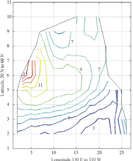
Now the opportunity presents itself to explore the seasonal variations of surface temperature a bit more than has been done in the past by extending the scope of the study to the whole North Pacific (north of 20˚N) while keeping the longitudinal variation at mid-latitudes of the eastern part of the basin in mind. At mid-latitudes across the ocean the amplitude of the seasonal variation of surface temperature at a fixed location is about 10˚C (Figure 1). That is a significant number, which is twenty times larger than the accuracy of individual ship-injec- tion temperatures, for example, and therefore needs to be understood better if possible.

What follows is based entirely on ship-injection tem-peratures averaged over five degree (latitude/longitude) squares and one month intervals and further averaged over 29 years beginning with 1947 [These 29 years of data are what I have to work with now, which appear to be sufficient for the present purposes (see Discussion)].

Figure 1. North Pacific map of the annual range of sea surface

temperature in the 29 years mean: contours in ˚C. Based on the same data set as in Figures 2 and 3.

There are literally millions of sea surface temperature measurements contained in this Namias-Scripps data set.

Maps of the North Pacific sea surface above 20˚N (Figures 2 and 3), showing regions where the highest and lowest monthly mean temperatures occur, in the long term average, have never been drawn before, to the best of my knowledge. There are no a priori expectations for what such maps may turn out to look like. Also a recent map of the mean seasonal range of surface temperature has been produced below (Figure 1) to compare with a

Figure 2. North Pacific map of the month of highest sea

sur-face temperatures in the 29 years mean: 8 = August, 9 = Sep-tember, 10 = October. Based on ship-injection temperatures for one month intervals and five degree squares over the whole North Pacific north of 20˚N.

Figure 3. North Pacific map of the month of lowest

much earlier one made in the late 1800s by Murray using data that were available to him at that time [5], which are far fewer than what are accessible here.

It would be nice to know, for their intrinsic interest alone, if maps similar to Figure 2 or 3 showing long term monthly mean air temperatures near the ground have ever been made for the North American continent, down-stream from the North Pacific, so to speak, surely adequate data to do so can easily be obtained. Is there any reason to expect broad regional differences in the month of highest or lowest mean temperatures across the US? If so, does one expect such large time lags (one to three months) between when the sun is farthest north and the warmest month of the year, or between when the sun in farthest south and the coldest month of the year, such as illustrated in Figures 2 and 3? The sun is farthest north on or about June 21 whereas the warmest month of the year varies between August and October at the sea surface throughout the North Pacific. After the sun is farthest south on December 21, one waits till February, March and even April for the coldest ocean surface tem-peratures to appear.

2. THE MAPS

In Figure 2, distinct large-scale areas are shown for August, September and October, where the highest ocean surface temperatures of the year are to be found in these monthly means in the twenty nine year average. Two equally broad bands are depicted, trending roughly from southwest to northeast: one for August and the other for September.Along a latitude line the September band lies east of the August band.A small pocket of October highs occurs in the extreme southeast. Also there is a small region of September highs in the northwest.

March is the most common month for the mean lowest sea surface temperature to take place over the North Pa-cific (Figure 3) except for a band of Februarys mostly in the middle of the ocean trending northeast/southwest. There are a few very small pockets of Februarys scat-tered around the rim of the basin and one small pocket of Aprils in the far southeastern corner.

Remarkably the seasonal range map (Figure 1) quali-tatively confirms the North Pacific part of Murray’s 1898 world chart [6] even though he dealt with extreme sea-sonal ranges instead of the mean seasea-sonal ranges used here.To cite a detail first, in the middle of the North Pa-cific on Murray’s map is a small isolated high sticking out like a sore thumb, an oddity that grabs the reader’s attention.Is it real or not?Why did he bother to put such a tiny feature in his chart?Figure 1 has a similar feature, although the contour interval between 9 and 10 would need to be made a bit smaller to bring it out distinctly. The longitudes are almost the same in both cases but the latitude is lower in Figure 1 than on Murray’s map.Also

the numerical values of the seasonal ranges are larger on Murray’s map because he was dealing with extreme sea- sonal ranges instead of the mean ranges.But the overall structure of both charts is similar.

Although it has been found that the August-February temperature difference in general gives a good approxi- mation to the seasonal range over the North Pacific [3], what was done in Figure 1 was to subtract the lowest monthly mean temperature from the highest monthly mean temperature at each five degree latitude/longitude intersection no matter which month these extremes oc- curred in.

3. DISCUSSION

If the input of solar energy to the upper layers of the ocean were the only significant factor operating, Maps 2 and 3 would not exactly look like they do. Undoubtedly the contours would be more nearly parallel to the latitude lines in the open ocean. It is likely that surface currents are also involved, but then one expects them to be quite slow in order to try to explain the large time lags of one to three months mentioned above.

Another piece of the overall puzzle that is needed for increased understanding of what is going on is provided by the surface temperature atlases [7-9]. They all show an amazing fact about the western tropics, where the highest surface temperatures anywhere in the North Pa- cific occur.But they never get any higher in summer than in winter; the highest surface temperatures are nearly independent of time.It is as if there were a governor op- erating on the surface temperature such that there is a maximum value it cannot exceed. This in spite of the self-evident notion that more solar energy, per unit area and per unit time, is absorbed by the ocean’s surface layer in summer than in winter.

relevant one.The net effect is an increase in the north/ south temperature gradient at the sea surface because the horizontal distance between heat source and heat sink is effectively reduced while the temperature difference be- tween source and sink remains about the same.As a con- sequence of the stronger north/south surface temperature gradient in summer, the northward flow of warm water, anticipated to be slow at all times, is forecast to be a bit stronger in summer than in winter.

Otherwise one has to imagine that when the sea sur- face temperature reaches a certain maximum value, if more solar energy is then added to the ocean, the excess heat is transferred directly back to the atmosphere by evaporation and conduction in a more efficient manner than was done before the maximum sea temperature was reached. This second option seems farfetched but needs to be investigated further.

There exists, in principle, another possibility for keep- ing the surface temperature constant in the western tro- pical Pacific as the absorbed solar energy increases in summer: greater downward vertical mixing of the heat in summer. Stronger summer winds would be required for this to happen.For completeness this idea, which seems very unlikely, should be addressed.

Connecting some of the above reasoning together, the most logical source of the northeastward flowing water in the wide warm current crossing mid-latitudes in every month is the large pool in the western tropics that con- tains the highest surface temperatures in the North Pa- cific at all times of the year.

To accommodate the increased absorption of solar en- ergy in the top 100 m, and to maintain the maximum sur- face temperature nearly constant in the western tropics, the wide warm current at mid-latitudes is thought to ex- pand its width westward in summer and then contract again in the fall [10].This idea is based on the evidence that the longitudinal maximum temperature, which ap- proximately marks the center of the flow, moves west in summer at mid-latitudes, most likely without significant changes to its maximum depth or average speed.

Although the wide warm current becomes even wider in summer, its maximum depth is not expected to be any greater, because the depth-scale of the current is tied to that of the maximum penetration of sunlight, both being about 100 m.Also a sluggish speed of flow is anticipated in summer and in winter for a meridional circulation driven by a heat source (in the troptics) and a cold source (near the artic) which are at the same level (sea surface) [11,12].

Returning to Figure 2, it can be noticed that in moving eastward from about the date line along a constant lati- tude, in the mid-latitude region, the mean month of war- mest temperatures progresses from August to September and even October at lower latitudes. This progression is

consistent with the eastward shift in the position of the wide warm current in the fall that slowly brings warmer water to these eastern areas and thereby extends the summer season there, roughly speaking, beyond what it otherwise would be.

Similarly, in Figure 3 when the warm current is in its farthest east position, the winter cool-down of the eastern Pacific at mid-latitudes is delayed until March while the central Pacific, to the west and outside the warm current becomes coldest sooner in February.

A small maximum in the seasonal range of surface temperature in the middle of Figure 1 has been ex-plained before by the seasonal horizontal shifting of the wide warm current [3]: the longitudinal temperature maximum in summer is located at the same place as the longitudinal minimum is in winter. In the western part of the figure is a larger maximum, similar to the one on Murray’s chart, but the origin of this feature is not known at present. It is doubtful that the Kuroshio is involved here, since it does not show up on any of the three atlases quoted above and it did not appear in a complete hydro-graphic section with closely spaced stations along 35˚N all the way from California to Japan [13].

For comparison analogous figures to Figures 1-3 have been prepared based on only twenty years of data, in- stead of twenty nine, starting also with 1947. The differ- ences between the two sets of figures are small and judged to be insignificant. Deviations will turn up, of course, with fewer and fewer years included in the mean, but this experiment was not attempted because it is not relevant to the purpose at hand.

4. ACKNOWLEDGEMENTS

Tony Sturges converted my hand drawn maps into a very nice set of

computer diagrams.Many thanks for that.The idea of making Maps 1

and 2 was sparked by a discussion with Phil Schneider. The following

reference has just come to my attention: The annual and semiannual variation of sea surface temperature in the North Pacific Ocean (Klaus Wyrtki, 1965) [14].

REFERENCES

[1] Stommel, H. (1960) The gulf stream. University of

Cali-fornia Press, Berkeley.

[2] Kenyon, K.E. (1975) Influence of longitudinal variations

in wind stress curl on the steady ocean circulation. Jour-

nal of Physical Oceanography,5, 334-346.

doi:10.1175/1520-0485(1975)005<0334:TIOLVI>2.0.CO ;2

[3] Kenyon, K.E. (1977) A large-scale longitudinal variation

in surface temperature in the North Pacific. Journal of

Physical Oceanography, 7, 256-263.

doi:10.1175/1520-0485(1977)007<0256:ALSLVI>2.0.C O;2

the North Pacific. Journal of Geophysical Research, 86,

6529-6536. doi:10.1029/JC086iC07p06529

[5] Kenyon, K.E. (1980) North Pacific sea surface

tempera-ture observations: A History, in oceanography the past. Springer-Verlag, New York, pp. 267-279.

doi:10.1007/978-1-4613-8090-0_25

[6] Murray, J. (1898) On the annual range of temperature of

the surface waters of the ocean, and its relation to other

oceanographic phenomena. The Geographical Journal,

12, 113-137. doi:10.2307/1774459

[7] US Hydrographic Office (1944), World atlas of sea sur-

face temperature. 2nd Edition, H. O. No. 225, Washing- ton, D.C.

[8] La Violette, P.E. and Seim, S.E. (1969) Monthly charts of

mean, minimum, and maximum sea surface temperature

of the North Pacific Ocean.Naval Oceanographic Office,

Washington, D.C.

[9] Robinson, M.K. and Bauer, R.A. (1971) Atlas of monthly

mean sea surface and subsurface temperature and depth

of the top of the thermoclineNorth Pacific Ocean. Fleet

Numerical Weather Central, Monterey.

[10] Kenyon, K.E. (2012) The wide warm current of the North

Pacific. Lambert Academic Publishing, Saarbrucken.

[11] Neumann, G. and Pierson, W.J. (1966) Principles of phy-

sical oceanography.Prentice-Hall, Englewood Cliffs, 230-

233.

[12] Sandstrom, J.W. (1908) Dynamische versuche mit

meer-wasser. Ann. d. Hydr. u. Marit. Meterol., 36, 6.

[13] Kenyon, K.E. (1983) Sections along 35˚N in the Pacific.

Deep-Sea Research,30, 349-369. doi:10.1016/0198-0149(83)90071-7

[14] Wyrtki, K. (1965) The annual and semiannual variation of

sea surface temperature in the North Pacific Ocean.