Munich Personal RePEc Archive
Consumption dynamics in general
equilibrium
Hall, Jamie
University of New South Wales
November 2012
Online at
https://mpra.ub.uni-muenchen.de/43933/
Nonlinear consumption dynamics in general
equilibrium
Jamie Hall
∗School of Economics University of New South Wales
November 29, 2012
Abstract
This paper explores the role of consumption habits using an estimated nonlinear dynamic stochastic general equilibrium (DSGE) model with het-eroscedastic shocks. It finds that habits interact with time-varying volatil-ity to produce a better and more plausible fit to the data. They accentuate the nonlinear character of the simple New Keynesian model to produce asymmetries between positive and negative shocks. In general equilib-rium, these effects are transmitted as much through inflation as through consumption itself.
Keywords: New Keynesian, habits, particle filter, heteroscedastic. JEL codes: E21, E32
1
Introduction
The day after the Lehmann Bros bankruptcy, a high-end Manhattan department store had its highest day of returns ever. Panicked buyers and their spouses returned luxury items as fast as they could (Shnayerson 2009). But not all types of consumption were so quick to adjust. The decline in airline ticket purchases, for instance, was much slower. In 2007, as the US economy slid into recession, and as airline ticket prices increased, so too did the number of people flying. The number of overseas trips would only decline significantly in early 2009, months after the Lehmann collapse and more than a year after the start of the economic downturn (Figure 1).
[Figure 1 about here.]
Consumption plans can be hard to change. This is not to imply that con-sumers are irrational or stupid; merely that aggregate consumption seems to
respond sluggishly to shocks. Over the last decade, medium-scale DSGE mod-els have reflected this fact by incorporating consumption habits. In other words, the consumption Euler equation at the heart of each model included dependence on a latent habit variable, which was assumed to be in log-linear proportion to the previous quarter’s consumption.
This paper develops a model which is generalised in two ways. First, the habit stock is allowed to respond to consumption in a nonlinear fashion—it can move faster or slower depending on the state of the business cycle. Second, the exogenous shocks hitting the economy have time-varying volatility. The changing size of these shocks can then interact with the nonlinear habit func-tion, which could then generate cyclical changes in the speed of demand-side responses.
Section 2 provides more background detail on the existing literature. In section 3, I describe the simple New Keynesian model used in the paper, and section 4 explains how the model can be solved and estimated in nonlinear form. The results of this estimation are described in section 5.
2
Background
Examples of medium-scale DSGE models with a significant role for consump-tion habits include Smets and Wouters (2003), Smets and Wouters (2007), Edge, Kiley, and Laforte (2008), and Andreasen (2011). They include habits in the utility function because it makes consumption slower to respond to shocks, pro-ducing hump-shaped impulse responses rather than the decay curves that are generated by a simpler model (e.g. Walsh 2003). A hump-shaped or otherwise sluggish response is consistent with evidence from vector autoregressions on US data (Christiano, Eichenbaum, and Evans 2005), and with IV regressions on data from 13 advanced countries (Carroll, Slacalek, and Sommer 2008).
In all the DSGE models just cited, the authors used a linear functional form for the habit stock, meaning that the reference level of consumption moves in loglinear proportion to last period’s consumption. In most cases, this choice was compulsory, because the models were estimated in the form of a loglinear approximation. Nonlinear solution methods are conceptually difficult and com-putationally demanding. For that reason, nonlinear estimation remains rare; examples include Fern´andez-Villaverde and Rubio-Ram´ırez (2007b), Amisano and Tristani (2010), Andreasen (2011) and Doh (2011). This paper uses a new method, described in Hall (2012), to estimate a model with a nonlinear habit response.
Consumption cannot be the only variable determining the stochastic discount factor; otherwise, with power utility, the intertemporal elasticity of consump-tion would need to be implausibly high (Mehra and Prescott 1985). This could be mitigated by using an Epstein-Zinn utility function, in which risk appetite is distinct from the intertemporal elasticity (Binsbergen, Fern´andez-Villaverde, Koijen, and Rubio-Ram´ırez 2010, Rudebusch and Swanson 2012). This paper will follow an alternative route, using a nonlinear habit response, because it cap-tures something about business cycles that seems intuitively satisfying: the idea that recessions have adisproportionately large impact on saving and spending, compared with small fluctuations during normal economic expansion. It would be interesting to see how this effect plays out in a general-equilibrium business cycle model.
Seeing a utility function with consumption habits, we may be reminded of the psychological literature on hedonic adaptation (Frederick and Loewenstein 1999, Taylor and Houthakker 2009). Certainly, much of the literature on consumption habits from the 1950s and 1960s was informed by this psychological phenomenon (see Pollak 1978, Muellbauer 1988). But one does not have to take it entirely literally as a description of consumption decision-making. Instead, consumption habits could be seen as the reduced form of a more complex model in which agents must expend time and energy to process new information. We could imagine that households receive noisy and incomplete signals of the aggregate economy (Lucas 1972, Woodford 2001). The processing of information itself could also constrain households’ planning (Mankiw and Reis 2002, Sims 2003). With that background, consumption habits can be seen as a simple and tractable representation of legitimately sluggish reactions to demand side shocks.
This paper also fits within a smaller literature on heteroscedasticity in DSGE models. Changes in volatility are important for understanding the dynamics of the economy and the appropriate policy responses (Fern´andez-Villaverde and Rubio-Ram´ırez 2010). Several papers have established that models with time-varying volatility can fit the data better than homoscedastic models (Fern´ andez-Villaverde and Rubio-Ram´ırez 2007a, Justiniano and Primiceri 2008, Amisano and Tristani 2011). From a methodological point of view, those papers are complementary to this one: they use variations on a Taylor approximation to the model solution, evaluated at the nonstochastic steady state, while this paper uses an approximation that is conditioned on the value of the state variables at each period.
3
Model
There are many possible variations on the basic New Keynesian model. I use a simplified version of the model based on Amisano and Tristani (2010) and Fern´andez-Villaverde, Gordon, Guerr´on-Quintana, and Rubio-Ram´ırez (2012).1
It includes a representative household with a utility function separable in con-sumptionctand hours workedlt; a continuum of profit-maximising goods
pro-1
ducers in monopolistic competition, with sticky prices; and a government sector that sets the nominal interest rate through a Taylor rule. Investment is not modelled, with the capital stock instead being taken as fixed.
3.1
Household utility
The model is based on the decisions of a representative household. The house-hold’s objective is to maximise utility, given by
Ut=
∞
X
h=0
βhebt+h−1
v(Ct+h, Ht+h)1−γ
1−γ − 1 1 +φL
1+φ t+h
(1)
where Ct is consumption, Ht is the external habit stock, Lt is hours worked,
andbtis an exogenous disturbance representing demand-side shocks.
My main interest is in the specification of v(C, H) and the law of motion for the habit levelHt. The first question is whether the habit stock is internal,
meaning that each household’s habit stock tomorrow is affected by its own decisions today, or external, meaning that the habit stock is not influenced by a particular household’s actions. Using a first-order approximation, the distinction between internal and external habits makes little difference to the model’s output (Dennis 2009). But in a nonlinear setting, internal habits would require a more complex treatment of heterogeneity than my solution method can currently handle. For that reason, I assume that the habit stock is purely external.
I assume that current utility depends on the amount that current consump-tion exceeds the reference level:
v(Ct, Ht) =Ct−Ht≡CtSt (2)
where St= CtCt−Ht is the surplus consumption ratio. Following Campbell and
Cochrane (1999)2, I specify the law of motion for S
tas follows:
logSt=ψt−1bct−1 (3) ψt=−k1
p
max (1−k2bct,0) (4)
Here bct is the log-deviation of Ct from its detrended steady-state level. The
function ψ measures the sensitivity of the habit stock to the detrended level of consumption;k1 andk2 are parameters that control its average size and its
sensitivity to the business cycle. The specification in equations (2) to (4), with k1>0 andk2= 0, is equivalent to a standard external habits model (Abel 1990).
Withk2 >0, it also implies that consumption habits move rapidly during bad
times, more slowly during normal times, and not at all in times of surplus.
2
In the original specification of Campbell and Cochrane (1999),bst moves in response to the detrendedchangein the log ofCt, and with an autoregresive coefficient onbst−1. I chose
As k2 → 0, the response function reverts to a standard linear proportion, as
in a standard DSGE model; and as k1 → 0, the effect of consumption habits
disappears, and the model becomes equivalent to the simplest New Keynesian model.
The maximisation of (1) is subject to a budget constraint
PtCt+Bt=WtLt+Rt−1Bt−1+Dt (5) The household’s income is derived from a nominal wageWt, a gross returnRt−1 paid on risk-free nominal bondsBt−1, and profitsDt.
3 This income can be spent
on consumption and on saving for next period. Ptis the level of the consumer
price index in periodt.
The resulting first-order conditions of the household are
λt=Etβebtλt+1
Rt
Πt+1
(6)
C−γ
t S
ψt−1(γ−1)
t =λt (7)
Wt
Pt
λt=Lφt (8)
Equation (6) is an intertemporal consumption Euler equation, connecting the marginal utility of consumptionλtwith its expected value next period, deflated
by a time preference factorβ∈(0,1) and the expected real interest rate. Πt+1
is the ratio of the consumer price index in periodt+ 1 and periodt.
Equation (7) pins down the instantaneous marginal utility of wealth. (Again, I assume that the habit stock is purely external, so that ∂St
∂Ct(i) = 0 for any
householdi.)
Equation (8) is an intratemporal optimality condition, equating the marginal disutility of labour (Lφt) to the marginal benefit of increased consumption (Wt
Ptλt).
Wages in the model are fully flexible, and there are no labour market rigidities, so this equation determines the real wage.
3.2
Inflation, interest rates, and market clearing
The supply-side and policy components of the model are standard. I assume that there is a continuum of firms in a monopolistically competitive market, each facing a constant elasticity of demandθ >1. The production function of the representative firm is
Yt(i) =AtLt(i) (9)
HereAtis a technology shock andLt(i) is the amount of labour hired by firmi.
It follows that real marginal cost for the representative firm is given by
M Ct=
Wt/Pt
At
(10)
3
I make the standard assumption that firms are able to change their price with fixed probabilityθp each period (Calvo 1983). The firm’s problem is to choose
a price in order to maximise expected profits subject to this constraint, and subject to its constant-elasticity demand curve. Following Smets and Wouters (2003), I assume that a fractionω of firms use a rule of thumb for pricing: if they are unable to recalculate their optimal price in a given quarter, they change their price to match the last quarter’s rate of inflation. This assumption helps the model to capture sluggish responses to shocks on the supply side, keeping them separate from the effects of habits on the demand side.
Let the auxiliary variablesG1,tandG2,tequal the present values of marginal
cost and marginal revenue. The profit maximisation conditions are then given by4
θG1,t= (θ−1)G2,t (11)
G1,t=M Ct+βebtθpEt
Πt+1
Πω t
θ
G1,t+1 (12)
G2,t= Π⋆t+βebtθpEt
Πt+1
Πω t
θ−1 Π⋆
t
Π⋆ t+1
G2,t+1 (13)
Here G1 is the expected present value of marginal costs, G2 is the expected
present value of marginal revenues, and Π⋆
t is the price chosen by firms with the
opportunity to reset in periodt. Aggregate CPI inflation is given by
1 =θp
Πt
Πω t−1
θ−1
+ (1−θp)(Π⋆t)1
−θ
(14)
If the model is loglinearised around its nonstochastic steady state, with steady-state inflation log Π = 0, then equations (11) to (14) collapse into the familiar New Keynesian Phillips curve.
The market clearing conditions are
Yt=Ct (15)
Bt= 0 (16)
Interest rate policy is set according to
Rt=R1
−ρr Rρrt−1
"Π
t
Π
φπ
Ct
C
φc#1−ρr
exp (mt) (17)
This is close to a standard Taylor Rule for monetary policy. The interest rate is assumed to respond to consumption, rather than GDP, since consumption is an observed endogenous variable in the model and GDP is not. The exogenous processmtis an exogenous monetary-policy shock.
4
3.3
Exogenous shocks
The model is closed by specifying the laws of motion for the exogenous processes. These are assumed to be as follows:
logAt≡at=ρaat−1+σa,tǫa,t (18) bt=ρbbt−1+σb,tǫb,t (19) mt=ρmmt−1+σm,tǫm,t (20) The volatility of the US macroeconomy appears to have changed over time. For that reason, I allow for heteroscedasticity by assuming that each volatility σi,t is determined by an independent GARCH process:
σi,t2 =α2i +βiǫ2i,t−1+γiσ
2
i,t−1 (21) This adds two free parameters,βiandγi, for each of the three exogenous shocks.
In estimating the model, I will also consider variations in which the GARCH processes are turned off (βi =γi= 0), to check whether this extra flexibility is
justified by a substantial increase in model fit.
4
Solution and estimation
I solved the model recursively using a locally linear approximation, and esti-mated it using a particle filter. For details on the mechanics of this estimation method, see Hall (2012). In brief, the idea is to take a first-order approximation of the model’s reduced-form decision rule, conditional on the previous period’s values of the exogenous forcing variables and endogenous predetermined vari-ables. Intuitively, the sequential Monte Carlo framework of particle filtering relies on representing the model’s likelihood function with the product of a series of conditional likelihoods:
p(y1:T|θ) = T
Y
t=1
p(yt|θ, y1:(t−1))
Therefore, the approximate solution of the model at time t does not need to be unconditionally accurate for all time. It only needs to maintain its validity into time (t+ 1), at which point it can be recalculated. Thus the locally linear approach can attain higher accuracy close to the current state, at the cost of a larger discrepancy in other areas of the state space—but those areas are unlikely to be reached in a single step.
quadratically to a stable answer (Fang and Saad 2009, Walker and Ni 2011). To initialise the approximation, I used the nonstochastic loglinear approximation provided by Dynare (Adjemian, Bastani, Karam´e, Juillard, Maih, Mihoubi, Perendia, Ratto, and Villemot 2012).
Since the approximate solution of the model at timetis linear (conditional on the values of the predetermined variables), it fits naturally into the frame-work of fully adapted particle filtering (Pitt and Shephard 1999). In estimating the likelihood of the model for a given value of the parameter vectorθ, we main-tain a swarm of particles to approximate the distribution of the model’s latent variables, conditional on observations up to time t. To forecast and update the model’s state vector at time t+ 1, we can use the one-step Kalman filter, conditional on each particle. In models with a high signal to noise ratio, or for models in danger of misspecification, this method is much more efficient than the standard particle filter.
In calculating the solution of the model, I ignored the zero lower bound on the nominal interest rate. This is clearly less than ideal, given that the US has reached that bound in recent quarters. The locally linear approximation becomes numerically unstable when the zero lower bound constraint is imposed. This may be related to the unusual properties of the zero lower bound: its effects are exceptionally sensitive to parameter values (Dong 2012), and it can be consistent with multiple equilibria (Braun, K¨orber, and Waki 2012). I hope that future research will be able to resolve this problem.
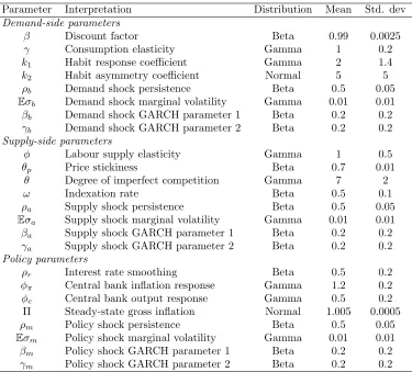
I placed fairly loose priors on most of the model’s parameters, as reported in Table 6. With the exception of the GARCH parameters, which are jointly constrained to the stable region, the priors for each parameter are independent. The priors are broadly in line with those used in previous studies (e.g. Smets and Wouters 2007). I placed loose priors on the habit response coefficients k1
andk2.5
[Table 1 about here.]
I took draws from the posterior distribution of the parameters using particle Markov chain Monte Carlo (Andrieu, Doucet, and Holenstein 2010). To assist computation, I assumed that the model’s observable variables were affected by a negligible amount of observation noise, with a standard deviation of 0.01%. For comparison with the baseline model, I estimated variants of the model without heteroscedastic shocks (βi =γi = 0) and without habits (k1 =k2= 0). I also
estimated a linear approximation of the model using standard methods. In all cases, I used the adaptive random walk Metropolis Hastings algorithm (Haario, Saksman, and Tamminen 2001). The Markov chains were initialised near the estimated posterior mode, and the proposal covariance matrix was initialised with small positive values on the diagonal. Adaptation of the proposal began after 250 draws. The posterior mode was estimated using a numerical minimiser, in the linear case, and a trial MCMC run for the nonlinear cases. I used 100
5
Here, I follow Abel (1990) in allowingk1to be greater than 1. Dennis (2009) restricted
particles in the fully adapted particle filter, because this produced estimates of the loglikelihood with a standard deviation of around 1, which is optimal for a Metropolis Hastings run (Pitt, Silva, Giordani, and Kohn 2012). I took 500,000 draws from the posterior distribution, discarding the first 400,000 as burn-in.
The observable variables of the model are logct, log Πtandrt. I used
quar-terly data from 1960Q1 to 2012Q3, a total of 211 quarters. I obtained the data from the FRED (Federal Reserve Economic Data) database from the Federal Reserve Bank of St. Louis. For consumption, I used real personal consumption expenditures (FRED code PCECC96). Following Smets and Wouters (2003) and Amisano and Tristani (2010), I substracted a loglinear trend from the con-sumption series prior to estimation. For inflation, I used the PCE deflator excluding food and energy (FRED code JCXFE PCH). I chose this measure, rather than the headline PCE deflator, because the rapid movements in food and energy prices can produce fluctuations that are difficult to capture in a sim-ple DSGE model. Both the consumption and inflation measures were seasonally adjusted prior to estimation. For the nominal interest rate I used the effective Federal Funds rate (FEDFUNDS), converted to a quarterly basis.
5
Analysis
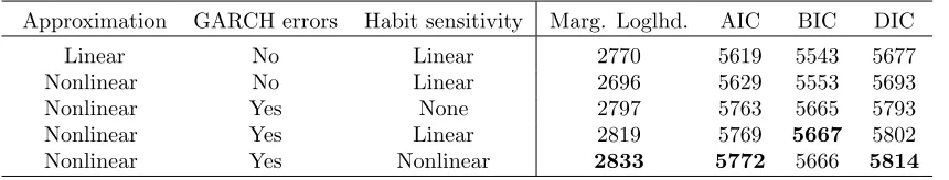
A nonlinear model with both consumption habits and time-varying volatility fits the data considerably better than models with only one of those features. This is summarised in Table 2, where I report the marginal loglikelihood of different variations of the model.6 The largest improvement in model fit comes from
allowing time-varying volatility, with habits adding further accuracy. The Ta-ble also contains three measures that penalise the model for additional free parameters, with the goal of reducing overfitting. Those measures are the Akaike Information Criterion (Akaike 1974), the Bayesian Information Criterion (Schwarz 1978) and the Deviance Information Criterion (Spiegelhalter, Best, Carlin, and Van Der Linde 2002). The AIC and DIC favour the fully nonlinear model, while the BIC narrowly prefers the nonlinear model with a linear habit response function (k2= 0 in equation 4).
[Table 2 about here.]
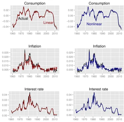
Figure 2 shows the one-step-ahead forecasts for the three observable vari-ables made by the fully nonlinear model and by the linear approximation. Un-surprisingly perhaps, the nonlinear model has a better in-sample fit than the linear version during periods of heightened volatility, such as the 1970s. The models’ in-sample fits are very similar during the Great Moderation period of 1985-2007. Both models have difficulty tracking the level of inflation for a few quarters around 1970, 1977 and 2010. A time-varying or regime-switching ver-sion of the Taylor rule may help in this regard.
6
[Figure 2 about here.]
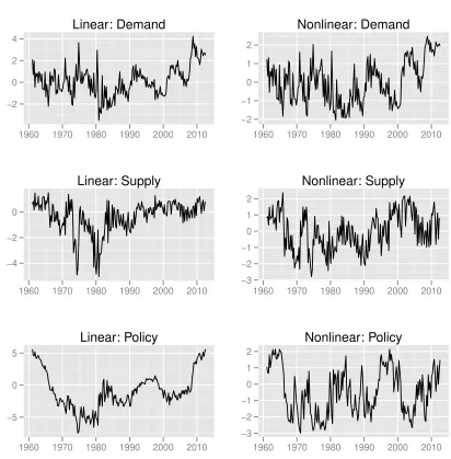
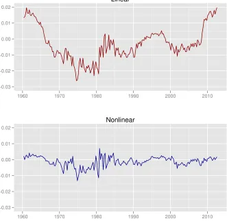
In addition to the summary measures in Table 2, one can look at the filtered residuals to see the improvement from allowing time-varying volatility. Fig-ure 3 shows the standardised residuals—that is, the estimated values of σi,tǫi,t— evaluated at the posterior mean of the parameters, for the fully nonlinear model and the linear approximation. The standardised residuals for the linear model, in the left-hand column, are clearly non-normal, showing many draws close to the origin and quite a few draws larger than 3 standard deviations. The nonlinear shocks are more reasonable in size. They show a high degree of auto-correlation, indicating that the model specification could be improved further, but their marginal distribution is not unreasonable.
[Figure 3 about here.]
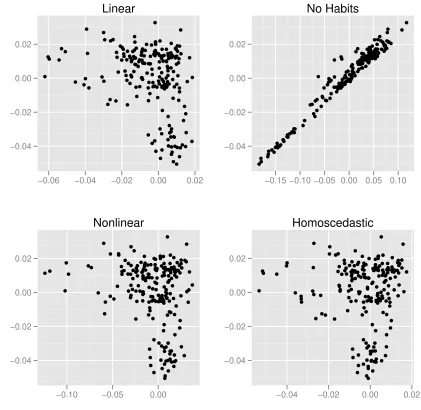
The model with GARCH errors but without habits has a reasonable marginal likelihood—higher than the linear model’s—but this overstates its ability to fit the data. Figure 4 shows the observed values of consumption in scatter plots against the model’s exogenous supply shifter at. The plots show four model
variations: the baseline model, a linear approximation, a homoscedastic model with habits, and the model with GARCH but without habits. For the last model, the observed variable shows a clear correlation with the level ofat. The
model’s estimated ‘structural supply shocks’ are little more than movements in consumption itself. Nobody would claim that this simple DSGE model is close to the truth, but the difference in the panels of Figure 4 suggests that the addition of habits improves the model specification.
[Figure 4 about here.]
The posterior distributions of the model’s structural parameters are fairly similar in the linear and nonlinear cases, but there are some important differ-ences. As shown in Table 6, the inverse Frisch labour supply elasticity φ is estimated to be higher by the nonlinear model. While the effect is small, the direction of change is interesting, since one might have expected that the model would prefer to reduce the curvature in the Phillips curve and thereby make it easier to fit the data. (With labour hours unobserved, the only noticeable effect of an increase inφ within the model is to make marginal costs respond more sharply to household marginal utility.) Additionally, the nonlinear model has a smaller estimated persistence of monetary policy shocks (ρm) and a smaller
degree of policy inertia (ρr). This may be evidence that the nonlinear model
fits the decidedly non-Gaussian interest rate series better than the linear ap-proximation can, despite the model’s lack of a zero lower bound.
[Table 3 about here.]
from the fully nonlinear model hadk2 > 0 about 85% of the time. And the
model with this kind of asymmetric response has a somewhat higher marginal likelihood than the model without it—high enough to justify the addition of an extra free parameter, at least according to the AIC and the DIC. But the esti-mated level ofk2implies a fairly small variation across the span of observations.
At the highest end of the posterior confidence interval, the habit sensitivityψ ranges between 7.1 (in 1973 Q2) and 8.1 (in 2012 Q3). This might reflect the small number of cyclical troughs in the dataset, coupled with the slow response of consumption to a shock.
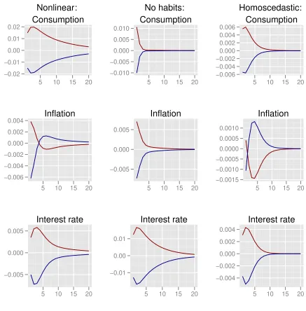
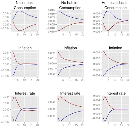
Additionally, the evidence for a nonlinear habit response function might be weak because the model already captures important asymmetries: between small and large shocks, and between positive and negative shocks. Figure 5 plots impulse responses for demand shocks of ±2 standard deviations. They are plotted at the estimated mean parameter values for the baseline model, the model without habits, and the model without time-varying volatility. (The responses are measured as deviations from a situation initialised at the non-stochastic steady state, since the adjustment to different volatility levels causes some movement in the endogenous variables.) Figure 6 repeats the exercise for supply shocks. For the first two models, I set the volatility of the shocks equal to the their estimated marginal levels. The baseline model’s inflation re-sponse to a large negative demand shock is bigger, in absolute value, than the inflation response to a large positive shock. This asymmetry is much weaker in the model without habits. Similarly, the inflation response to a large positive supply shock is a little bigger in absolute value than a large negative shock; again, the model without habits does not exhibit this asymmetry to the same extent. The explanation is that the effects of consumption habits interact with the stickiness of prices. In the presence of habits, consumption will be affected by a shock for a longer period. Therefore, with a contractionary demand shock, firms’ marginal costs will be low for longer, since households will be willing to work at a lower rate (equation 9). With a reciprocal labour-supply elasticity φ >1, there is a cyclical asymmetry in the labour-supply schedule, which is ac-centuated by price stickiness in the presence of habits. This effect is largest in the model with homoscedastic shocks; with GARCH innovations, a large shock announces a period of unusually high volatility, which causes firms to display more risk-averse behaviour.
[Figure 5 about here.]
[Figure 6 about here.]
[Figure 7 about here.]
[Figure 8 about here.]
monetary shock, particularly in inflation. Indeed, at the posterior mean of the parameters, the model without habits generates such a strong inflationary response from a large tightening in the policy stance that the nominal interest rate initially falls, to produce a real interest rate consistent with the model’s Taylor rule. The smaller size of the shocks in the model with habits could be interpreted as evidence that the model with habits fits the data better, in the sense that there is a smaller residual to be explained after the effects of aggregate supply and demand are accounted for.
6
Conclusion: What do habits do?
Consumption habits make the demand side of a DSGE model more sluggish in response to shocks, but in a nonlinear model their contribution is more impor-tant. Habits interact with time-varying volatility to produce a better and more plausible fit to the data. They accentuate the nonlinear character of the simple New Keynesian model to produce asymmetries between positive and negative shocks. In general equilibrium, these effects are transmitted as much through inflation as through consumption itself. For those reasons, a habit-response function that responds in a nonlinear way to the level of consumption appears to be redundant in a general equilibrium model.
As I mentioned in section 2, consumption habits can be seen as a rough-and-ready approximation to a more realistic model of the demand side, in which households’ slow responses to shocks are due to factors such as information processing and idiosyncratic shocks. A possible next step would be to estimate a more complex model with an explicit treatment of these factors. But the results of this model also suggest that it would be worth including a richer version of the supply side. In particular, it may be worth exploring the connection between consumption habits and inflation in a model with wage-setting rigidities and heterogeneous labour supply elasticities.
References
Abel, A. B. (1990): “Asset Prices under Habit Formation and Catching up with the Joneses,”The American Economic Review, 80(2), 38–42.
Adjemian, S., H. Bastani, F. Karam´e, M. Juillard, J. Maih, F. Mi-houbi, G. Perendia, M. Ratto, and S. Villemot (2012): “Dynare: Reference Manual, Version 4,” Dynare Working Paper 1, CEPREMAP.
Akaike, H.(1974): “A new look at the statistical model identification,”IEEE Transactions on Automatic Control, 19(6), 716 – 723.
(2011): “Exact likelihood computation for nonlinear DSGE models with heteroskedastic innovations,” Journal of Economic Dynamics and Con-trol, 35(12), 2167–2185.
Andreasen, M. M.(2011): “An Estimated DSGE Model: Explaining Varia-tion in Nominal Term Premia, Real Term Premia, and InflaVaria-tion Risk Premia,”
SSRN eLibrary.
Andrieu, C., A. Doucet, and R. Holenstein (2010): “Particle Markov chain Monte Carlo methods,”Journal of the Royal Statistical Society: Series B (Statistical Methodology), 72(3), 269–342.
Binsbergen, J. v., J. Fern´andez-Villaverde, R. S. J. Koijen,andJ. F. Rubio-Ram´ırez(2010): “The Term Structure of Interest Rates in a DSGE Model with Recursive Preferences,” Working Paper 15890, National Bureau of Economic Research.
Braun, R. A., L. M. K¨orber, and Y. Waki (2012): “Some Unpleasant Properties of Log-Linearized Solutions When the Nominal Rate Is Zero,” Working Paper 2012-5a, Federal Reserve Bank of Atlanta.
Calvo, G. A.(1983): “Staggered prices in a utility-maximizing framework,”
Journal of Monetary Economics, 12(3), 383–398.
Campbell, J. Y., and J. H. Cochrane (1999): “By Force of Habit: A Consumption-Based Explanation of Aggregate Stock Market Behavior,”
Journal of Political Economy, 107(2), 205–251.
Carroll, C. D., J. Slacalek,andM. Sommer(2008): “International Evi-dence on Sticky Consumption Growth,” Working Paper 13876, National Bu-reau of Economic Research.
Christiano, L. J., M. Eichenbaum, and C. L. Evans (2005): “Nominal Rigidities and the Dynamic Effects of a Shock to Monetary Policy,” Journal of Political Economy, 113(1), 1–45.
Cochrane, J. H.(2008): “Financial Markets and the Real Economy,” in Hand-book of the Equity Risk Premium, ed. by R. Mehra, pp. 237–325. Elsevier, San Diego.
(2011): “Presidential Address: Discount Rates,” The Journal of Fi-nance, 66(4), 1047–1108.
Dennis, R.(2009): “Consumption Habits in a New Keynesian Business Cycle Model,” Journal of Money, Credit and Banking, 41(5), 1015–1030.
Doh, T.(2011): “Yield curve in an estimated nonlinear macro model,”Journal of Economic Dynamics and Control, 35(8), 1229–1244.
Edge, R. M., M. T. Kiley, andJ.-P. Laforte(2008): “Natural rate mea-sures in an estimated DSGE model of the U.S. economy,”Journal of Economic Dynamics and Control, 32(8), 2512–2535.
Fang, H.-r., and Y. Saad (2009): “Two classes of multisecant methods for nonlinear acceleration,” Numerical Linear Algebra with Applications, 16(3), 197–221.
Fern´andez-Villaverde, J., G. Gordon, P. A. Guerr´on-Quintana,
and J. Rubio-Ram´ırez (2012): “Nonlinear Adventures at the Zero Lower Bound,” National Bureau of Economic Research Working Paper Series, No. 18058.
Fern´andez-Villaverde, J., and J. Rubio-Ram´ırez (2006): “A Baseline DSGE Model,” Mimeo, University of Pennsylvania.
(2010): “Macroeconomics and Volatility: Data, Models, and Esti-mation,” National Bureau of Economic Research Working Paper Series, No. 16618.
Fern´andez-Villaverde, J.,and J. F. Rubio-Ram´ırez(2007a): “Estimat-ing Macroeconomic Models: A Likelihood Approach,” The Review of Eco-nomic Studies, 74(4), 1059–1087.
(2007b): “How Structural Are Structural Parameters?,”National Bu-reau of Economic Research Working Paper Series, No. 13166.
Frederick, S.,andG. Loewenstein(1999): “Hedonic adaptation,” in Well-being: The foundations of hedonic psychology, ed. by D. Kahneman, E. Di-ener,andN. Schwarz, pp. 302–329. Russell Sage Foundation, New York, NY, US.
Gal´ı, J.(2008): Monetary Policy, Inflation, and the Business Cycle: An In-troduction to the New Keynesian Framework. Princeton University Press.
Gelfand, A. E., and D. K. Dey (1994): “Bayesian Model Choice: Asymp-totics and Exact Calculations,”Journal of the Royal Statistical Society. Series B (Methodological), 56(3), 501–514.
Geweke, J. (1999): “Using simulation methods for Bayesian econometric models: inference, development,and communication,” Econometric Reviews, 18(1), 1–73.
Haario, H., E. Saksman,andJ. Tamminen(2001): “An Adaptive Metropo-lis Algorithm,”Bernoulli, 7(2), 223–242.
Hall, R. E. (1978): “Stochastic Implications of the Life Cycle-Permanent Income Hypothesis: Theory and Evidence,” Journal of Political Economy, 86(6), 971–987.
Justiniano, A.,and G. E. Primiceri(2008): “The Time-Varying Volatility of Macroeconomic Fluctuations,” The American Economic Review, 98(3), 604–641.
Lucas, R. E.(1972): “Expectations and the neutrality of money,”Journal of Economic Theory, 4(2), 103–124.
Mankiw, N. G.,andR. Reis(2002): “Sticky Information versus Sticky Prices: A Proposal to Replace the New Keynesian Phillips Curve,” The Quarterly Journal of Economics, 117(4), 1295–1328.
Mehra, R.,and E. C. Prescott(1985): “The equity premium: A puzzle,”
Journal of Monetary Economics, 15(2), 145–161.
Muellbauer, J. (1988): “Habits, Rationality and Myopia in the Life Cy-cle Consumption Function,” Annals of Economics and Statistics / Annales d’ ´Economie et de Statistique, (9), 47–70.
Pitt, M. K., andN. Shephard (1999): “Filtering via Simulation: Auxiliary Particle Filters,” Journal of the American Statistical Association, 94(446), 590–599.
Pitt, M. K., R. d. S. Silva, P. Giordani,andR. Kohn(2012): “On some properties of Markov chain Monte Carlo simulation methods based on the particle filter,” Journal of Econometrics, 171(2), 134–151.
Pollak, R. A.(1978): “Endogenous Tastes in Demand and Welfare Analysis,”
The American Economic Review, 68(2), 374–379.
Rudebusch, G. D., and E. T. Swanson (2012): “The Bond Premium in a DSGE Model with Long-Run Real and Nominal,”American Economic Jour-nal: Macroeconomics, 4(1), 105–143.
Schwarz, G.(1978): “Estimating the Dimension of a Model,” The Annals of Statistics, 6(2), 461–464.
Shnayerson, M.(2009): “Profiles in Panic,”Vanity Fair, (January).
Sims, C. A.(2003): “Implications of rational inattention,”Journal of Monetary Economics, 50(3), 665–690.
Smets, F., and R. Wouters (2007): “Shocks and Frictions in US Business Cycles: A Bayesian DSGE Approach,” American Economic Review, 97(3), 586–606.
Spiegelhalter, D. J., N. G. Best, B. P. Carlin,andA. Van Der Linde
(2002): “Bayesian measures of model complexity and fit,” Journal of the Royal Statistical Society: Series B (Statistical Methodology), 64(4), 583–639.
Taylor, L. D., and H. S. Houthakker (2009): Consumer Demand in the United States: Prices, Income, and Consumption Behavior. Springer.
Walker, H. F., and P. Ni (2011): “Anderson Acceleration for Fixed-Point Iterations,” SIAM J. Numer. Anal., 49(4), 1715–1735.
Walsh, C. E.(2003): Monetary Theory and Policy. MIT Press, 2nd edn.
Woodford, M. (2001): “Imperfect Common Knowledge and the Effects of Monetary Policy,” Working Paper 8673, National Bureau of Economic Re-search.
List of Figures
1 Year-on-year growth in US citizen air traffic to overseas regions, Canada, and Mexico. Shading shows NBER recession dates.
Sources: Office of Travel and Tourism Industries; NBER. . . 18 2 In-sample fit of the linear model (red) and the nonlinear model
(blue). The charts show the models’ one-step-ahead forecasts for the three observable variables, using the full sample to estimate the parameters. Actual observations are in black. . . 19 3 Standardised residuals of the linear model and the fully nonlinear
model. If the model specification were correct, then these would look like a series of iid N(0,1) draws. . . 20 4 Scatter plots of the observed values of consumption against the
estimated values of the supply-shock processbat. . . 21
5 Impulse responses from a 2-σsized increase in the demand-shock process bgt and a 2-σ decrease. These estimates were calculated
at the posterior mean for each model. Left-hand column: fully nonlinear model; centre column: model with k1 =k2= 0;
right-hand column: model withβi=γi = 0. . . 22
6 Impulse responses from a 2-σsized increase in the supply-shock process bat and a 2-σ decrease. These estimates were calculated
at the posterior mean for each model. Left-hand column: fully nonlinear model; centre column: model with k1 =k2= 0;
right-hand column: model withβi=γi = 0. . . 23
7 Impulse responses from an increase and decrease in the policy-shock process mbt sufficient to move the interest rate by about
25 basis points. These estimates were calculated at the posterior mean for each model. Left-hand column: fully nonlinear model; centre column: model with k1 = k2 = 0; right-hand column:
model with βi=γi= 0. . . 24
8 Estimated level of the policy-shock process mbtfor the linear and
−10 −5 0 5 10
2006 2007 2008 2009 2010
[image:19.612.222.392.269.467.2]%
Figure 1: Year-on-year growth in US citizen air traffic to overseas regions, Canada, and Mexico. Shading shows NBER recession dates.
−0.04 −0.02 0.00 0.02
Actual
Linear
1960 1970 1980 1990 2000 2010
Consumption
0.005 0.010 0.015 0.020 0.025
1960 1970 1980 1990 2000 2010
Inflation
0.00 0.01 0.02 0.03 0.04
1960 1970 1980 1990 2000 2010
Interest rate
−0.04 −0.02 0.00 0.02
Nonlinear
1960 1970 1980 1990 2000 2010
Consumption
0.005 0.010 0.015 0.020 0.025
1960 1970 1980 1990 2000 2010
Inflation
0.00 0.01 0.02 0.03 0.04
1960 1970 1980 1990 2000 2010
[image:20.612.139.551.160.566.2]Interest rate
−2 0 2 4
1960 1970 1980 1990 2000 2010
Linear: Demand
−4 −2 0
1960 1970 1980 1990 2000 2010
Linear: Supply
−5 0 5
1960 1970 1980 1990 2000 2010
Linear: Policy
−2 −1 0 1 2
1960 1970 1980 1990 2000 2010
Nonlinear: Demand
−3 −2 −1 0 1 2
1960 1970 1980 1990 2000 2010
Nonlinear: Supply
−3 −2 −1 0 1 2
1960 1970 1980 1990 2000 2010
[image:21.612.140.552.158.577.2]Nonlinear: Policy
−0.04 −0.02 0.00 0.02 ● ● ● ●● ● ● ●●● ● ● ●● ● ● ● ● ● ● ● ● ● ● ● ●●● ● ●● ● ● ● ● ● ● ● ● ●● ● ● ● ●● ● ● ● ● ● ● ● ● ● ● ● ● ● ● ● ● ● ● ● ● ● ● ● ● ● ● ● ● ● ● ● ● ● ● ● ● ● ● ●● ● ● ● ● ● ● ● ● ● ● ● ● ● ● ● ● ● ● ● ● ● ● ● ● ● ● ● ● ● ●●● ● ● ● ● ● ● ● ● ● ● ● ● ● ● ●●● ● ●● ● ● ●●●●● ●●●● ● ●● ● ● ● ● ● ● ● ● ● ● ● ● ●●●● ● ● ●● ●● ● ● ● ●● ● ●● ●● ● ●● ● ● ● ● ● ● ● ● ● ● ● ● ● ● ● ● ● ● ● ● ● ●●
−0.06 −0.04 −0.02 0.00 0.02
Linear
−0.04 −0.02 0.00 0.02 ● ● ● ●● ● ● ●● ● ● ●●● ● ● ● ● ● ● ● ● ● ● ●●●● ● ●● ● ● ● ● ● ● ●● ●● ● ● ● ● ● ● ● ● ● ● ● ● ● ● ● ● ● ● ● ● ● ● ● ● ●●●● ● ● ● ● ● ● ● ● ● ● ● ● ● ● ● ● ● ● ● ● ● ● ● ● ● ● ● ● ● ● ● ● ● ● ● ● ● ● ● ● ● ● ● ● ● ● ● ● ● ● ● ● ● ● ● ● ● ● ● ● ● ● ● ●●●● ●● ● ● ●●●● ●●●● ● ● ● ● ● ● ● ● ● ● ● ●● ● ● ● ● ● ● ● ● ● ●● ●●● ● ● ●● ● ●● ●● ●●● ● ● ● ● ● ● ● ● ● ● ● ● ●●●●● ● ● ● ● ● ●−0.10 −0.05 0.00
Nonlinear
−0.04 −0.02 0.00 0.02 ● ● ● ●● ● ● ●●● ● ●●●● ● ● ● ● ●● ● ●● ●●● ●● ● ● ● ● ● ●● ● ● ● ● ●● ● ● ●● ● ● ● ● ● ● ● ● ● ● ● ● ● ● ● ●● ● ● ●● ●● ●●● ● ● ● ● ● ● ● ● ●● ● ● ● ● ● ● ● ● ● ● ● ● ● ●●● ● ● ● ● ● ● ● ● ● ●● ● ● ● ●●● ●●● ● ● ● ● ● ●● ● ●●●● ● ● ● ●●●●●● ●●●●●●●●● ● ● ●● ●● ●● ●● ●● ● ● ● ● ● ● ● ● ●● ● ● ●●● ● ●●● ● ●● ● ● ●●● ● ● ● ● ● ● ● ● ● ●● ●●● ●● ● ● ● ● ● ● ●−0.15 −0.10 −0.05 0.00 0.05 0.10
No Habits
−0.04 −0.02 0.00 0.02 ● ● ● ●● ● ● ●●● ● ● ●● ● ● ● ● ● ● ● ● ● ● ● ●●●● ●● ● ● ● ● ● ● ● ● ●● ● ● ● ●● ● ● ● ● ● ● ● ● ● ● ● ● ● ● ● ●● ● ● ● ● ● ● ● ● ● ● ● ● ● ● ● ● ● ● ● ● ● ● ● ●● ● ● ● ● ● ● ● ● ● ● ● ● ● ● ● ● ● ● ● ● ● ● ● ● ● ● ● ● ● ● ● ● ● ● ● ● ● ● ● ●● ●● ● ●●●● ●● ● ● ●●●●●●●● ● ● ●● ● ● ● ● ● ● ● ● ● ●● ● ● ● ● ● ● ● ●● ●● ● ● ● ●● ● ●● ●●● ●●● ● ● ● ● ● ● ● ● ● ● ● ● ● ●●● ● ●● ● ●●−0.04 −0.02 0.00 0.02
[image:22.612.136.557.178.588.2]Homoscedastic
−0.02 −0.01 0.00 0.01 0.02
5 10 15 20
Nonlinear:
Consumption
−0.006 −0.004 −0.002 0.000 0.002 0.004
5 10 15 20
Inflation
−0.005 0.000 0.005
5 10 15 20
Interest rate
−0.010 −0.005 0.000 0.005 0.010
5 10 15 20
No habits:
Consumption
−0.005 0.000 0.005
5 10 15 20
Inflation
−0.01 0.00 0.01
5 10 15 20
Interest rate
−0.006 −0.004 −0.002 0.000 0.002 0.004 0.006
5 10 15 20
Homoscedastic:
Consumption
−0.0015 −0.0010 −0.0005 0.0000 0.0005 0.0010
5 10 15 20
Inflation
−0.004 −0.002 0.000 0.002 0.004
5 10 15 20
[image:23.612.141.578.135.579.2]Interest rate
Figure 5: Impulse responses from a 2-σ sized increase in the demand-shock processbgtand a 2-σdecrease. These estimates were calculated at the posterior
−0.004 −0.002 0.000 0.002 0.004
5 10 15 20
Nonlinear:
Consumption
−0.004 −0.002 0.000 0.002 0.004
5 10 15 20
Inflation
−0.004 −0.002 0.000 0.002 0.004
5 10 15 20
Interest rate
−0.015 −0.010 −0.005 0.000 0.005 0.010 0.015
5 10 15 20
No habits:
Consumption
−0.002 −0.001 0.000 0.001 0.002
5 10 15 20
Inflation
−0.002 0.000 0.002
5 10 15 20
Interest rate
−0.006 −0.004 −0.002 0.000 0.002 0.004
5 10 15 20
Homoscedastic:
Consumption
−0.004 −0.002 0.000 0.002 0.004
5 10 15 20
Inflation
−0.004 −0.002 0.000 0.002 0.004 0.006
5 10 15 20
[image:24.612.143.577.137.574.2]Interest rate
Figure 6: Impulse responses from a 2-σsized increase in the supply-shock process
batand a 2-σdecrease. These estimates were calculated at the posterior mean
−0.005 0.000 0.005
5 10 15 20
Nonlinear:
Consumption
−0.002 −0.001 0.000 0.001 0.002
5 10 15 20
Inflation
−0.002 −0.001 0.000 0.001 0.002
5 10 15 20
Interest rate
−0.010 −0.005 0.000 0.005 0.010
5 10 15 20
No habits:
Consumption
−0.015 −0.010 −0.005 0.000 0.005 0.010
5 10 15 20
Inflation
−0.003 −0.002 −0.001 0.000 0.001 0.002
5 10 15 20
Interest rate
−0.005 0.000 0.005 0.010
5 10 15 20
Homoscedastic:
Consumption
−0.004 −0.002 0.000 0.002 0.004
5 10 15 20
Inflation
−0.002 −0.001 0.000 0.001 0.002
5 10 15 20
[image:25.612.132.578.136.564.2]Interest rate
Figure 7: Impulse responses from an increase and decrease in the policy-shock processmbtsufficient to move the interest rate by about 25 basis points. These
estimates were calculated at the posterior mean for each model. Left-hand column: fully nonlinear model; centre column: model withk1=k2 = 0;
−0.03 −0.02 −0.01 0.00 0.01 0.02
1960 1970 1980 1990 2000 2010
Linear
−0.03 −0.02 −0.01 0.00 0.01 0.02
1960 1970 1980 1990 2000 2010
[image:26.612.146.477.223.549.2]Nonlinear
Figure 8: Estimated level of the policy-shock processmbtfor the linear and fully
List of Tables
1 Prior distributions . . . 27 2 Measures of in-sample fit. Boldface indicates best model
Parameter Interpretation Distribution Mean Std. dev
Demand-side parameters
β Discount factor Beta 0.99 0.0025 γ Consumption elasticity Gamma 1 0.2 k1 Habit response coefficient Gamma 2 1.4
k2 Habit asymmetry coefficient Normal 5 5
ρb Demand shock persistence Beta 0.5 0.05 Eσb Demand shock marginal volatility Gamma 0.01 0.01
βb Demand shock GARCH parameter 1 Beta 0.2 0.2
γb Demand shock GARCH parameter 2 Beta 0.2 0.2
Supply-side parameters
φ Labour supply elasticity Gamma 1 0.5 θp Price stickiness Beta 0.7 0.01
θ Degree of imperfect competition Gamma 7 2 ω Indexation rate Beta 0.5 0.1 ρa Supply shock persistence Beta 0.5 0.05 Eσa Supply shock marginal volatility Gamma 0.01 0.01
βa Supply shock GARCH parameter 1 Beta 0.2 0.2
γa Supply shock GARCH parameter 2 Beta 0.2 0.2
Policy parameters
ρr Interest rate smoothing Beta 0.5 0.2
φπ Central bank inflation response Gamma 1.2 0.2
φc Central bank output response Gamma 0.5 0.2
Π Steady-state gross inflation Normal 1.005 0.0005 ρm Policy shock persistence Beta 0.5 0.05 Eσm Policy shock marginal volatility Gamma 0.01 0.01
βm Policy shock GARCH parameter 1 Beta 0.2 0.2
γm Policy shock GARCH parameter 2 Beta 0.2 0.2
[image:28.612.138.513.122.461.2]Note: In the nonlinear approximation, each pair of GARCH parameters βi and γi was restricted to the stable region, 0≤βi+γi<1.
Approximation GARCH errors Habit sensitivity Marg. Loglhd. AIC BIC DIC Linear No Linear 2770 5619 5543 5677 Nonlinear No Linear 2696 5629 5553 5693 Nonlinear Yes None 2797 5763 5665 5793 Nonlinear Yes Linear 2819 5769 5667 5802
[image:29.612.133.563.339.421.2]Nonlinear Yes Nonlinear 2833 5772 5666 5814
Parameter Linear Nonlinear Mean 90% CI Mean 90% CI
Demand-side parameters
β 0.993 [0.992,0.995] 0.994 [0.993,0.995] γ 1.51 [1.3,1.7] 1.4 [1.3,1.5] k1 5.32 [3.5,7.9] 7.51 [5.5,9.2]
k2 — — 0.667 [-0.75,1.9]
ρb 0.564 [0.49,0.63] 0.475 [0.42,0.54] Eσb 0.00802 [0.0069,0.0094] 0.0199 [0.015,0.026]
βb — — 0.215 [0.13,0.3]
γb — — 0.575 [0.45,0.7]
Supply-side parameters
φ 1.44 [0.98,1.9] 1.92 [1.4,2.3] θp 0.708 [0.69,0.72] 0.734 [0.72,0.75]
θ 9.25 [5.2,14] 9.65 [6,13] ω 0.394 [0.26,0.55] 0.424 [0.32,0.54] ρa 0.551 [0.46,0.64] 0.536 [0.46,0.59] Eσa 0.0123 [0.0094,0.016] 0.0199 [0.013,0.032]
βa — — 0.149 [0.1,0.22]
γa — — 0.842 [0.76,0.89]
Policy parameters
ρr 0.742 [0.59,0.89] 0.697 [0.64,0.74]
φπ 1.24 [1,1.5] 0.627 [0.53,0.72]
φc 0.39 [0.26,0.53] 0.0732 [0.047,0.11]
Π 1.0059 [1.005,1.007] 1.0054 [1.005,1.006] ρm 0.864 [0.82,0.9] 0.653 [0.59,0.71] Eσm 0.00351 [0.003,0.0041] 0.00518 [0.0039,0.0066]
βm — — 0.24 [0.18,0.3]
[image:30.612.156.452.125.473.2]γm — — 0.671 [0.6,0.76]