Munich Personal RePEc Archive
Identification-robust inference for
endogeneity parameters in linear
structural models
Doko Tchatoka, Firmin and Dufour, Jean-Marie
McGill University, University of Tasmania, Department of
Economics, Hobart, Australia
16 August 2012
Online at
https://mpra.ub.uni-muenchen.de/40695/
Identification-robust inference for endogeneity parameters in
linear structural models
∗Firmin Doko Tchatoka† University of Tasmania
Jean-Marie Dufour‡ McGill University August 2012
∗The authors thank Marine Carrasco, Jan Kiviet and Benoit Perron for several useful comments. This work was
supported by the William Dow Chair in Political Economy (McGill University), the Bank of Canada (Research Fellow-ship), a Guggenheim Fellowship, a Konrad-Adenauer Fellowship (Alexander-von-Humboldt Foundation, Germany), the Canadian Network of Centres of Excellence [program onMathematics of Information Technology and Complex Systems (MITACS)], the Natural Sciences and Engineering Research Council of Canada, the Social Sciences and Humanities Research Council of Canada, and the Fonds de recherche sur la société et la culture (Québec).
†School of Economics and Finance, University of Tasmania, Private Bag 85, Hobart TAS 7001, Tel: +613 6226
7226, Fax:+61 3 6226 7587; e-mail: [email protected]. Homepage: http://www.fdokotchatoka.com
‡William Dow Professor of Economics, McGill University, Centre interuniversitaire de recherche en analyse des
//
ABSTRACT
We provide a generalization of the Anderson-Rubin (AR) procedure for inference on parameters which represent the dependence between possibly endogenous explanatory variables and distur-bances in a linear structural equation (endogeneity parameters). We focus on second-order depen-dence and stress the distinction betweenregressionandcovariance endogeneity parameters. Such parameters have intrinsic interest (because they measure the effect of “common factors” which induce simultaneity) and play a central role in selecting an estimation method (because they deter-mine “simultaneity biases” associated with least-squares methods). We observe that endogeneity parameters may not identifiable and we give the relevant identification conditions. We develop identification-robust finite-sample tests for joint hypotheses involving structural and regression en-dogeneity parameters, as well as marginal hypotheses on regression enen-dogeneity parameters. For Gaussian errors, we provide tests and confidence sets based on standard-type Fisher critical val-ues. For a wide class of parametric non-Gaussian errors (possibly heavy-tailed), we also show that exact Monte Carlo procedures can be applied using the statistics considered. As a special case, this result also holds for usual AR-type tests on structural coefficients. For covariance endogeneity parameters, we supply an asymptotic (identification-robust) distributional theory. Tests for partial exogeneity hypotheses (for individual potentially endogenous explanatory variables) are covered as instances of the class of proposed procedures. The proposed procedures are applied to two empiri-cal examples: the relation between trade and economic growth, and the widely studied problem of returns to education.
Key words: Identification-robust confidence sets; endogeneity; AR-type statistic; projection-based techniques; partial exogeneity test.
Contents
List of Definitions, Assumptions, Propositions and Theorems iii
1. Introduction 1
2. Framework: endogeneity parameters and their identification 3
2.1. Identification of endogeneity parameters . . . 4
2.2. Statistical problems . . . 8
3. Finite-sample inference for regression endogeneity parameters 9 3.1. AR-type tests forβ with possibly non-Gaussian errors . . . 11
3.2. Inference onθ . . . 13
3.3. Joint inference onβand regression endogeneity parameters . . . 15
3.4. Confidence sets for regression endogeneity parameters . . . 15
4. Asymptotic theory for inference on endogeneity parameters 18 5. Empirical applications 20 5.1. Trade and growth . . . 20
5.2. Education and earnings . . . 21
6. Conclusion 23
List of Tables
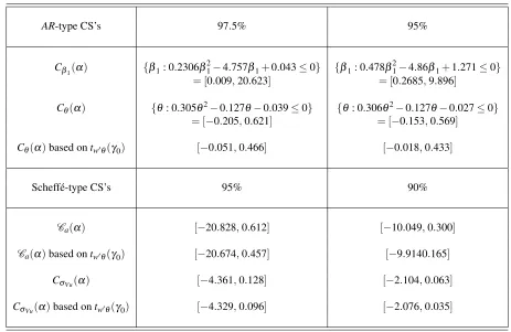
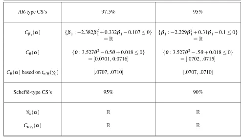
1 Projection-based confidence sets for different parameters in growth model . . . . 22 2 Projection-based confidence sets for different parameters in earning equation . . . 24
List of Figures
List of Definitions, Assumptions, Propositions and Theorems
1.
Introduction
Instrumental variable (IV) regressions are typically motivated by the fact that “explanatory vari-ables” may be correlated with the error term, so least-squares methods yield biased inconsistent estimators of model coefficients. Such IV parameter estimates can be interpreted as measures of the relationship between variables, once the “effect” of common “driving” (or “exogenous”) variables has been eliminated. Even though coefficients estimated in this way may have interesting inter-pretations from the viewpoint of economic theory, inference on such “structural parameters” raises identification difficulties. Further, it is well known that IV estimators may be very imprecise, and inference procedures (such as tests and confidence sets) can be highly unreliable, especially when instruments are weakly associated with model variables (weak instruments). This has led to a large literature aimed at producing reliable inference in the presence of weak instruments; see the reviews of Stock, Wright and Yogo (2002) and Dufour (2003).
Research on weak instruments has focused on inference for the coefficients of endogenous vari-ables in so-called “IV regressions”. This leaves out the parameters which specifically determine simultaneity features, such as the covariances between endogenous explanatory variables and dis-turbances. These parameters can be of interest for several reasons. First, they provide direct mea-sures of the importance of “common factors” which induce simultaneity. Such factors are in a sense “left out” from “structural equations”, but they remain “hidden” in “structural disturbances”. For example, in a wide set of economic models, they may represent unobserved latent variables, such as “surprise variables” which play a role in models with expectations [see Barro (1977), Dufour and Jasiak (2001)]. Second, the simultaneity covariance (or regression) coefficients determine the estimation bias of least-squares methods. Information on the size of such biases can be useful in interpreting least-squares estimates and related statistics. Third, information on the parameters of hidden variables (which induce simultaneity) may be important for selecting statistical procedures. Even if instruments are “strong”, it is well known that IV estimators may be considerably less effi-cient than least-squares estimators; see Kiviet and Niemczyk (2007) and Doko Tchatoka and Dufour (2011). Indeed, this may be the case even when endogeneity is present. If a variable is not correlated (or only weakly correlated) with the error term, instrumenting it can lead to sizable efficiency losses in estimation. Assessing when and which variables should be instrumented is an important issue for the estimation of structural models.
In this paper, we stress the view that linear structural models (IV regressions) can be interpreted as regressions with missing regressors. If the missing regressors were included, there would be no simultaneity bias, so no correction for simultaneity – such as IV methods – would be needed. This feature allows one to define a model transformation that maps a linear structural equation (with simultaneity) to a linear regression where all the explanatory variables are uncorrelated with the error term. We call this transformed equation theorthogonalized structural equation. Interestingly, the latter is not a reduced-form equation. Rather, the orthogonalized structural equation still involves the structural parameters of interest, but also includesendogeneity parameterswhich are “hidden” in the original structural equation. We focus here on this orthogonalized structural equation.
can be applied to the orthogonalized equation. This allows one to make inference jointly on both the parameters of the original structural equation and endogeneity parameters. Two types of endo-geneity parameters are considered:regression endogeneity parametersandcovariance endogeneity parameters. Under standard conditions, where instruments are strictly exogenous and errors are Gaussian, the tests and confidence sets derived in this way are exact. The proposed methods do not require identification assumptions, so they can be described asidentification-robust. For more general inference on transformations of the parameters of the orthogonalized structural equation, we propose projection methods, for such techniques allow for a simple finite-sample distributional theory and preserve robustness to identification assumptions.
To be more specific, we consider a model of the form
y=Yβ+X1γ+u
where y is an observed dependent variable,Y is a matrix of observed (possibly) endogenous re-gressors, and X1 is a matrix of exogenous variables. We observe that AR-type procedures may
be applied to test hypotheses on the transformed parameter θ =β+a, where a represents re-gression coefficients of u on the reduced-form errors ofY (regression endogeneity parameters). Identification-robust inference on a itself is then derived by exploiting the possibility of making identification-robust inference on β.Then, inference on covariances (say σVu) betweenu andY
(covariance endogeneity parameters) can be derived by considering appropriate linear transforma-tions ofa.
We stress that regression and covariance endogeneity parameters – though theoretically related – play distinct but complementary roles: regression endogeneity parameters represent the effect of reduced-form innovations ony, while covariance endogeneity parameters determine the need to in-strument different variables inY. WhenσVu=0,Y can be treated as exogenous (so IV estimation
is not warranted). So-called exogeneity tests typically test the hypothesisσVu=0.It is easy to see
thatσVu=0 if and only ifa=0 (provided the covariance matrix between reduced-form errors is
nonsingular), but the relationship is more complex in other cases. In this paper, we emphasize cases wherea6=0.Due to the failure of the exogeneity hypothesis, the distributions of various test statis-tics are much more complex. Interestingly, it is relatively easy to produce finite-sample inference ona, but not onσVu. So, forσVu, we only propose asymptotically valid tests and confidence sets.
By allowinga6=0 (orσVu6=0), we extend earlier results on exogeneity tests, which focus on
the null hypothesisHa:a=0. The literature on this topic, is considerable; see, for example, Durbin
(1954), Wu (1973, 1974, 1983a, 1983b), Revankar and Hartley (1973), Farebrother (1976), Haus-man (1978), Revankar (1978), Dufour (1979, 1987), Hwang (1980), Kariya and Hodoshima (1980), Hausman and Taylor (1981), Spencer and Berk (1981), Nakamura and Nakamura (1981), Engle (1982), Holly (1982), Reynolds (1982), Smith (1984), Staiger and Stock (1997), Doko Tchatoka and Dufour (2010, 2011). By contrast, we consider here the problem of testing any value ofa(or
σVu) and build confidence sets for these parameters. By allowing weak instruments, we extend the
results in Dufour (1987) where Wald-type tests and confidence sets are proposed for inference on
aandσVu,under assumptions which exclude weak instruments. Finally, by considering inference
on aandσVu, we extend a procedure proposed in Dufour and Jasiak (2001) for inference on the
On exploiting results from Dufour and Taamouti (2005, 2007), we supply analytical forms for the proposed confidence sets, and we give the necessary and sufficient conditions under which they are bounded. These results can be used to assess partial exogeneity hypotheses even when identification is deficient or weak.
In order to allow for alternative assumptions on error distributions, we show that the proposed AR-type statistics are pivotal as long as the errors follow a completely specified distribution (up to an unknown scale parameter), which may be non-Gaussian. Under such conditions, exact Monte Carlo tests can be performed without a Gaussian assumptions [as described in Dufour (2006)]. On allowing for more general error distributions and weakly exogenous instruments (along with standard high-level asymptotic assumptions), we also show that the proposed procedures remain asymptotically valid and identification-robust.
Finally, we apply the proposed methods to two empirical examples, previously considered in Dufour and Taamouti (2007): a study of the relationship between trade and economic growth [Frankel and Romer (1999)], and the widely considered example of returns to education [Bound, Jaeger and Baker (1995)].
The paper is organized as follows. Section 2 formulates the model considered. Section 3 presents the finite-sample theory for inference on regression endogeneity parameters. Section 4 discusses asymptotic theory and inference for covariance endogeneity parameters. Section 5 illus-trates the theoretical results through two empirical applications: a model of the relationship between trade and growth model, and returns to schooling. We conclude in Section 6. Proofs are presented in appendix.
Throughout the paper, Im stands for the identity matrix of order m. For any full rank T×m
matrixA, P(A) =A(A′A)−1A′ is the projection matrix on the space spanned by the columns ofA,
M(A) =IT−P(A),andvec(A) is the(T m)×1 dimensional column vectorization ofA. For any
squared matrixB,the notation B>0 means that B is positive definite (p.d.), whileB≥0 means it is positive semidefinite (p.s.d.). Finally, “→p ” stands for convergence in probability while “ →L ” is for convergence in distribution. Finally,kAkis the Euclidian norm of a vector or matrix,i.e., kAk= [tr(A′A)]12.
2.
Framework: endogeneity parameters and their identification
We consider a standard linear structural equation of the form:
y=Yβ+X1γ+u (2.1)
whereyis aT×1 vector of observations on a dependent variable,Yis aT×Gmatrix of observations on (possibly) endogenous explanatory variables(G≥1),X1is aT×k1full-column-rank matrix of
strictly exogenous variables, u= [u1, . . . ,uT]′ is a vector of structural disturbances, β and γ are
G×1 andk1×1 unknown coefficient vectors. Further,Y satisfies the model:
where X2 is a T ×k2 matrix of observations on exogenous variables (instruments), X = [X1,X2]
has full-column rank k =k1+k2, Π1and Π2 are k1×G and k2×G coefficient matrices, Π =
[Π1,Π2],andV = [V1, . . . ,VT]′ is aT×Gmatrix of reduced-form disturbances. Equation (2.1) is
the “structural equation” of interest, while (2.2) represents the “reduced form” forY.On substituting (2.2) into (2.1) and reexpressingyin terms of exogenous variables, we get the reduced form fory:
y=X1π1+X2π2+v (2.3)
whereπ1=γ+Π1β, π2=Π2β, andv=Vβ+u= [v1, . . . ,vT]′.
When the errors uandV have finite zero means (although this assumption could easily be re-placed by another “centering assumption”, such as zero medians), the usual necessary and sufficient condition for identification ofβ in (2.1)-(2.2) is:
rank(Π2) =G. (2.4)
IfΠ2=0,the instrumentsX2are irrelevant, andβ is completely unidentified. If 1≤rank(Π2)<G,
β is not identifiable, but some linear combinations of the elements ofβare identifiable [see Dufour and Hsiao (2008)]. IfΠ2is close not to have full rank [e.g., if some eigenvalues ofΠ2′Π2are close to
zero], some linear combinations ofβ are ill-determined by the data, a situation often called “weak identification” in this type of setup [see Dufour (2003)].
2.1. Identification of endogeneity parameters
We now wish to represent the fact thatuandV are not independent and may be correlated, taking into account the fact that structural parameters (such as β andγ)may not be identifiable. In this context, it is important to note that the “structural error”ut is not uniquely determined by the data
when identification conditions for β and γ do not hold. For that, it will be useful to consider two alternative setups for the disturbance distribution: (A) in the first one, the disturbance vectors
(ut,Vt′)′have common finite second moments (structural homoskedasticity); (A) in the second one,
we allow for a large amount of heterogeneity in the distributions of reduced-form errors ( reduced-form heterogeneity). The second setup is clearly more appropriate for practical work, and we wish to go as far as possible in that direction. But it will be illuminating to consider first the more restrictive assumption.
In setup A, we suppose that:
the vectorsUt= (ut,Vt′)′,t=1, . . . ,T,all have mean zero and finite covariance matrix (2.5)
ΣU=E
UtU
′ t = σ2
u σVu′
σVu ΣV
(2.6)
whereΣV =E
VtV
′
t
is nonsingular. In this case, the reduced-form errorsWt= (vt,Vt′)′,t=1, . . . ,T,
also have mean zero and covariance matrix
ΣW =E
WtW
′ t = σ2
v σ′V v
σV v ΣV
where
σV v=E[Vtvt] =E[Vt(Vt′β+ut] =ΣVβ+σVu,σ2v =σ2u+β′ΣVβ+2β′σVu. (2.8)
The covariance vectorσVuindicates which variables inY are “correlated” withut,so it provides a
natural measure of the “endogeneity” of these variables. Note, however, thatσVuis not identifiable
whenβis not (because, in this case, the “structural error”utis not uniquely determined by the data).
In this context, it will be illuminating to look at the following two regressions: (1) the linear regression ofut onVt,
ut=Vt′a+et,t=1, . . . ,T, (2.9)
wherea=Σ−1
V σVuandE[Vtet] =0 for allt; and (2) the linear regression ofvt onVt,
vt =Vt′b+ηt,t=1, . . . ,T, (2.10)
whereb=ΣV−1σV vandE[Vtηt] =0 for allt. It is easy to see that
σVu=ΣVa, σ2u=σ2e+a′ΣVa=σ2e+σVu′ ΣV−1σVu (2.11)
whereE[e2t] =σ2
e for allt.This entails that:a=0 if and only ifσVu=0,so the exogeneity ofY can
be assessed by testing whethera=0.There is however no simple match between the components of
aandσVu(unlessΣV is a diagonal matrix). For example, ifa= (a′1,a′2)′andσVu= (σVu′ 1,σVu′ 2)′
wherea1andσVu1 have dimensionG1<G,a1=0 is not equivalent toσVu1=0.In such a setup,
we calla the “regression endogeneity parameter” andσVuthe “covariance endogeneity parameter”.
As long as the identification condition (2.4) holds, bothσVuandaare identifiable. This is not
the case, however, when (2.4) does not hold. By contrast, the regression coefficientb is always identifiable, because it is uniquely determined by the second moments of reduced-form errors. It is then useful to observe the following identity:
b=ΣV−1σV v=ΣV−1(ΣVβ+σVu) =β+a. (2.12)
In other words, the sumβ+ais equal to the regression coefficient ofvt onVt.Even thoughβ and
amay not be identifiable, the sumβ+ais identifiable. Further, for any fixedG×1 vectorw,w′bis identifiable, and the identities
w′a=w′b−w′β,σVu=ΣVa (2.13)
along with the invertibility ofΣV entail the following equivalences:
β is identifiable ⇔ ais identifiable⇔σVuis identifiable ; (2.14)
w′β is identifiable ⇔ w′ais identifiable⇔w′ΣV−1σVuis identifiable . (2.15)
In particular, it is interesting to observe a simple identification correspondence between the compo-nents ofβ anda:
aiis identifiable⇔βiis identifiable (2.16)
identifiable]do not holdin general. Below, we will see that inference onbcan be obtained through standard linear regression methods, so that this can be combined with identification-robust inference onβ in order to obtain identification-robust inference on endogeneity parameters.
The setup (2.5) - (2.6) requires that the reduced-form disturbancesVt,t=1, . . . ,T,have identical
second moments. In many practical situations, this may not be appropriate, especially in a limited-information analysis that focuses on the structural equation of interest (2.1), rather than the marginal distribution of the explanatory variablesY. To allow for more heterogeneity among the observations inY,we can however directly assume that:
u=Va+e, (2.17)
ehas mean zero and is uncorrelated withVandX, (2.18)
for some fixed vector a inRG (setup B). Later on, however, we shall consider setups where this assumption is modified, for example in order to allow for cases whereedoes not have finite first or second moments. There is no further restriction on the distribution ofV,such as identical covariance matrices[E VtV
′
t
=ΣV for allt]. An attractive feature of this assumption is that it remains
“agnos-tic” concerning the distribution ofV.In particular, the rows ofV need not be identically distributed (for example, arbitrary heteroskedasticity is allowed) or independent. In fact, the assumption of finite second moments fore,VandX – entailed by the orthogonality condition (2.18) – can be re-laxed if it is replaced by a similar assumption that does not require the existence of moments [such as independence between eand(V,X)].Clearly, (2.5) - (2.6) is a special case of (2.17). We will see below that finite-sample inference on model parameters remains possible under the assumptions (2.17) - (2.18).
In view of (2.17), equation (2.1) can be viewed as a regression model with missing regressors. On substituting (2.17) into (2.1), we get:
y=Yβ+X1γ+Va+e (2.19)
wheree is uncorrelated with all the regressors. Because of the latter property, we call (2.19) the
orthogonalized structural equationassociated with (2.2), ande theorthogonalized structural dis-turbancevector. This equation contains the parameters of the original structural equation as regres-sion coefficients, plus the regresregres-sion endogeneity parametera. We see thatarepresents the effects of the latent variableV. Even though (2.19) is a regression equation [in the sense that all regres-sors(Y,X1,V)are orthogonal to the disturbance vectore], it is quite distinct from the reduced-form
equation (2.3) fory.
The identification ofacan be studied through the orthogonalized structural equation. Using the reduced form (2.2), we see that
y = Yβ+X1γ+ (Y−X1Π1−X2Π2)a+e
= Yθ+X1π∗1+X2π∗2+e (2.20)
whereθ=β+a,π∗1=γ−Π1a,π∗2=−Π2a,andeis uncorrelated with all the regressors(Y,X1and
equation or, equivalently, by addingY to the reduced form (2.3) fory. We will call equation (2.20) the extended reduced formassociated with (2.2). As soon as the matrix Z= [Y,X1,X2]has
full-column rank with probability one, the parameters of equation (2.20) are identifiable. This is the case in particular forθ=β+a(with probability one) whenZhas full-column rank with probability one. This rank condition holds in particular when the matrixVhas full column rank with probability one (conditional onX),e.g. if its distribution is absolutely continuous. This entails again thatais identifiable if and onlyβ is identifiable, and similarly betweenw′aandw′β for anyw∈RG.
This establishes the following identification lemma fora.
Lemma 2.1 IDENTIFICATION OF REGRESSION ENDOGENEITY PARAMETERS. Under the as-sumptions(2.2),(2.3)and(2.17),suppose the matrix[Y,X1,X2]has full column rank with
proba-bility one. Then a+β is identifiable, and the following two equivalences hold:
a is identifiable⇔β is identifiable ; (2.21)
for any w∈RG,w′a is identifiable⇔w′β is identifiable. (2.22)
The decomposition assumption (2.17) can also be formulated in terms of the reduced-form disturbancev[as in (2.10)] rather than the structural disturbanceu:
v=V b+η (2.23)
for some fixed vectorb inRG,where each element ofη has mean zero and is uncorrelated with
VandX,again without any other assumption on the distribution ofV. This means that the linear regressions vt =Vt′b+ηt,t, , . . . ,T,can all be written in terms of the same coefficient vector b.
The latter is uniquely determined (identifiable) as soon as the matrixV has full column rank (with probability one), so the identification ofβ is irrelevant. Even though conditions (2.17) and (2.23) look quite different (because the dependent variable is not the same), they are in fact equivalent in the context of the model we study here. This can be seen by rewriting the reduced form (2.3) as follows:
y = X1π1+X2π2+v =X1(γ+Π1β) +X2(Π2β) +V b+η
= (X1Π1+X2Π2)β+X1γ+V b+η
= Yβ+X1γ+V(b−β) +η. (2.24)
Through matching the latter equation with the structural form (2.1), we get
u=V(b−β) +η (2.25)
provided[Y,X1]has full-column rank. SinceηandV are uncorrelated, this entails that (2.17) holds
witha=b−β ande=η.Conversely, under the assumption (2.17), we have from the reduced form (2.3):
v=Vβ+u=V(β+a) +e (2.26)
Lemma 2.2 EQUIVALENCE BETWEEN STRUCTURAL AND REDUCED-FORM ERROR DECOMPO -SITIONS. Under the assumptions(2.2)and(2.3),suppose the matrix [Y,X1,X2]has full column
rank with probability one. Then the assumptions(2.17)and(2.23)are equivalent with b=β+a andη=e.
The identity η =e entails that the residual vector from the regression ofu onV is uniquely determined (identifiable) even ifuitself may not be. The orthogonalized structural equation (2.19) may thus be rewritten as
y = Yβ+X1γ+V(b−β) +η
= (XΠ)β+X1γ+V b+η (2.27)
wherebis a regression vector between two reduced-form disturbances(vonV) andη the corre-sponding error. This shows clearly that different regression endogeneity parametersa=b−β are obtained by “sweeping”β over its identification set.
Under the general assumption (2.17), covariance endogeneity parameters may depend on t.
Indeed, it is easy to see that
EVtut
=EVtV
′
t
a≡σVut (2.28)
which may depend ontifEVtV
′
t
does. However, identification of the parametersσVutremains
de-termined by the identification ofa,whenever the reduced-form covariance (which are parameters of reduced forms) are identifiable. Of course, inference on covariance endogeneity parameters requires additional assumptions. Indeed, we will see below that finite-sample inference methods can be de-rived for regression endogeneity parameters under the “weak assumptions” (2.17) - (2.18), while only asymptotically justified methods will be proposed for covariance endogeneity parameters. In particular for covariances we will focus on the case whereσVut does not depend ont (σVut =σVu
for allt).
2.2. Statistical problems
In this paper, we consider the problem of testing hypotheses and building confidence sets for regres-sion endogeneity parameters(a) and covariance endogeneity parameters (σVu),allowing for the
possibility of identification failure (or weak identification). We develop inference procedures for the full vectorsaandσVu, as well as linear transformations of these parametersw′aandw′σVu.In
view of the identification difficulties present here, we emphasize methods for which a finite-sample distributional theory is possible [see Dufour (1997, 2003)], at least partially.
In line with the above discussion on identification of endogeneity parameters, we observe that inference onacan be tackled more easily than inference onσVu,so we study this problem first. The
problem of testing hypotheses of the form
Ha(a0):a=a0 (2.29)
can be viewed as an extension of the classical Anderson and Rubin (1949, AR) problem on testing
For this reason, substantial adjustments are required. To achieve our purpose, we propose a strategy that builds on two-stage confidence procedures [Dufour (1990)], projection methods [Dufour (1990, 1987), Abdelkhalek and Dufour (1998), Dufour and Jasiak (2001), Dufour and Taamouti (2005)], and Monte Carlo tests [Dufour (2006)].
Specifically, in order to build a confidence set with level 1−α fora, chooseα1 andα2 such
that 0<α=α1+α2<1,0<α1<1 and 0<α2<1.We can then proceed as follows:
1. we build an identification-robust confidence set with level 1−α1 forβ; various procedures
are already available for that purpose; in view of the existence of a finite-sample distributional theory (as well as computational simplicity), we focus on the Anderson and Rubin (1949, AR) approach; but alternative procedures could be exploited for that purpose;1
2. we build an identification-robust confidence set for the sumθ =β+a,which happens to be an identifiable parameter; we show this can be done easily though simple regression methods;
3. the confidence sets for β andθ are combined to obtain a simultaneous confidence set for the stacked parameter vectorϕ = (β′,θ′)′; by the Boole-Bonferroni inequality, this yields a
confidence set forϕ with level 1−α(at least), as in Dufour (1990);
4. confidence sets for a=θ−β and any linear transformation w′a may then be derived by projection; these confidence sets have level 1−α ;
5. confidence sets for σVuandw′σVu can finally be built on exploiting the relationshipσVu=
ΣVa.
For inference ona, we develop a finite-sample approach which remains valid irrespective of as-sumptions on the distribution ofV.In addition, we observe that the test statistics used for inference onβ [the AR-type statistic] andθ enjoy invariance properties which allow the application of Monte Carlo test methods: as long as the distribution of the errorsu is specified up to an unknown scale parameter, exact tests can be performed onβandθthrough a small number of Monte Carlo simula-tions [see Dufour (2006)]. For inference on both regression and covariance endogeneity parameters
(aandσVu), we also provide a large-sample distributional theory based on standard asymptotic
as-sumptions which relax various restrictions used in the finite-sample theory. All proposed methods do not make identification assumptions onβ,either in finite samples or asymptotically.
3.
Finite-sample inference for regression endogeneity parameters
In this section, we study the problem of building identification-robust tests and confidence sets for the regression endogeneity parameter afrom a finite-sample viewpoint. Along with the basic model assumptions (2.2) - (2.3), we suppose that (2.17) and the following assumption on the error distribution hold.
1Such procedures include, for example, the methods proposed by Kleibergen (2002) or Moreira (2003). No
Assumption 3.1 CONDITIONAL SCALE MODEL FOR THE STRUCTURAL ERROR DISTRIBUTION. The conditional distribution of u given X= [X1,X2]is completely specified up to an unknown scalar
factor,i.e.
u|X∼σ(X)υ (3.1)
where σ(X) is a fixed function of X , and υ has a completely specified distribution (which may depend on X).
Assumption 3.2 CONDITIONAL SCALE MODEL FOR STRUCTURAL ERROR DISTRIBUTION. The conditional distribution of e=u−Va given X = [X1,X2] is completely specified up to unknown
scalar factor,i.e.
e|X ∼σ1(X)ε (3.2)
where σ1(X) is a fixed function of X , and υ has a completely specified distribution (which may
depend on X).
Assumption3.1means that the distribution ofugivenX only depends onX and a (typically un-known) scale factorσ(X).Of course, this holds wheneveruis independent ofXwith a distribution of the formu∼σ υ,whereυ has a specified distribution andσis an unknown positive constant. In this context, the standard Gaussian assumption is obtained by taking
υ∼N[0,IT]. (3.3)
But non-Gaussian distributions are covered, including heavy-tailed distributions which may lack moments (such as the Cauchy distribution). Similarly, Assumption3.2means that the distribution ofegivenX only depends onX and a (typically unknown) scale factorσ1(X), so again a standard
Gaussian model is obtained by assuming
ε∼N[0,IT]. (3.4)
In general, assumptions3.1and3.2 do not entail each other. However, it is easy to see that both hold when the vectors[ut,V
′
t]
′
,t, , . . . ,T,are i.i.d. (conditional on X) with finite second moments and the decomposition assumption (2.17) - (2.18) holds. This will be the casea fortioriif the vectors
[ut,V
′
t]
′
,t, , . . . ,T,are i.i.d. multinormal (conditional onX). We will study in turn the following problems:
1. test and build confidence sets forβ;
2. test and build confidence sets forθ=β+a; 3. test and build confidence sets fora;
3.1. AR-type tests for
β
with possibly non-Gaussian errorsSince this will be a basic building block for inference on endogeneity parameters, we consider first the problem of testing the hypothesis
Hβ(β0):β =β0 (3.5)
whereβ0is any given possible value ofβ. Several procedures have been proposed for that purpose. However, since we wish to use an identification-robust procedure for which a finite-sample theory can easily be easily obtained and does not require assumptions on the distribution ofY,we focus on the Anderson and Rubin (1949, AR) procedure. So we consider the transformed equation:
y−Yβ0=X1π10+X2π02+v0 (3.6)
whereπ01=γ+Π1(β−β0),π02=Π2(β−β0)andv0=u+V(β−β0).Sinceπ02=0 underHβ(β0),
it is natural to consider the correspondingF-statistic in order to testHβ(β0):
AR(β0) =(y−Yβ0)′(M1−M)(y−Yβ0)/k2
(y−Yβ0)′M(y−Yβ
0)/(T−k)
(3.7)
whereM1≡M(X1)andM≡M(X); for any full-column rank matrixA,we setP(A) =A(A′A)−1A′
andM(A) =I−P(A).Under the usual assumption whereu∼N[0,σ2I
T]independently ofX,the
conditional distribution ofAR(β0)underHβ(β0)isF(k2,T−k).In the following proposition, we
characterize the null distribution ofAR(β0)under the more general Assumption3.1.
Proposition 3.3 NULL DISTRIBUTION OFARSTATISTICS UNDER SCALE STRUCTURAL ERROR MODEL. Suppose the assumptions(2.1),(2.2)and3.1hold. Ifβ =β0,we have:
AR(β0) =υ′(M1−M)υ/k2
υ′Mυ/(T−k) (3.8)
and the conditional distribution of AR(β0)given X only depends on X and the distribution ofυ.
The latter proposition means that the conditional null distribution of AR(β0), given X, only depends on the distribution ofυ.Note the distribution ofV plays no role here, so no decomposition assumption [such as (2.17) - (2.18) or (2.23)] is needed. If the distribution ofυ|Xcan be simulated, one can get exact tests based onAR(β0)through the Monte Carlo test method [see Dufour (2006)], even if this conditional distribution is non-Gaussian. Furthermore, the exact test obtained in this way is robust to weak instruments as well as instrument exclusion even if the distribution ofu|X
does not have moments (the Cauchy distribution, for example). This may be useful for example in financial models with fat-tailed error distributions, such as the Studenttdistribution.
When the normality assumption (3.3) holds andXis exogenous, we haveAR(β0)∼F(k2,T−k),
so thatHβ(β0) can be assessed by using a critical region of the form {AR(β0)> f(α)}, where
A confidence set with level 1−α forβ is then given by
Cβ(α) ={β0:AR(β0)≤Fα(k2,T−k)}={β :Q(β)≤0} (3.9)
whereQ(β) =β′Aβ+b′β+c,A=Y′HY,b=−2Y′Hy,c=y′Hy,H=M1−[1+f(α)(Tk−2k)]M,
and f(α) =Fα(k2,T−k); see Dufour and Taamouti (2005).
Suppose now that the conditional distribution ofυ(givenX) is continuous, so that the condi-tional distribution of AR(β0) under the null hypothesisHβ(β0) is also continuous. We can then proceed as follows to obtain an exact Monte Carlo test ofHβ(β0)with levelα (0<α <1):
1. chooseα∗andNso that
α= I[α∗N] +1
N+1 ; (3.10)
2. for givenβ0,compute the test statisticAR(0)(β0)based on the observed data;
3. generateN i.i.d. error vectorsυ(j)= [υ(1j), . . . ,υT(j)]′, j=1, . . . ,N, according to the spec-ified distribution of υ|X,and compute the corresponding statisticAR(j), j=1, . . . ,N, fol-lowing (3.8); note the distribution ofAR(β0)does not depend on the specific valueβ0tested, so there is no need to make it depend onβ0;
4. compute the empirical distribution function based onAR(j), j=1, . . . ,N,
ˆ
FN(x) =
∑N
j=11[AR(j)≤x]
N+1 , (3.11)
or, equivalently, the simulatedp-value function
ˆ
pN[x] =
1+∑N
j=11[AR(j)≥x]
N+1 (3.12)
where1[C] =1 if conditionCholds, and1[C] =0 otherwise;
5. reject the null hypothesis Hβ(β0) at level α when AR(0)(β0) ≥ Fˆ−1
N (1−α∗), where
ˆ
FN−1(q) = inf{x: ˆFN(x)≥q} is the generalized inverse of ˆFN(·), or (equivalently) when
ˆ
pN[AR(0)(β0)]≤α.
Under the null hypothesisHβ(β0),
PAR(0)(β0)≥Fˆ−1
N (1−α∗)
=PpˆN[AR(0)(β0)]≤α
=α (3.13)
so that we have a test with levelα. If the distribution of the test statistic is not continuous, the MC test procedure can easily be adapted by using “tie-breaking” method described in Dufour (2006).2
2It is also useful to note that, without correction for continuity, the algorithm proposed for statistics with continuous
Correspondingly, a confidence set with level 1−α forβ is given by the set of all valuesβ0which are not rejected by the above MC test. More precisely, the set
Cβ(α) =nβ
0: ˆpN[AR(0)(β0)]>α
o
(3.14)
is a confidence set with level 1−αforβ.On noting that the distribution ofAR(β0)does not depend onβ0,we can use a single simulation for all valuesβ0: setting ˆfN(α∗) =FˆN−1(1−α∗),the set
Cβ(α;N) =nβ
0:AR(0)< fˆN(α∗)
o
(3.15)
is equivalent toCβ(α)– with probability one – and so has level 1−α.On replacing>and<by≥ and≤in (3.14) - (3.15), it is also clear that the setsβ0: ˆpN[AR(0)(β0)]≥α and
¯
Cβ(α;N) ={β
0:AR(
0)(β
0)≤fˆN(α∗)} (3.16)
constitute confidence sets forβ with level 1−α (though possibly a little larger than 1−α). The quadric form given in (3.9) also remains valid with f(α) =fˆN(α∗).
3.2. Inference on
θ
Let us now consider the problem of testing the hypothesis
Hθ(θ0):θ=θ0 (3.17)
whereθ0is a given vector of dimensionG,and Assumption3.2holds. This can be done by
consid-ering the extended reduced form in (2.20):
y=Yθ+X1π1∗+X2π∗2+e (3.18)
whereθ=β+a,π1∗=γ−Π1a,π2∗=−Π2a,andeis independent ofY,X1andX2.Thus the extended
reduced form is a linear regression model. As soon as the matrix[Y,X1,X2]has full-column rank,
the parameters of equation (3.18) can be tested through standardF-tests.
We will now assume that [Y,X1,X2]has full-column rank with probability one. This property
holds as soon asX= [X1,X2]has full column rank andY has a continuous distribution (conditional
onX). TheF-statistic for testingHθ(θ0)is
Fθ(θ0) =
(θˆ−θ0)′(Y′MY)(θˆ−θ0)/G
y′M(Z)y/(T−G−k) (3.19)
where ˆθ= (Y′MY)−1Y′My is the OLS estimate ofθ in (3.18),M=M(X),X= [X
1,X2],andZ=
[Y,X1,X2].Under the normality assumption (3.4), we have:
Under the more general assumption3.2, it is easy to see that
Fθ(θ0) =ε
′MY(Y′MY)−1Y′Mε/G
ε′M(Z)ε/(T−G−k) (3.21)
underHθ(θ0).On observing that the conditional distribution ofFθ(θ0), givenY andX,does not
involve any nuisance parameter, the critical value can be obtained by simulation. It is also important to note that this distribution does not depend onθ0, so the same critical value can be applied
irre-spective ofθ0.The main difference with the Gaussian case is that the critical value may depend on
Y andX.Irrespective of the case considered [(3.20) or (3.21)], we shall denote byc(α2)the critical
value used forFθ(θ0).
From (3.19), a confidence set with level 1−α for θcan be obtained by invertingFθ(θ0):
Cθ(α) =
θ0:Fθ(θ0)≤ f¯(α) =
θ0: ¯Q(θ0)≤0 (3.22)
where
aQ¯(θ) = (θˆ−θ)′(Y′MY)(θˆ−θ)−c¯0=θ′A¯θ+b¯′θ+c¯, (3.23)
where ¯c0= f¯(α)Gs2,s2=y′M(Z)y/(T−G−k),
¯
A=Y′MY,b¯=−2 ¯Aθˆ =−2Y′My,c¯=θˆ′A¯θˆ−c¯0=θˆ′(Y′MY)θˆ−c¯0=y′Hy˜ , (3.24)
and ¯H=P(MY)−f¯(α)[G/(T−G−k)]M1.Since the matrix ¯Ais positive definite (with probability
one), the quadric setCθ(α)is an ellipsoid (hence bounded); see Dufour and Taamouti (2005, 2007). This reflects the fact thatθ is an identifiable parameter. As a result, the corresponding projection-based confidence sets for scalar transformationsw′θ are also bounded intervals.
In view of the form of model (3.18) as a linear regression, we can test in the same way linear restrictions of the form
Hw′θ(γ0):w′θ=γ0 (3.25)
wherewis aG×1 vector andγ0is known constant. We can then use the correspondingtstatistic
tw′θ(γ0) = w ′θˆ −γ
0
s[w′(Z′Z)−1w]1/2 (3.26)
and rejectHw′θ(γ0)when
|tw′θ(γ0)|>cw(α) (3.27)
where cw(α) is the critical value for a test with level α.In the Gaussian case, tw′θ(γ0) follows a
Student distribution withT−G−kdegrees of freedom, so we can takecw(α) =t(α2;T−G−k).
Whenε follows a non-Gaussian distribution, we have
tw′θ(γ0) =(T−G−k)
1/2(Y′MY)−1Y′Mε
ε′M(Z)ε1/2
underHw(γ0),so that the distribution oft(γ0)can be simulated likeFθ(θ0)in (3.21).
3.3. Joint inference on
β
and regression endogeneity parametersWe can now derive confidence sets for the vectors(β′,a′)′ and(β′,θ′)′.By the Boole-Bonferroni
inequality, we have:
P[β ∈Cβ(α1)andθ∈Cθ(α2)]≥1−P[β ∈/Cβ(α1)]−P[θ∈/Cθ(α2)]≥1−α1−α2 (3.29) The set
C(β,θ)(α1,α2) = {(θ′
0,β′0)′:β0∈Cβ(α1),θ0∈Cθ(α2)}
= {(θ′0,β′0)′:Q(β0)≤0,Q¯(θ0)≤0} (3.30) is thus a confidence set with level 1−α whereα=α1+α2.
In view of the identityθ=β+a,we can write ¯Q(θ) in (3.23) as a function ofβ anda: ¯
Q(θ) =Q¯(β+a) =a′Aa¯ + (b¯+2 ¯Aβ)′a+ [c¯+b¯′β+β′A¯β].
Then the set
¯
C(β,a)(α) ={(β′0,a′0)′:Q(β0)≤0 and ¯Q(β0+a0)≤0} (3.31) is in turn a joint confidence set with level 1−α forβ anda.Thus, finite-sample inference on the structural (possibly unidentifiable) parameterais possible. Of course, ifais not identified, a valid confidence set will cover the set of all possible values (or be unbounded) with probability 1−α [see Dufour (1997)].
3.4. Confidence sets for regression endogeneity parameters
We can now build “marginal” confidence sets for the endogeneity coefficient vectora. In view of the possibility of identification failure, this is most easily done by projection techniques. Letg(β,a)be any function ofβ anda.Since the event(β,a)∈C¯(β,a)(α)entailsg(β,a)∈g[C¯(β,a)(α)], where
g[C¯(β,a)(α)] ={g(β,a):(β,a)∈C¯(β,a)(α)},we have: Pg(β,a)∈g[C¯(β,a)(α)
≥P[(β,a)∈C¯(β,a)(α)]≥1−α. (3.32) On takingg(β,a) =a,we see that
Ca(α) = {a∈RG:(β,a)∈C¯(β,a)(α)for someβ} (3.33)
= {a∈RG: ¯Q(β+a)≤0 andQ(β)≤0 for someβ} is a confidence set with level 1−α for a.
confidence sets take the following simple forms:
Cβ(α1) = nβ :Aβ2+bβ+c≤0o, Cθ(α2) ={θ: ¯Aθ2+b¯θ+c¯≤0}, (3.34) Ca(α) = {a: Aβ2+bβ+c≤0,Aa¯ 2+ (b¯+2 ¯Aβ)a+ [c¯+b¯β+A¯β2]≤0}. (3.35) Closed-form for the setsCβ(α1)andCθ(α2)are easily derived by finding the roots of the second-order polynomial equationsAβ2+bβ+c=0 and ¯Aθ2+b¯θ+c¯=0 [as in Dufour and Jasiak (2001)], while the setCa(α)can be obtained by finding the roots of the equation
¯
Aa2+b¯(β)a+c¯(β) =0 where ¯b(β) =b¯+2 ¯Aβ and ¯c(β) =c¯+b¯β+A¯β2
(3.36)
for eachβ ∈Cβ(α1).
We shall now focus on building confidence sets for scalar linear transformationsg(a) =w′a=
w′θ−w′β,wherewis aG×1 vector. Conceptually, the simplest approach consists in applying the projection method fromCa(α), which yields the confidence set:
Cw′a(α) = gw[Ca(α)] ={d:d=w′afor somea∈Ca(α)}
= {d:d=w′a,Q¯(β+a)≤0 andQ(β)≤0 for someβ}.
But it will more efficient to exploit the linear structure of model (3.18), which allows one to build a confidence interval forw′θ.
Following Dufour and Taamouti (2005, 2007), confidence sets forgw(β) =w′β andgw(θ) =
gw=w′θcan be derived fromCβ(α1)andCθ(α2)as follows:
Cw′β(α1) ≡ gw[Cβ(α1)] ={x1:x1=w′β whereQ(β)≤0}
= {x1:x1=w′β whereβ′Aβ+b′β+c≤0} (3.37)
whereA,bandcare defined as in (3.9). Forw′θ,we can use at−type confidence interval based on
t(γ0):
¯
Cw′θ(α2) ≡ g¯w[Cθ(α2)] ={γ0:|tw′θ(γ0)|<cw(α2)}
= {γ0:|w′θˆ−γ0|<D¯(α2)} (3.38) where ¯D(α2) =cw(α2)σˆ(w′θˆ),σˆ(w′θˆ) =s[w′(Z′Z)−1w]1/2 andcw(α2) is the critical value for a
test with levelα2[determined as in (3.27)]. Setting
C(w′β,w′θ)(α1,α2) ={(x,y)′:x∈Cw′β(α1)andy∈C¯w′θ(α2)}, (3.39)
we see thatC(w′β,w′θ)(α1,α2)is a confidence set for(w′β,w′θ)with level 1−α1−α2:
P[(w′β,w′θ)∈C(w′β,w′θ)(α1,α2)] =P[w′β ∈Cw′β(α1)andw′θ∈C¯w′θ(α2)]≥1−α (3.40)
A}.Sincew′a=w′θ−w′β,it is clear that
(w′β,w′θ)∈C(w′β,w′θ)(α1,α2) ⇔w′θ−w′a∈Cw′β(α1)andw′θ∈C¯w′θ(α2)
⇔w′a∈w′θ−Cw′β(α1)andw′θ∈C¯w′θ(α2) (3.41)
so that
P[w′a∈w′θ−Cw′β(α1)andw′θ∈C¯w′θ(α2)] =P[w′β ∈Cw′β(α1)andw′θ∈C¯w′θ(α2)]
≥1−α1−α2.
(3.42) Now, consider the set
Cw′a(α1,α2) ={z∈R:z∈y−Cw′β(α1)for somey∈C¯w′θ(α2)}. (3.43)
Since the event{w′a∈w′θ−Cw′β(α1)andw′θ∈C¯w′θ(α2)}entailsw′a∈Cw′a(α1,α2),we have:
P[w′a∈Cw′a(α1,α2)]≥P[w′β∈Cw′β(α1)andw′θ∈C¯w′θ(α2)]≥1−α1−α2 (3.44)
andCw′a(α1,α2)is a confidence set with level 1−α1−α2forw′a.
Since ¯Cw′θ(α2)is a bounded interval, the shape ofCw′a(α1,α2)can be deduced easily by using
the results given in Dufour and Taamouti (2005, 2007). We focus on the case whereAis nonsingular [an event with probability one as soon as the distribution ofAR(β0)is continuous] andw6=0.Then the setCw′β(α1)may then rewritten as follows: ifAis positive definite,
Cw′β(α1) =hw′β˜−D(α1),w′β˜+D(α1)i, ifd≥0,
=/0, ifd<0,
(3.45)
where ˜β =−1
2A−
1b,d= 1
4b′A−
1b−candD(α
1) =
p
d(w′A−1w); ifA has exactly one negative
eigenvalue,
Cw′β(α1) = i−∞,w′β˜ −D(α1)i∪hw′β˜ +D(α1),+∞h, ifw′A−1w<0 andd<0,
= R\{w′β˜}, ifw′A−1w=0 andd<0
= R, otherwise;
(3.46) otherwise,Cw′β(α1) =R. Cw′β(α1) = /0 corresponds to a case where the model is not consistent with the data [so that Cw′a(α1,α2) = /0 as well], while Cw′β(α1) =RandCw′β(α1) =R\{w′β˜}
indicate thatw′βis not identifiable and similarly forw′a[so thatCw′a(α1,α2) =R]. This yields the
following confidence sets forw′a: ifAis positive definite,
Cw′a(α1,α2) =
h
w′(θˆ−β˜)−DU(α1,α2),w′(θˆ−β˜) +DU(α1,α2)
i
, ifd≥0,
=/0, ifd<0,
whereDU(α1,α2) =D(α1) +D¯(α2); ifAhas exactly one negative eigenvalue, w′A−1w<0 and
d<0,
Cw′a(α1,α2) =
i
−∞,w′(θˆ−β˜)−DL(α1,α2)i∪hw′(θˆ −β˜) +DL(α1,α2),+∞h (3.48)
whereDL(α1,α2) =D(α1)−D¯(α2); otherwise,Cw′a(α1,α2) =R. These results may be extended
to cases whereAis singular, as done by Dufour and Taamouti (2007).
4.
Asymptotic theory for inference on endogeneity parameters
In this section, we examine the validity of the procedures developed in Section 3 under weaker distributional assumptions, and we show how inference on covariance endogeneity parameters can be made. On noting that equations (3.6) and (3.18) constitute standard linear regression models (at least under the null hypothesisβ =β0), it is straightforward to find high-level regularity conditions under which the tests based onAR(β0)andFθ(θ0)are asymptotically valid.
ForAR(β0),we can consider the following general assumptions: 1
TX
′u→p 0, (4.1)
1
Tu
′u→p σ2
u >0, (4.2)
1
TX ′X p
→ΣXwith det(X)6=0, (4.3)
1 √
TX ′u L
→ψX u,ψX u∼N
0,σ2uΣX
, (4.4)
where X = [X1,X2].The above conditions are easy to interpret: (4.1) represents the asymptotic
orthogonality betweenuand the instruments in X, (4.2) and (4.3) may be viewed as laws of large numbers foruandX,while (4.4) is a central limit property. Then, it is simple exercise to see that
AR(β0)→L 1
k2χ
2(k
2)whenβ=β0. (4.5)
Similarly, forFθ(θ0), suppose:
1
TZ
′e→p 0, (4.6)
1
Te ′e p
→σ2e, (4.7)
1
TZ ′Z p
→ΣZwith det(Z)6=0, (4.8)
1 √
TZ ′e L
→ψX e,ψX e∼N
0,σ2eΣZ