Analysis of Preprocessing Algorithms for Space Frequency and Mathematical Morphology on Mammograms

(1)

How to cite this paper: Guardado-Medina, R.O., Mendoza-Luna, L.E., Ortiz-Ramirez, J.A., del Toro, H.B., Lepe, R.R. and Ma-ta, G.O. (2014) Analysis of Preprocessing Algorithms for Space Frequency and Mathematical Morphology on Mammograms.

Open Access Library Journal, 1: e924. http://dx.doi.org/10.4236/oalib.1100924

Analysis of Preprocessing Algorithms

for Space Frequency and Mathematical

Morphology on Mammograms

Ramón O. Guardado-Medina1_{, Luis E. Mendoza-Luna}2_{, Jorge A. Ortiz-Ramirez}2_, Humberto Bracamontes del Toro2, Ruben Ruelas Lepe1,2, Gustavo Ochoa Mata3 1_{Information Technologies Department, University of Guadalajara, México}

2_{Electronics Engineering Department, Technological Institute of Ciudad Guzmán, México}

Email: [email protected]

Received 4 August 2014; revised 26 September 2014; accepted 27 October 2014

This work is licensed under the Creative Commons Attribution International License (CC BY). http://creativecommons.org/licenses/by/4.0/

Abstract

This paper presents the performance analysis of preprocessing algorithms for enhancement fea-tures on mammograms with the objective of improving future clustering processing investigations, space frequency filtering and morphologic space filtering, which are analyzed with their different techniques in regions of interest using the DDSM database. Displaying microcalcifications, which is achieved with the Gaussian high-pass filter in the space frequency and diamond filter, in morpho-logic space, supported by spectral images (spectrograms) as well as the efficiency, is measured over massive preprocessing images. However, when an improved visualization is presented in processing times, it is observed that the variance in time analyzes a large number of images. Also, although the frequency is faster than morphological space, the morphological filters (Ball filtering) shows a significant result than frequency filters.

Keywords

Preprocessing Images, Mathematical Morphology, Fourier Transform, Frequency

Subject Areas: Oncology, Breast Cancer

1. Introduction

(2)

OALibJ | DOI:10.4236/oalib.1100924 2 October 2014 | Volume 1 | e924 with highest levels of diagnosed cases is 14.4 deaths for every 100 thousand women over 25 years old, which is higher than the double average on the 10 states with minor diagnosed cases (7.2 death women for every 100 thousand over 25 years old). Image diagnostic is a tool that helps present medicine on breast cancer detection. Magnetic Resonance Images (MRI), Computed Tomography (CT), Digital Mammography (DM), among other techniques are very effective non-invasive ways that allow to analyze inner anatomy in the search of abnormali-ties [3] [4]. These techniques have increased on the medical investigation field, providing alternatives on the de-tection of the disease, or even preventing the beginning of the illness. Therefore, images are a very effective way of detection and location of abnormalities, helping on the diagnosis. In the image processing field, features en-hancement, intensity manipulation, noise reduction, removal of background, are an important part of the pre-processing stage. The last one has the purpose of enhancing the image appearance, enhancing the microcalcifi-cations features separating breast tissue. A lot of tools are available for their use, being the most well-known: frequency, morphological and multispectral filtering, and using a specific filter depends on the type of the image and the results desired. In this investigation extraction filters and enhancement features were selected in fre-quency domain and mathematical morphology. According to [5], the geometrical structure of the image is de-termined by a local comparison and the predefined elements called: structural elements (SE). Processing an im-age using morphology is based on the relation of the two sets: the imim-age itself and the structural element, which usually is smaller than the image. Depending on the shape and size of the structural element, different results can be achieved.

Some studies have made the detection of microcalcifications [6] [7]. It explains the preprocessing done with tophat (mathematical morphology), which is important to mention that this step facilitates the application of techniques of segmentation or neural networks. On the other hand, some other studies did not take into consid-eration this situation for example in [8]-[10]. Therefore, this study shows the behavior of the main algorithms, which provides important information in subsequent processing.

1.1. Power-Law Transformations and Frequency Space

The T transformation is the neighborhood size 1 1× (one pixel). In this case, g value on

(

x y,

)

depends only on the intensity of f in that point, and T becomes an intensity transformation function or gray-level function. As they depend only on intensity values, and not explicitly on

(

x y,

)

, these functions are written as

( )

s=T r (1)

where r denotes the intensity of f and s the intensity of g, both on its only point

(

x y,

)

on the image. As seen on Figure 1. This function transforms the intensity values of the image f to new g values. The gamma parameter specifies the form of the curve y, in case of omission, it takes the value 1.

The shown function on the next Figure 2 is called contrast narrowing transformation, because it compresses the lower input levels less than m to a narrower degree of dark levels on the output image. Also, it compresses the values higher than m to a narrower band of white levels on the output. The result is a higher contrast image.

The function represented on this graphic has the form

( )

1 1 1

(

)

s=T r = + m r E (2)

where r represents the intensities of the input image, s represents the intensity values on the output image, and E

controls the pendant of the function. If filters are used on frequency domain, follow these steps (also shown in Figure 3):

1) Multiply each input f x y

(

,

)

by

( )

−1 x y+ .

2) Transform the image to frequency domain by using the Fourier Discret Transformed, F u v

(

,

)

. 3) Multiply by a frequency filter H u v

( )

, , for each

( ) ( )

u v, :G u v, =H u v

( )

, 　F u v

( )

, .

4) Inverse the FDT of G u v

(

,

)

(real part), retourning to space domain.

5) Multiply again by

( )

−1x y+ [12] [13].

1.2. Morphology

(3)

[image:3.595.171.457.82.467.2]

OALibJ | DOI:10.4236/oalib.1100924 3 October 2014 | Volume 1 | e924

Figure 1. Mapping gamma values g [11].

Figure 2. Contrast transformation [11].

Figure 3. Block diagram of frequency images preprocessing [13].

and plants. We use the same word here in the context of mathematical morphology as a tool for extracting image components that are useful in the representation and description of region shape, such as boundaries, skeletons, and the convex hull. We are interested also in morphological techniques for pre- or post-processing, such as morphological filtering, thinning, and pruning. The language of mathematical morphology is set theory. As such, morphology offers a unified and powerful approach to numerous image processing problems. Sets in mathemat-ical morphology represent objects in an image. For example, the set of all black pixels in a binary image is a complete morphological description of the image. In binary images, the sets in question are members of the 2-D

integer space Z′, where each element of a set is a tuple (2-D vector) whose coordinates are the

(

x y,

)

coordi-nates of a black (or white, depending on convention) pixel in the image. Gray-scale digital images can be represented as sets whose components are in Z3. In this case, two components of each element of the set refer to the coordinates of a pixel, and the third corresponds to its discrete gray-level value. Sets in higher dimensional spaces can contain other image attributes, such as color and time varying components.

1.3. Dilation

With A y B as sets in Z, the dilation of A by B, denoted A⊕B, is defined as

( )

{

ˆ

}

z

A⊕ =B Z B ∩ ≠ ∅A

(3)

(4)

OALibJ | DOI:10.4236/oalib.1100924 4 October 2014 | Volume 1 | e924 Based on this interpretation, Equation (1) may be rewritten as

( )

{

ˆ

}

z

A⊕ =B Z _ B ∩A_⊆A

(4)

Set B is commonly referred to as the structuring element in dilation, as well as in other morphological opera-tions.

1.4. Erosion

For sets A and B in Z the erosion of A by B, denoted AB is defined as

( )

{

z

}

AB= Z B ⊆A

(5) This equation indicates that the erosion of A by B is the set of all points Z such that B, translated by Z, is con-tained in A. As in the case of dilation, Equation (13) is not the only definition of erosion. However, it is usually favored in practical implementations of morphology for the same reasons stated earlier in connection with Equa-tion (5).

1.5. Method

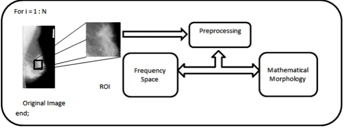
To perform performance testing on preprocessing algorithms, Figure 4 shows the steps through the investigation. First, the DDSM (Digital Database for Screening Mammography) database was selected, which is a public re-source for investigators. Primary support for this project was a grant from the Breast Cancer Research Program of the U.S. Army Medical Research and Materiel Command. The DDSM project is a collaborative effort in-volving co-p.i.s at the Massachusetts General Hospital (D. Kopans, R. Moore), the University of South Florida (K. Bowyer), and Sandia National Laboratories (P. Kegelmeyer). Additional cases from Washington University School of Medicine were provided by Peter E. Shile, MD, Assistant Professor of Radiology and Internal Medi-cine. Additional collaborating institutions include Wake Forest University School of Medicine (Departments of Medical Engineering and Radiology), Sacred Heart Hospital and ISMD, Incorporated. The primary purpose of the database is to facilitate sound research in the development of computer algorithms to aid in screening. Sec-ondary purposes of the database may include the development of algorithms to aid in the diagnosis and the de-velopment of teaching or training aids [14].

[image:4.595.144.488.581.711.2]

This database has 2479 cases on 41 volumes (Until October 2013), which are distributed on: 695 on 12 vo-lumes labeled as normal; 914 on 15 vovo-lumes labeled as cancer and 870 on 14 volumes classified as benign. The volumes are classified as: normal, cancer and benign; Normal cases are formed from a normal detection pre-vious exam (taken from a file) for a patient with a normal exam, at least, four years later. A normal detection exam is where more studies are no longer needed. Cancer cases are formed from detection exams in which are found cancer pathologies. Benign cases are formed from detection exams where suspicious pathologies are found, but they are not malignant. To perform the testing 60 cases were selected from 3 different volumes (cer_01, cancer_04, cancer_07) over 15 cancer volumes previously diagnosed (25 from can(cer_01, 14 from can-cer_04 and 21 from cancer_07). This is because the selected cases are those with abnormalities on microcalcifi-cations, checked by DDSM, which were processed by two filtering methods (morphology and frequency) to find the best optimal and provide the best result to its implementation on segmentation and classification algorithms.

(5)

2. Results

During the algorithms application shown on Figure 4, it was observed that on frequency space, specially low-pass filter, on Gaussian and Butterworth techniques, images do not show feature enhancement, which is not helpful to the extraction of knowledge and cannot be applied on future processes, therefore, it has been discarded from the investigation.

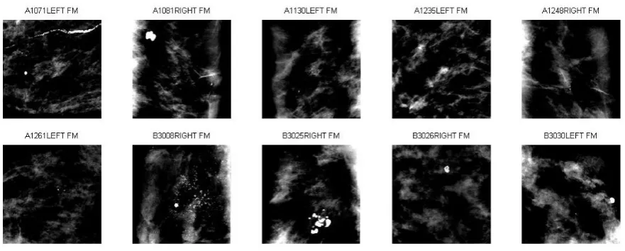
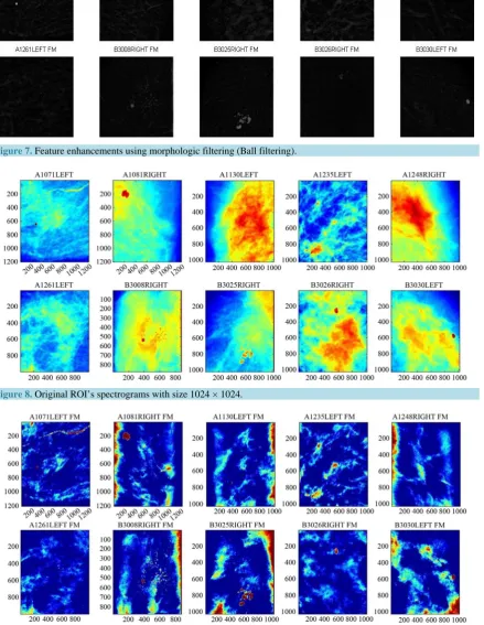
However, high-pass filter shows a clearly visible feature enhancement on frequency space. Figure 5 shows the original images taken from DDSM database. It can be seen that the filter on Figure 6, Gaussian technique, gets rid of tissue and enhances microcalcifications; however, the filtering does not remove all the tissue from the breast, which has the same gray-level than microcalcifications. This will bring identification class problems when clas-sification algorithms are applied. Figure 7 shows that morphology filtering, applying diamond technique, which enhances features on the image, being better than frequency space filtering, due to tissue elimination and en-hancing of possible microcalcifications. Then, every stage on this investigation is detailed.

[image:5.595.98.534.341.507.2]

On previous Figures 8-10 it could be seen the energy distribution on every ROI on its original format, fre-quency space filtering and morphology space filtering, unlike a histogram, they allow to observe or to watch the original context of images that show feature enhancement, that morphology preprocessing helps to get rid of tissue from breast. This tool also helps to compare between original and processed images, so it can be seen if filtering caused unwanted alterations to the image, taking out desired features that can be diagnosed as false po-sitives or false negatives in future processes. Finally a time test is shown on all algorithms made for frequency and morphology processing, to show how fast images can be processed on the search of microcalcifications. PC specifications are: CPU Intel i5 3450 3.1 GHz, 8 GB RAM 1600 MHz, HD 1 TB SATA-III, OS Windows 7 Ultimate

Figure 5. ROI’s of the original images (A1248, A1235, A1130, A1081, A1071, B3030, B3026, B3025, B3008, A1261).

[image:5.595.94.535.532.709.2]

(6)

[image:6.595.98.531.87.269.2]

Figure 7. Feature enhancements using morphologic filtering (Ball filtering).

Figure 8. Original ROI’s spectrograms with size 1024 × 1024.

[image:6.595.99.539.133.701.2]

(7)

[image:7.595.95.535.88.297.2]

Figure 10. Morphologic filtering spectrograms with size 1024 × 1024 (With ball filtring).

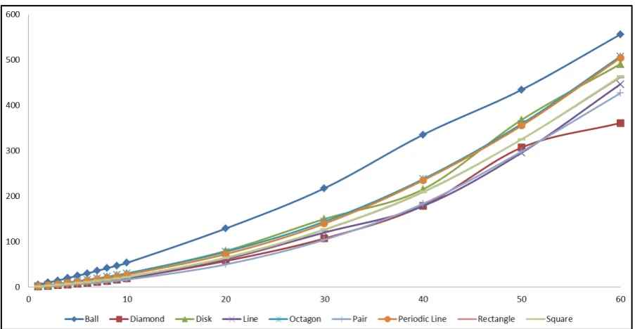
Table 1. Time graphic of frequency space preprocessing algorithms.

Images

Ball Diamond Disk Line Octagon Pair Periodic Line Rectangle Square

Time (s) Time (s) Time (s) Time (s) Time (s) Time (s) Time (s) Time (s) Time (s)

1 5 1.3 2.7 1.5 2.7 1 2.3 2 1.7

2 10 2.5 4.7 2.8 4.9 2.1 4.2 3.5 3.3

3 14.7 4 7.3 4.4 7.5 3.4 6.4 5.3 5

4 20 5.7 10.1 6.6 10.4 4.7 9 7.2 7

5 25.2 7.4 12.9 7.9 13.1 6.2 11.5 9.2 9

6 30.4 9.5 15.8 9.9 16.3 7.8 14.1 11.6 11.5

7 36.1 11.4 19 12.1 19.3 9.7 17.5 13.7 13.8

8 41.7 13.6 22.3 14.3 22.8 11.7 20.1 16.5 16.5

9 47.4 16.7 25.7 17.1 26.9 14.3 23.5 19.1 19.4

10 53.4 19 29.7 19.5 30.4 16.3 27.2 22.6 21.9

20 129 57.5 79.7 61.3 77.6 49.9 72.6 63.6 65

30 217.5 107.1 150 120.2 144.2 104.2 139.6 126.3 127

40 335.4 179 215.3 178.4 237.7 183.4 234.9 209.1 210.1

50 434.5 307.3 368.3 295.8 359.4 298.6 355.5 325.5 325.5

60 556.3 361.3 491.1 446.6 507.9 426.9 504.4 461.9 463.9

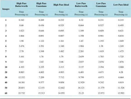
SP1 × 64. Table 1 and Table 2 represent the times for each of the filters used, each with their sub filtering in the frequency and space morphology.

[image:7.595.88.539.336.651.2]

(8)

[image:8.595.87.539.100.442.2]

Table 2. Time of morphologic space preprocessing algorithms.

Images

High Pass Butterworth

High Pass

Gaussiano High Pass Ideal

Low Pass Butterworth

Low Pass

Gaussiano Low Pass Ideal

Time Processing (s)

1 0.342 0.269 0.232 0.32 0.231 0.215

2 0.68 0.436 0.525 0.664 0.527 0.495

3 1.023 0.646 0.695 1.109 0.659 0.631

4 1.864 0.891 0.887 1.358 0.901 0.834

5 1.98 1.122 1.161 1.63 1.193 1.049

6 2.476 1.391 1.348 1.904 1.38 1.249

7 2.78 1.548 1.482 2.261 1.619 1.475

8 3.161 1.76 1.79 2.639 1.783 1.725

9 3.83 2.02 2.08 2.837 2.076 1.876

10 4.103 2.225 2.213 3.137 2.294 2.068

20 8.883 4.602 4.893 6.401 4.671 4.28

30 12.332 7.209 7.712 9.799 6.973 6.664

40 16.381 9.577 9.858 12.929 9.242 8.819

50 20.851 12.151 12.642 16.121 11.379 11.526

[image:8.595.86.540.150.704.2]

60 22.732 15.313 14.955 21.23 13.973 12.993

(9)

[image:9.595.87.539.82.316.2]

Figure 12.Time graphic of morphologic space preprocessing algorithms.

3. Discussion

Analyzing frequency space filtering, where its functionality is described, the higher the order, the closer it gets to its cutoff frequency. However, in real world testing, higher orders can be counterproductive for this investigation field, because there is a peak that overpasses cutoff frequency, allowing undesired frequencies to pass, the above makes that the filter shows some tissue as seen on Figure 6, and it can be checked on Figure 7, where accumulation of energy shows microcalcifications and tissue. This process is called resolution spectrogram window 1024 × 1024, which shows on similar colors the energy that represents microcalcifications and some energy accumulations on tissue, mixing up microcalcifications and tissue energies. Results can be seen on Fig- ure 9. Regarding morphology filtering there is a noticeable separation between tissue and microcalcifications, where a more homogeneous filtering can be seen. Even if the size of the window is modified, by half the size for example, image quality is affected and visualization of microcalcifications is influenced. However, if the size of the window is increased, more memory is required on the processing, and the spectrogram can be seen on Fig- ure 9 for morphology filtering. Finally, on every filter, lots of images were analyzed on time testing where the sample is 60 cases from 3 different volumes (cancer_01, cancer_04 and cancer_07), from 15 cancer volumes previously diagnosed (25 cases from cancer_01, 14 cases from cancer_04 and 21 cases from cancer_07). For frequency space filtering according to the graphic shown on Figure 10, times are low, meaning a fast processing, and every sub-filter is shown on the graphic and each sub-filter process from 1 image to 60 images, getting the lowest time: 13.973 seconds on Gaussian filter, and 22.732 seconds on high-pass Butterworth. Morphology fil-tering shows a slower processing: going from 363.1 to 556.3 seconds. The last point shows different times, al-though the frequency is faster than morphological space, and the morphological filters (Ball filtering) shows a significant result than frequency filters. That situation is supported on Figure 9 vs Figure 10. Finally, one of the benefits of image preprocessing is to enhance the characteristics of particular interest, which facilitates future processing steps (clustering, classification even neural networks).

References

[1] International Agency for Research Cancer (2013) http://www.iarc.fr/

[2] Instituto Nacional de Cancerología de México, Sistema de información de Cáncer (2013) http://www.infocancer.org.mx/contenidos.php?idcontenido=1

[3] Instituto Nacional de Estadística y Geografía (2014) http://www.inegi.org.mx/

(10)

http://www.cancer.gov/espanol/recursos/hojas-informativas/deteccion-diagnostico/mamografias.

[5] Quintanilla-Dominguez, J., Cortina-Januchs, M.G., Ojeda-Magana, B., Jevti, A., Vega-Corona, A. and Andina, D. (2010) Microcalcification Detection Applying Artificial Neural Networks and Mathematical morphology in Digital Mammograms. World Automation Congress.

[6] Guardado-Medina, R.O, Ojeda-Magaña, B., Quintanilla-Domínguez, J., Ruelas, R. and Andina, D. (2013) Quality of Microcalcification Segmentation in Mammograms by Clustering Algorithms. SOCO13, Salamanca, Spain.

[7] Ojeda-Magaña, B., Quintanilla-Dominguez, J., Ruelas, R. and Andina, D. (2009) Images Subsegmentation with the PFCM Clustering Algorithm. 7th IEEE International Conference on Industrial Informatics,23-26 June 2009,Cardiff, 499-505.

[8] Malar, E., Kandaswamy, A. and Gauthaam, M. (2013) Multiscale and Multilevel Wavelet Analysis of Mammogram Using Complex Neural Network. Springer International Publishing, Switzerland, 658-668.

[9] Chen, Z., Strange, H., Denton, E. and Zwiggelaar, R. (2014) Analysis of Mammographic Microcalcification Clusters Using Topological Features. Springer International Publishing, Switzerland, 620-627.

[10] Paradkar, S. and Spande, S. (2011) Intelligent Detection of Microcalcification from Digitized Mammograms. Sadhana,

36, 125-139.

[11] Gonzalez, R.C., Woods, R.E. and Eddins, S.L. (2004) Digital Images Processing Using Matlab. Pearson Education.

[12] Castleman, K.R. (1999) Digital Images Processing. Prentice Hall, Upper Saddle River.

[13] Gonzalez, R. C. and Woods, R.E. (1996) Tratamiento Digital de Imagines. Editorial Díaz de Santos, S.A.