Numerical Solution of Green’s Function for Solving Inhomogeneous Boundary Value Problems with Trigonometric Functions by New Technique

http://dx.doi.org/10.4236/am.2015.65072

Numerical Solution of Green’s Function for

Solving Inhomogeneous Boundary Value

Problems with Trigonometric Functions by

New Technique

Hamid Safdari, Yones Esmaeelzade Aghdam

Department of Mathematics, Shahid Rajaee Teacher Training University, Tehran, Iran Email: [email protected], [email protected]

Received 18 December 2014; accepted 6 May 2015; published 8 May 2015

Copyright © 2015 by authors and Scientific Research Publishing Inc.

This work is licensed under the Creative Commons Attribution International License (CC BY).

http://creativecommons.org/licenses/by/4.0/

Abstract

A numerical technique is presented for solving integration operator of Green’s function. The ap-proach is based on Hermite trigonometric scaling function on

[

0,2π

]

, which is constructed for Hermite interpolation. The operational matrices of derivative for trigonometric scaling function are presented and utilized to reduce the solution of the problem. One test problem is presented and errors plots show the efficiency of the proposed technique for the studied problem.

Keywords

Numerical Technique, Differential Equation, Green’s Function, Hermite Trigonometric Scaling, Wavelet, Error Estimate

1. Introduction

For concreteness, we assume that all functions are defined on the interval

[ ] [

a b, = 0,2π

]

, and we consider second-order ordinary differential operators Λ of the form

( )

( )

(

)

( )

( )

( )

( )

1 2 1 2

1 2 1 2

,

0, 0;

0, 0.

u p x u q x u x

u a u a

u b u b

δ ξ

α α α α

β β β β

_{Λ = ′}′_{+ = −}

 



 _{+ = + ≠}



 _{+ = + ≠}



(1)

where functions p x

( )

and q x

( )

are cntinuous for

[ ]

a b, , and δ

(

x−ξ

)

is dirac delta function. We look for a solution of 1 in the form

( )

_ab

( ) ( )

, d

u x =

_∫

G xξ f ξ ξ (2) where G a b: ,

[ ] [ ]

× a b, → is a suitable function, called the Green’s function of 1.

In most situations, it is difficult to obtain exact solution of the above integration. Hence, various approxi- mation methods have been proposed and studied. The purpose of the present paper is to develop a trigonometric Hermite wavelet approximation for the computing the Green’s function of the problem 2.

Recently, the arisen wavelet Galerkin method has demonstrated its advantages for the treatment of integral operators [1]-[5]. It is discovered in [6] that wavelet represents the singular integral operator. The development of fast methods for integral equations opens new perspectives. The methods like the fast multipole method [7]

and the panel clusteing [8] reduce the complexity largely. A difficulty of using wavelet for the representation of integral operators is that quadrature leads to potentially high cost with sparse matrix. This fact particularly en- courages us in efforts to devote to some appropriate wavelet bases to simplify the computation expense of the reoresentation matrix, which is importent to improve the wavelet method. Nowadays, the trigonometric inter- polant wavelet has arisen in the approximation of operators [9]-[11]. Quack [12] has constructed a multire- solution analysis (MRA) of nested subspace of trigonometric Hermite polynomials. The trigonometric Hermite interpolation enables a completely explicit description of the corresponding decomposition and reconstruction coefficients by means of some circular matrices. Chen [13] [14] presented the feasibility of trigonometric wave- let numerical methods for stokes problem and Hadamard integral equation.

The outline of this paper is as follows. In Section 2, we describe the trigonometric scaling function on

[

0,2π

]

, and in Section 3 we construct the operational matrix of derivative for these function. In Section 4, the proposed method is used to approximate the solution of the problem. As a result, a problem of integration of a matrix is obtained, where by calculating the Green’s function of this matrix we get to the solution of the problem. In Section 5, we report our computational results and demonstrate the accuracy of the proposed numerical schemes by presenting numerical examples. Section 6 ends this paper with a brief conclusion.

2. Trigonometric Scaling Function on

[

0,2π

]

In this section, we will give a brief introduction of Quak’s work on the construction of Hermite interpolatory trigonometric wavelets and their basic properties (see [12]). For all n∈, the Dirichlet kernel D xl

( )

and its

conjugate kernel D xl

( )

are defined as

( )

( )

_{( )}

_{( )}

1

1

1 sin

2 _{, 2π ;}

1 _cos

2sin

2 2

1 , 2π .

2

1

cos cos

2 _{2 , 2π ;}

sin _2sin

2

0, 2π .

l l

k

l l

k

l x

x x

D x kx

l x

x _l

x x

D x kx

x =

=

  ₊  

 _ _ 

 

 _∉

  

= + _{=   }

  



+ ∈

 

  ₋  ₊ 

   

 _{   }

 ∉



= =  

 

 _{ }



∈ 

∑

∑

Obviously, D x D x Tl

( )

, l

( )

∈ l is the linear space of trigonometric polynomials with degree not exceeding l.

The equally spaced nodes on the interval

[

0,2π

)

with a dyadic step are denoted by , π 2

j n j

n

t = , for any

{ }

0 0

j∈ = ∪ , and _{n=0,1, ,2} j+1_{−1, where}

{ }

0 = ∪ 0

, 0 is the set of all non-negative integers. Definition 1 (Scaling functions).(See[12].) For all j∈₀, the scaling functions 0

( )

,0

j x

ϕ , 1

( )

,0

j x

ϕ where

( )

(

)

, ,0 ,

s s

j n x j x xj n

ϕ =ϕ − for _{∀ =n 0,1, ,2} j+1_{−1 and s=0,1 are defined as}

( )

( )

( )

( )

(

)

1 1 2 1 0

,0 2 1

0

1 1

,0 2 1 2

1 _,

2

1 _{1 sin 2 .}

2 2

j

j

j j l

l

j

j j

x D x

x D x x

ϕ ϕ + + − + = + + =   = _ + _  

∑

Lemma 1 (See[12].) For j∈₀, we have

( )

( )

( )

(

(

)

)

2 2 2 0 2 ,0 1

1 2 2

,0

sin 2

1 _{, 2π ;}

2 _sin

2

1, 2π .

1 1 cos 2 cot , 2π ;

2 2

0, 2π .

j j j j j j x x x x x x x x x x ϕ ϕ + + +   ∉  _{ } =  _{ }     _∈   ₋   _∉    =    _∈ 

and their derivations are given by

( )

(

)

(

)

( )

( )

(

)

(

)

₍

₎

2 1

0 2 2 2

2 ,0

1

1

2 3 1

1 2

,0

sin 2 cot

sin 2

1 1 _{2 , 2π ;}

2 _sin 2 _sin

2 2

0 2π .

cos 2 1

1 _{1 sin 2 cot 2π ;}

2

2 _sin 2

2

1, 2π .

j j j j j j j j j j x x x x x x x x x _x x x x x x ϕ ϕ + + + + + + +       _{ }  − ∉  ′ =          _{   }  ∈   _{−  }  + _{ } ∉  ′_{= }           _∈ 

Theorem 2 (Interpolatory properties of the scaling functions).(See[12].) For j∈0, The following inter- polatory properties hold for each _{n k, =0,1, ,2} j+1₋₁

( )

(

( )

)

0 0

, , , , , , 0

j n xj k k n j n xj k

ϕ =δ ϕ ′= , (3)

( )

(

( )

)

1 1

, , 0, , , ,

j n xj k j n xj k k n

ϕ = ϕ ′=δ . (4) From above we can take wavelet functions 0

( )

,

j n x

ϕ , 1

( )

,

j n x

ϕ , _{n=0,1, ,2} j+1_{−1 as scaling functions. Then} we have

Definition 3 (Scaling functions space). For all j∈₀ define the wave space V as followsj

( )

( )

{

0 1 1

}

, ,

span , , 0,1, ,2j 1

j j n j n

V ₌ ϕ t ϕ t n₌ + ₋

As a first step of studying the spaces Vj, the following result identifies the trigonometric polynomials which

from alternative bases of these spaces. Theorem 4 For any j∈0, we have

( )

(

)

( )

(

)

{

1 1

}

span 1,cos , ,cos 2j 1 ,sin , ,sin 2j 1

j

consequently _{dim 2}j 2

j

V ₌ + _.

Definition 5 For any j∈0, the interpolation operator L mapping any real valued differentiable j 2π-

periodic function f into the space V is defined asj

( )

( )

2 11 0

( )

1

( )

T

, ,

0 j

j k j k k j k

k

f x L f x aϕ x bϕ x C

+₋

=

 + = Φ

 

∑

(5)

where ak = f x

( )

j k, bk = f x′

( )

j k, , and C and Φ are vectors with dimension 2j+2×1. The following properties of the operators Lj are therefore obvious:

1

2j j L T∈ +

( ) ( )

, , and

( ) ( )

,

( )

, ,

j j k j k j j k j k

L f x = f x L f ′ x = f x′ k∈

for all

j j

L f = f f V∈ .

Theorem 6 Let

( )

2 2π

f x ∈L , and its trigonometric wavelet approximation is L fj , then we have

( )

( )

( ) 2 2π 2 1 2 J j _L

f x L f x_{− ≤}C − + where C is a positive constant value.

Proof. See [12].

3. The Operational Matrix of Derivative

The differentiation of vector Φ in 5 can be expressed as [15]

Dφ ′

Φ = Φ

where Dφ is 2j+2×2j+2 operational matrix of derivative for trigonometric scaling function. Suppose

( )

(

)

2 1 1 0

( )

1

( )

, , , , ,

0 j

s s s

j m k m j k k m j k k

x a x b x

φ ϕ ϕ

+₋

=

′_{=  + }

 

∑

(6)

where _{m=0,1, ,2} j+1_{−1 and s=0,1. So the matrix D}

φ can be respresented as a block matrix as

0 0 1 1 A B D A B   =    

where _As _{and B}s _{are 2}j+1_×2j+1 _{matrices. The entries of matrices A}s _{and B}s _{may be finding by using 3}

( ) ( )

, ,

( )

, ,

( ) ( )

, ,

( )

,

s s s s s s

k m j k j m k m j k j m

A = a = φ ′ x B = b = φ ′′ x

where _A0 _{is a 2}j+1_×2j+1 _{zero matrix, A}1 _{is a 2}j+1_×2j+1 _{identity matrix. Using}

, ₂π

j m j

m

x = we get

( )

(

)

(

)

, , ,0 ,0 ,

π 2

s s s

j k j m j j j j m k

m k

x x

φ φ φ −

−

 

= _{ }=

  (7) Using Equation (7) and Bs =

( )

bk ms, =

(

φsj k,

( )

xj m,

)

′′=

(

φsj,0

(

xj m k, −

)

)

′′ s=0,1 we get

( ) ( )

(

)

(

)

(

)

(

)(

)

1 2

0 0 0 1

, ,0 ,

2 1 2 1

0 1

cos 2π

1 _{, ;}

2 sin π

2

1 2 1

1 _{, .}

6 2

j

j k m j j m k

p j p k m k k m m k

B b x

p p p

( ) ( ) (

)

1 1 1 1

, ,0 ,

cot π , ;

2

0, .

j k m j j m k

m k _{k m}

B b x

k m φ + − ₋  −  _≠  ′′   = = =    ₌  (9)

for _{k m, =0,1, ,2} j+1_−1.

4. Function Approximation

In this section, we give the concrete computational schemes for this integral Equation (2) with the Green’s function kernel. The discretization form of (2) is given in the following subsection.

By introducing a basis

{ }

φj k, for the subspace Vj, the coefficients vector G x

( )

j,ξ of the discrete

solution G x

( )

,ξ is defined by

( )

2 11 0

( )

1

( )

T

, ,

0 ,

j

j k j k k j k

k

GL G xξ aϕ x bϕ x C

+₋

=

 

=

∑

_ + _= Φ (10) where C is ₂j+2_{×1 unknown vector defined similar to (5). Using (2) we get}

( )

_ab j

( ) ( )

, d

u x =

_∫

L G xξ f ξ ξ (11) We tries to solve the above function by picking approximate values for N, WN i, and ξN i, . While only defined for the interval [−1, 1], this is a universal function actually, because we can convert the limits of inte- gration for any interval

[ ]

a b, to the Legendre-Gauss or G fN

( )

interval

[

−1,1

]

:

( )

( ) ( )

( )

1 1 , , , 1 , d , d

2 2 2 2 2

, .

2 2 2 2 2

b j a

N

N l N l N l N

l

u x L G x f

b a _{G x} b a b a _f b a b a

b a _{W G x} b a b a _f b a b a _{E G}

ξ ξ ξ

ξ ξ ξ

ξ ξ − = = −  − +   − +  = _ + _{ } + _     −  − ₊ +   − ₊ + ₊        

∫

∫

∑

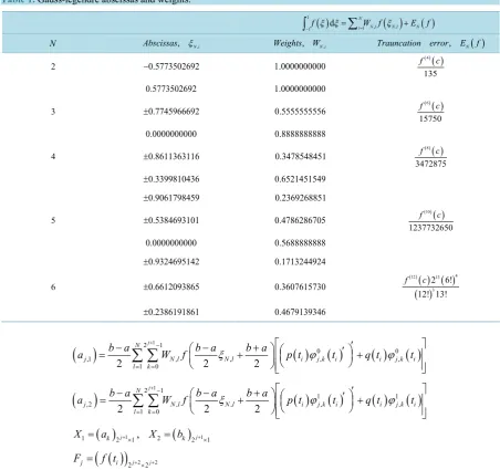
(12)

The abscissas ξN l, and weights WN l, to be used have been tabulated and are easily availabe;Table 1 gives the values up to six points. Also included in the table is the form of the error term E fN

( )

that corresponds to

( )

N

G f , and it can be used to determine the accuracy of the Gauss-Legendre integration formula. Applying Equation (10) in Equation (12) we have

( )

2 11 0

( )

1

( )

, , , ,

1 0

2 2 2

j

N

j N l N l k j k k j k

l k

b a b a b a

u x W f ξ aϕ x bϕ x E

+₋

= =

−  − + _{  }

= _ + _{ } + _+

 

∑ ∑

(13)

By substituting u x

( )

in (1), we have a linear system. Now for determining unknown coefficients ak and k

b , we choose collocation method With collocation points as

(

)

2

2 1

π _{; 0,1, ,2 1}

2 2

J

i J J

i b a i

t a i +

+ +

−

= + = = − (14)

( ) ( )

( ) ( )

(

)

( )

( )

( )

( )

1 2 1 2

1 2 1 2

,

0, 0;

0, 0.

i i i i i

u p t u t q t u t t

u a u a

u b u b

δ ξ

α α α α

β β β β

 _{ ′}′

Λ = + = −

 _{ }     + = + ≠   _{+ = + ≠}  (15)

Thus, we have system of linear equation A X Fj = j where Aj =

[

A A1 2

]

, 1 2 X X X   =  

 , N is the points of Gauss-Legendre, and

( )

, ₂j2 ₂j1, 1,2, 0,1, ,2 2 1

j s j s

A a + + s i

+ ×

[image:6.595.86.539.91.516.2]

Table 1. Gauss-legendre abscissas and weights.

( )

( )

( )

1

, , 1 1 d

N

N l N l N l

f ξ ξ ₌W f ξ E f

− =

∑

+

∫

N Abscissas, ξN i, Weights, WN i, Trauncation error, E fN( )

2 −0.5773502692 1.0000000000 ( )4( )

135

f c

0.5773502692 1.0000000000

3 ±0.7745966692 0.5555555556 ( )6( )

15750

f c

0.0000000000 0.8888888888

4 ±0.8611363116 0.3478548451 ( )8( )

3472875

f c

0.3399810436

± 0.6521451549

0.9061798459

± 0.2369268851

5 ±0.5384693101 0.4786286705 ( )10( )

1237732650

f c

0.0000000000 0.5688888888

0.9324695142

± 0.1713244924

6 ±0.6612093865 0.3607615730

( )_{( ) ( )} ( )

4 12 13

3

2 6! 12! 13!

f c

0.2386191861

± 0.4679139346

( )

2 1 1

( )

0

( )

( )

0

( )

,1 , , , ,

1 0

2 2 2

j

N

j N l N l i j k i i j k i

l k

b a b a b a

a W f ξ p t ϕ t q t ϕ t

+₋

= =

 ′ 

−  − +   ′

= _ + _{ } _ + 

 _ _

∑ ∑

( )

2 1 1

( )

1

( )

( )

1

( )

,2 , , , ,

1 0

2 2 2

j

N

j N l N l i j k i i j k i

l k

b a b a b a

a W f ξ p t ϕ t q t ϕ t

+₋

= =

 ′ 

−  − +   ′

= _ + _{  } _ + _

 

∑ ∑

( )

1

( )

1

1 k 2j 1, 2 k 2j 1

X = a +_× X = b +_×

( )

(

)

₂j2 ₂j2

j i

F = f t +_× +

So, the unknown function u xj

( )

can be found. Note that we find the function by MATLAB.

5. Numerical Example

To support our theoretical discussion, we applied the method presented in this paper to several examples. All the generalized Green’s function kernels in this numerical example are solved by trigonometric wavelet. Our me- thod compared with exact solution.

Example. Consider the inhomogeneous differential equation with the following coditions:

( )

( )

( )

sin 0 0

2π 0

u u x

u u

′′ + = 

 ₌



 ′ =



(16)

The exact solution is

( )

3sin

( )

sin 3

( )

sin 2

( )

cos

( )

8 8 4 2

x x x x

u x = − − − _{ }× x

descent method and results are shown inFigure 1. The relative errors between u x

( )

and u xj

( )

in absulote

error are given inTable 2 andTable 3, and different Gauss-Legendre Abscissas and Weights. It is easy to see that our error results are greatly small with low computing cost.

The above example states

1. Our numerical method is also efficient when the wave number J is very large, that is to say, the wave number J can hardly affect the convergence rate,

2. Our numerical method is very fast, for example, the run time is only 2.000 s as J = 8, for which the corresponding matrix Aj is 210×210.

6. Conclusion

The trigonometric scaling function is used to solve the Green’s function of an inhomogeneous differential equation. Some properties of trigonometric scaling function are presented and the operational matrices of derivative for trigonometric scaling function are utilized to reduce the solution of Green’s function to the solution of linear

[image:7.595.102.538.262.694.2]

(a) (b)

[image:7.595.86.540.505.717.2]

Figure 1. (a) Result for J = 1 and N = 3; (b) Result for J = 3 and N = 3.

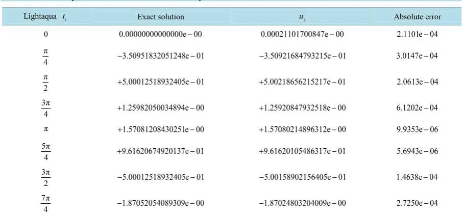
Table 2. Error analysis and numerical results of example for J = 1 and N = 3.

Lightaqua ti Exact solution uj Absolute error

0 0.00000000000000e 00− 0.00021101700847e 00− 2.1101e 04−

π

4 −3.50951832051248e 01− −3.50921684793215e 01− 3.0147e 04−

π

2 +5.00012518932405e 01− +5.00218656215217e 01− 2.0613e 04−

3π

4 +1.25982050034894e 00− +1.25920847932518e 00− 6.1202e 04−

π +1.57081208430251e 00− +1.57080214896312e 00− 9.9353e 06−

5π

4 +9.61620674920137e 01− +9.61620105486317e 01− 5.6943e 06−

3π

2 −5.00012518932405e 01− −5.00158902156405e 01− 1.4638e 04−

7π

[image:8.595.88.536.98.304.2]

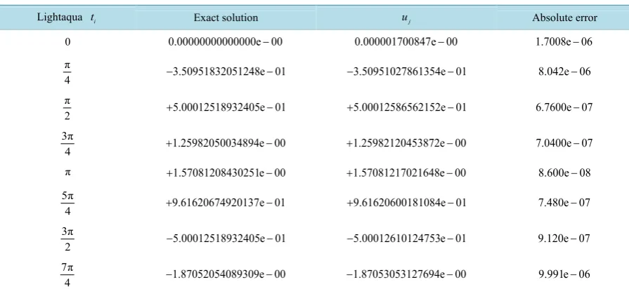
Table 3. Error analysis and numerical results of example for J = 3 and N = 3.

Lightaqua ti Exact solution uj Absolute error

0 0.00000000000000e 00− 0.000001700847e 00− 1.7008e 06−

π

4 −3.50951832051248e 01− −3.50951027861354e 01− 8.042e 06−

π

2 +5.00012518932405e 01− +5.00012586562152e 01− 6.7600e 07−

3π

4 +1.25982050034894e 00− +1.25982120453872e 00− 7.0400e 07−

π +_{1.57081208430251e 00}− +1.57081217021648e 00− 8.600e 08−

5π

4 +9.61620674920137e 01− +9.61620600181084e 01− 7.480e 07−

3π

2 −5.00012518932405e 01− −5.00012610124753e 01− 9.120e 07−

7π

4 −1.87052054089309e 00− −1.87053053127694e 00− 9.991e 06−

system of equations with sparse matrix of coefficients. Applications of the wavelets allow the creation of more effective and faster algorithms than the ordinary ones. Illustrative examples are included to demonstrate the vali- dity and applicability of the technique. The main advantage of this method is its simplicity and small com- putation costs.

Acknowledgements

The authors are very grateful to both refrees for carefully reading the paper and for comments and suggestions which have improved the paper.

References

[1] Chen, H. and Peng, S. (1999) A Quasi-Wavelet Algorithm for Second Boundary Integral Equations. Advances in Compu-tational Mathematics, 11, 355-375. http://dx.doi.org/10.1023/A:1018992413504

[2] Dahmen, W., Prossdorf, S. and Scheider, R. (1994) Wavelet Approximation Methods for Pseudodifferential Equations: I Stability and Convergence. Mathematische Zeitschrift, 215, 583-620. http://dx.doi.org/10.1007/BF02571732

[3] Huybrechs, D., Simoens, J. and Vandewalle, S. (2004) A Note on Wave Number Dependence of Wavelet Matrix Compression for Integral Equations with Oscillatory Kernel. Journal of Computational and Applied Mathematics,172, 233-246. http://dx.doi.org/10.1016/j.cam.2004.02.006

[4] Huybrechs, D. and Vandewalle, S. (2000) A Two-Dimensional Wavelet Packet Transform for Matrix Compression of Integral Equations with Highly Oscillatory Kernel. Journal of Computational and Applied Mathematics,197, 218-232. http://dx.doi.org/10.1016/j.cam.2005.11.001

[5] Von petersdorff, T. and Schwab, C. (1996) Wavelet Approximation for First Kind Integral Equations on Polygons.

Numerische Mathematik,74, 479-516. http://dx.doi.org/10.1007/s002110050226

[6] Beylkin, G., Coifman, R. and Rokhlin, V. (1991) Fast Wavelet Transforms and Numerical Algorithms. Communica-tions on Pure and Applied Mathematics,44, 141-183. http://dx.doi.org/10.1002/cpa.3160440202

[7] Greengard, L. and Rokhlin, V. (1987) A Fast Algorithm for Particle Simulation. Journal of Computational Physics,73, 325-348. http://dx.doi.org/10.1016/0021-9991(87)90140-9

[8] Hackbusch, W. and Nowak, Z.P. (1984) On the Fast Matrix Multiplication in the Boundary Element Method by Panel Clustering. Numerische Mathematik, 54, 463-491. http://dx.doi.org/10.1007/BF01396324

[9] Chui, C.K. and Mhaskar, H.N. (1993) On Trigonometric Wavelets. Constructive Approximation,9, 167-190. http://dx.doi.org/10.1007/BF01198002

[10] Prestin, J. (2001) Trigonometric Wavelets. In: Jain, P.K., et al., Eds., Wavelet and Allied Topics, Narosa Publishing House, New Delhi, 183-217.

Mathe-matics and InforMathe-matics, 14, 49-70.

[12] Quak, E. (1996) Trigonometric Wavelets for Hermite Interpolation. Mathematics of Computation, 683-722.

[13] Chen, W.S. and Lin, W. (1997) Hadamard Singular Integral Equations and Its Hermite Wavelet Methods. Proceedings of the 5th International Colloquiumon Finite Dimensional Complex Analysis,Beijing, 13-22.

[14] Chen, W.S. and Lin, W. (2002) Trigonometric Hermite Wavelet and Natural Integral Equations for Stockes Problem.

International Conference on Wavelet Analysis and Its Applications,Guangzhou, 73-86.