Trajectory Tracking Control of Robot Manipulators
Mukul Kumar Gupta
Assistant Professor, Department of EEI, University
of Petroleum & Energy Studies, Dehradun India
Arun Kumar Singh,
PhD. Assistant Professor, Department of Mechanical engineering, VNIT Nagpur,India
Kamal Bansal,
PhD. Professor, Department of EEIUniversity of Petroleum & Energy Studies, Dehradun
India
ABSTRACT
In this paper a simulink based approach is developed for trajectory tracking of robot manipulator. A robot manipulator is widely used in many industrial application.A robot manipulator moves the end effector to the configuration instructed by the user. The input from the main unit is transformed in to the desired configuration through forward kinematics. This configuration is sent to the robot controller to transform the configuration into joint angles. The simulink model is developed to provide basic block to model kinematics and trajectory tracking of robot manipulator. Availability of such library model of robot manipulator software, where the manipulator controller can be modelled using model library blocks and production can be automatically generated using existing code generators for simulink. In this the desired and the actual trajectory of the end effector under different conditions is shown with the help of MATLAB simulation.
Keywords
- Robot Dynamics, Cartesian space motion,Trajectory tracking
1.
INTRODUCTION
Model based development means that the main activity in the development process is designing a model of the system from the informal specification. Robot manipulators [1] [6] find many applications in many systems, for example spacecraft [2] industrial automation and life critical system. Simulink [8] is a high level model design tool is useful in many industrial application areas. Simulink [3] provides a wide range of library blocks for example arithmetic block, signal block, to name a few. By using subsystems it is possible to build a model of a large system in a hierarchical manner.
In this paper the objective is to show the applicability of model based [7] [8] development of robot software using simulink. In this a Cartesian space motion control for robot manipulator with revolute axes has been developed. The organisation of the paper as follows. Section 2 presents robot manipulator. Section 3 represents theory and simulation results. Section 4 concludes the conclusion and future work.
2.
ROBOT MANIPULATOR
A Robot Manipulators are composed of links connected by joints into a kinematic chain. Joints are typically rotary (revolute) or linear (prismatic).
Robot manipulator technology is constantly improving, by increasing efficiency and becoming more human interactive [9].The way to achieve the same performance in terms of speed, acceleration and operational load with less weight and increased human interactivity, is with flexible manipulator robots, due to their light weight structures and mechanical flexibility. A link parameter link length and link twist defines
the relative location of the two axes in space. A link parameter is link length and link twist. The link offset is the distance between two consecutive links along the axis of the joint. The joint angle is the rotation of one link with respect to the next about the joint axis. These four parameters together are called Denavit Hartenberg (D-H) parameters [4][5].The end effectors position can be controlled using either the joint angle or the link offset.
A revolute joint is like a hinge and allows relative rotation between two links. A prismatic joint allows a linear relative motion between two links each joint represents the interconnection between the links and the number of joints determine the degree of freedom of the manipulator.
A robot manipulator is composed of a set of links connected together by various joints. The joints can either be very simple (revolute joint or a prismatic joint) or complex (ball and socket joint). The difference between simple and complex joint is that, the simple joint has only a single degree-of-freedom of motion, the angle of rotation in the case of a revolute joint, and the amount of linear displacement in the case of a prismatic joint. In contrast, a ball and socket joint has two degrees-of-freedom one end of the robot manipulator called the base and the other end which is free is connected to an end effector. The difficulty of controlling a manipulator increases rapidly with the number of links. A manipulator having more than six links is referred to as a kinematic ally redundant manipulator.
The problems associated with motion of robot dynamics are forward kinematics, inverse kinematics, velocity kinematics, path planning and trajectory generation, vision dynamics, position control and force control
The forward kinematics problem is concerned with the relationship between the individual joints of the robot manipulator and the position and orientation of the tool or end-effector. The inverse problem of finding the joint variables in terms of the end effector position and orientation is the problem of inverse kinematics and it is in general more difficult than the forward kinematics problem. The velocity analysis is performed using a matrix quantity called the Jacobian. The dynamics equations of flexible manipulator robots are significantly more complex than those of rigid robots due to the link’s flexibility. Flexibility yields a robot model with infinite degrees of freedom, which must be truncated to a finite number. There are three principal objectives in the control of the flexible robot arms:
Point to point motion of the end-effector.
Trajectory tracking in the joint space (tracking of a desired angular trajectory).
Trajectory tracking in the operational space (tracking of a desired end-effector trajectory).
methodology, where the main objective is to determine on-line a desirable velocity profile along the path. One technique is to reduce all the undesired behaviour characteristics (such as vibration of the end-effector) of a flexible robot is to calculate the end-effector motion in such a way not to disturb the unstable zeros of the system.
Benosman and Le Vey [11] made a profound analysis about stable inversion of a SISO non-minimum phase linear system. Instead of searching for proper initial conditions associated to a given desired output, this approach, consists in a search for a proper output, associated to the desired initial conditions. This output is planned in a way that it is possible to cancel all the effects of the unstable zeros. After knowing the required output, it is possible to estimate the capable input to obtain the desired results. This methodology addresses the problem of planning a target tip trajectory leading to a finite smooth control torque that implies an exact reproduction of the computed trajectory by using a simple input-output inversion technique.
3.
TRACKING OF ROBOT
MANIPULATOR
For a robot manipulator the following two properties are mainly of interest
Property 1- While moving the end effector, no part of the robot manipulator should go inside an unsafe region.
Property 2- Eventually the end effector follows the desired trajectory within a certain specified error bound.
Regulation and Tracking
The task of every control problem can generally be divided into two categories:
Regulation (or stabilization) and tracking (or servoing). In the regulation problem, one is concerned with devising the control law such that the system states are driven to a desired final equilibrium point and stabilized around that point. In the tracking problem, one is faced with devising a controller (tracker) such that the system output tracks a given time varying trajectory. Some examples of regulation problems are: Temperature control of refrigerators, AC and DC voltage regulators, and joint position control robots. Examples of tracking problems can be found in tracking antennas, trajectory control of robots for performing specific tasks, and Control of mobile robots.
The formal definitions of the above control problems can be stated as follows [10]. Regulation Problem: Given a nonlinear dynamic system described by
= f(x, u, t)
Where x is the n x 1 state vector, u is the m x 1 input vector, and t is the time variable, find a control law u such that, starting from anywhere in a region in Ω c Rn, the state tends to zero as t → 0.
Similarly Tracking Problem: Given a nonlinear dynamic system and its output vector described by
= f(x, u, t)
y= h(x)
and a desired output trajectory yd(t), find a control law for the input u such that, starting from an initial state in a region Ω c Rn, the tracking error y ( t ) - yd(t) approaches to zero while the whole state x remains bounded
The control input u in the above definitions may be either called static if it depends on the measurements of the signals directly, or dynamic if it depends on the measurements through a set of differential equations. Tracking problems are Generally more difficult to solve than regulation problems. One reason is that, in the tracking problem, the controller has to drive the outputs close to the desired trajectories while maintaining stability of the whole state of the system. On the other hand, regulation problems can be regarded as special cases of tracking problems when the desired trajectory is constant with time.
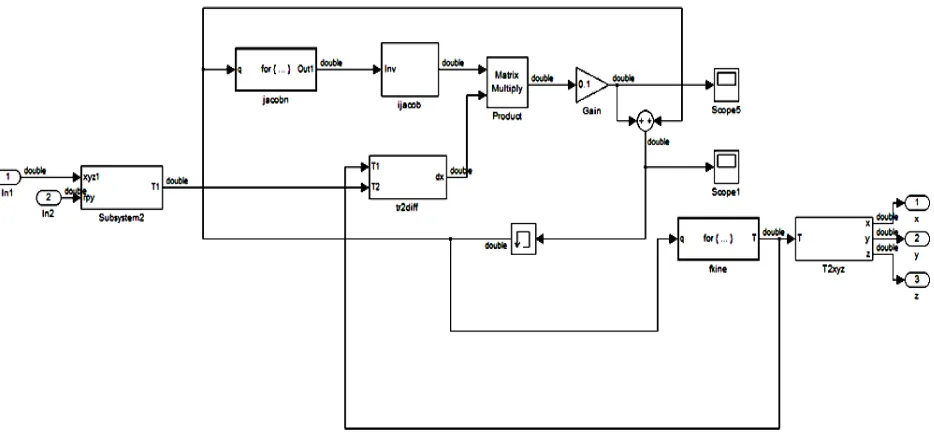
Fig. 1 Simulink model for trajectory control of robot manipulator
As a case study, the Cartesian space motion control of a robot manipulator is taken. The objective here is that the desired trajectory as given by the input should follow by the end effector of the manipulator. This can be obtained by two ways. Firstly, to perform the control in the joint space, the Cartesian space demand can be resolved to joint space through
inverse kinematics. Secondly, the error in Cartesian space can be used to resolve the error in the joint space via the inverse Jacobian. The second approach is adopted and models the controller using Model Rob Library blocks. The Simulink model is shown in Figure 1.
fig2 (a) x-y plot fig2 (a 1)
fig2(c ) fig2(c 1)
Fig. 2 {(a),(b),(c)} are the desired trajectory and {(a 1) (b1) (c 1)} are the actual trajectory
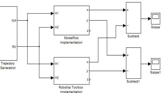
Few input trajectories were experimented, for example a constant point, a step function, and a circular trajectory. In Figure 2, we show how the end-effector tracks an arbitrary trajectory. Figure 2 shows the desired and the actual trajectory in the XY plane of circle, point and line respectively. It takes a few seconds before the end-effector reaches the desired trajectory. Afterwards, the end-effector follows the trajectory remaining in some error bound. The input trajectory is given to the manipulator models implemented using Model Rob Library and Robotics Toolbox [5]. Then, the difference
[image:4.595.166.439.393.551.2]between the x-coordinates and y-coordinates of the output trajectories for the two models with time is plotted. Figure 4, shows the difference between the x coordinates of the output trajectories of the two models with time. The figure shows that the error is of the order of 10-15 which provides confidence that the blocks in the Model Rob Library perform equivalent functionality with the corresponding blocks in the Robotics Toolbox.
Fig. 3 The conformance testing framework
[image:4.595.125.474.599.723.2]implementation of the functions. Two fixed-point are models for circular trajectory -one is with 8-bit data width, and the other is with 16-bit data width. The end effectors actual trajectory is compared for these fixed-point models with the end-effectors’ actual trajectory for the floating-point model. During simulation at different time points the graph is obtained which shows the difference between the actual x and y coordinates of the end-effectors in a fixed point model and the floating-point model. Figure 4 shows how the difference between the x-coordinates of the floating point. Simulink model and a fixed-point Simulink model varies with time (Figure 4(a) is for the 8-bit model and Figure 4(b) is for the 16-bit model). The plots show that for the Fig 4 The difference of the x coordinate of the trajectories of the end effector in floating point model and fixed point (a) 8 bit model and (b) 16 bit model.
4. CONCLUSION
In this paper, a simulink library is presented for modelling robot manipulator functionalities and how the trajectory will follow the end effector manipulator input and what is the difference between desired and the actual trajectories. This model based approach supports with only revolute joints and excludes the Prismatic joints. In future, the other variants like mobile robots, spherical and parallel robots can be developed. The library currently does not include blocks to perform robot dynamics. There are other variants of stationary robots, for example, cylindrical robot, spherical robot and parallel robot; and mobile robots, for example, wheel robot and legged robot, which Model Rob Library currently does not support. The main objective of this paper is to show that the model-based development approach can be successfully applied to the development of robot software and to motivate development of exhaustive library to cover all variants of robots.
5. REFERENCES
[1] J. H. Craig, Introduction to Robotics: Mechanics and Control. Addison-Wesley Longman Publishing Co., Inc., 1989.
[2] E. Papadopoulos and S. Dubowsky, “Coordinated manipulator/spacecraft motion control for space robotic systems,” in Proceedings of International Conference on Robotics and Automation, 1991, pp. 1696–1701
[3] The Math Works, “MathWorks TM - Simulink Reference”
http://www.mathworks.com/products/simulink/.
[4] Spong M.W. and VidyasagarM. Robot Dynamics and Control, John Wiley and Sons, 1989.
[5] P. I. Corke, “A robotics toolbox for MATLAB,” IEEE Robotics and Automation Magazine, vol. 3, no. 1, pp. 24–32, 1996.
[6] L. Sciavicco and B. Siciliano, Modelling and Control of Robot Manipulators. Springer 1995.
[7] C. Schlegel, T. Haler, A. Lotz, and A. Steck, “Robotic software systems: From code-driven to model-driven designs,” in Proc. 14th
Int. Conf. on Advanced Robotics, 2009
[8] N. Sharygina, J. Browne, F. Xie, R. Kurshan, and V. Levin, “Lessons learned from model checking a NASA robot controller,” Formal Methods in System Design, vol. 25, pp. 241–270, 2004.
[9] N.G. Hockstein, C.G. Gourin, R. A. Faust and D.J. Terris. A history of robots: from science fiction to surgical robotics, Journal of Robotic Surgery, 2007.
[10] J.J.E. Slotine and W. Li, "Applied Nonlinear Control," Prentice Hall, Englewood Cliffs, NJ, 1991
[11] M. Benosman and G. Le Vey. Stable inversion of siso non minimum phase linear systems through output planning: An experimental application to the one-link flexible manipulator. IEEE Transactions on Control Systems Technology, 11(4):5–29, July 2003.
[12] W. Khalil and E. Dombre. Modelling, Identification and control of robots. Hermes Penton Ltd, 2002.
[13] J. Hauser and R. Hindman. Manoeuvre regulation from trajectory tracking: feedback linearizable systems. In Proc. of third IFAC Symp. Of Nonlinear Control System Design, 1995.