Fuzzy Transshipment Problem
B. Abirami
Research Scholar,
Manonmaniam Sundaranar University,
D.G.Vaishnav College, Chennai, India
R. Sattanathan,
Associate Professor & Head Department of Mathematics,
D.G.Vaishnav College, Chennai, India
ABSTRACT
The fuzzy transportation problem in which available commodity frequently moves from one source to another source or destination before reaching its actual destination is called a fuzzy transshipment problem. To solve the fuzzy transshipment problem by linear programming problem using Simplex-type Algorithm by [1]. The advantage of this algorithm is that it does not use any artificial variables and it also reduces the iterations to get an optimum solution.
Mathematics Subject Classifications
90C08, 90C90.
Keywords
Fuzzy transshipment problem, Arsham-Khan’s Algorithm, Trapezoidal fuzzy numbers.
1.
INTRODUCTION
In a fuzzy transportation problem shipment of commodity takes place among sources and destinations. But instead of direct shipments to destinations, the commodity can be transported to a particular destination through one or more intermediated or fuzzy transshipment points. Each of these points in turn supply to other points. Thus, when the shipments pass from destination to destination and from source to source, fuzzy transshipments exists here. Such a problem cannot be solved as such by the usual fuzzy transportation algorithm, but slight modification is required before applying to the fuzzy transshipment problem. Transportation problem is solved by a simplex type algorithm by [1] to get an optimum solution. Later it was developed by [2] to solve the fuzzy transportation problem using triangular fuzzy numbers. In this paper it is further developed to solve the fuzzy transshipment problem by simplex type algorithm using trapezoidal fuzzy number to get an optimum solution.
Fuzzy transshipment problem is solved by a simplex type algorithm by [1] in two phases. In the first phase uses a basic variable iteration to develop a basic variable set which may or may not be feasible. The second phase uses a feasibility iteration to develop a feasible and optimum solution. Both the phases are used by the Gauss-Jordan pivoting method. The advantage of this method by [1] avoids artificial variables required by simplex method.
2.
PRELIMINARIES
In this section some basic definitions and arithmetic operations are reviewed by [6]:
Definition 1
: A fuzzy number 𝑎 is a trapezoidal fuzzy number denoted by (a1,a2,a3,a4) where a1,a2,a3 and a4 are real numbers and its membership function µã(x) is given below:µã(x) =
𝟎 𝐟𝐨𝐫 𝐱 ≤ 𝐚𝟏 𝐱−𝐚𝟏
𝐚𝟐−𝐚𝟏 𝐟𝐨𝐫 𝐚𝟏≤ 𝐱 ≤ 𝐚𝟐
𝟏 𝐟𝐨𝐫 𝐚𝟐 ≤ 𝐱 ≤ 𝐚𝟑 𝐚𝟒−𝐱
𝐚𝟒−𝐚𝟑 𝐟𝐨𝐫 𝐚𝟑≤ 𝐱 ≤ 𝐚𝟒
𝟎 𝐟𝐨𝐫 𝐱 ≥ 𝐚𝟒
Definition 2:
A special version of the linear ranking functions was proposed by [3] and [4] is as follows:ℛ (𝑎 ) = 𝑎
𝐿+𝑎𝑈
2
+ 1
2(β – α), where 𝑎 = (a
L
, aU , α ,β) be a trapezoidal number.
Definition 3:
We next define arithmetic on trapezoidal fuzzy numbers. Let 𝑎 = (aL, aU ,α ,β) and 𝑏 = (bL , bU ,γ ,θ) be two trapezoidal fuzzy numbers.Define, x>0, xЄR; x𝑎 = (xaL ,xaU , xα ,xβ) , x<0, xЄR; x𝑎 = (xaL ,xaU , -xβ ,-xα), 𝑎 ⊕𝑏 = (aL + bL ,aU + bU ,α+γ,β+θ).
𝑎 ⊗ 𝑏 = (a,b,c,d) where a = min(aLbL,aLθ,bLβ,βθ), b = min(aUbU,aUγ,αbU,αγ),c = max(aUbU,aUγ,αbU,αγ), d = max(aLbL,aLθ,bLβ,βθ).
3.
FUZZY TRANSSHIPMENT MODEL
Let us consider a fuzzy transportation problem with p sources Si , i= 1 to p and destinations Dj , j= 1 to q having fuzzy availability 𝑎𝑖 at initial source Si , i=1 to p and the fuzzy demand 𝑏𝑗 at initial destination Dj , j=1 to q. Let the following type of transshipment be allowed:
1. From a source to any another source. 2. From a destination to another destination. 3. From a destination to any source.
The number of sources and destinations in the transportation problem are p and q respectively. In transshipment problem we have p+q sources and destinations.
Thus the fuzzy transshipment problem may be written as:
Minimize 𝑍 = 𝑝+𝑞𝑖=1 𝑝+𝑞𝑗 =1,𝑗 ≠𝑖𝑐𝑖𝑗𝑥𝑗𝑖
Subject to 𝑝+𝑞𝑗 =1,𝑗 ≠𝑖𝑥𝑖𝑗 - 𝑝+𝑞𝑗 =1,𝑗 ≠𝑖𝑥𝑗𝑖 = 𝑎𝑖 , 𝑝+𝑞𝑖=1,𝑖≠𝑗𝑥𝑖𝑗 - 𝑝+𝑞𝑖=1,𝑖≠𝑗𝑥𝑗𝑖 = 𝑏𝑗 ,
where 𝑥𝑖𝑗 ≥ 0, i,j = 1,2,3…p+q, j≠i
The above formulation is a fuzzy transshipment model is reduced to transportation form by [5] as:
Minimize 𝑍 = 𝑝+𝑞𝑖=1 𝑝+𝑞𝑗 =1,𝑗 ≠𝑖𝑐𝑖𝑗𝑥𝑗𝑖
𝑝+𝑞𝑖=1 𝑥𝑖𝑗 =𝑃 , j = 1 to p
𝑝+𝑞𝑖=1 𝑥𝑖𝑗 = 𝑏𝑗 +𝑃 , j = p+1 to p+q
where 𝑥𝑖𝑗 ≥ 0, i,j = 1,2,3…p+q, j≠i
The balanced fuzzy transportation problem with
transshipment having p+q sources and p+q destinations. Add an amount of fuzzy buffer stock 𝑃 = 𝑝𝑖=1𝑎𝑖(or 𝑝+𝑞𝑗 =𝑝+1𝑏𝑗)
in the availability and demand corresponding to each source and destination nodes.
3.1
Algorithm to solve the Transshipment
problem
Step 1: Find the total fuzzy availability 𝑝𝑖=1𝑎𝑖 and the total
fuzzy demand 𝑝+𝑞𝑗 =𝑝+1𝑏𝑗. Let 𝑝𝑖=1𝑎𝑖 = (a,b,c,d) and
𝑏𝑗 𝑝+𝑞
𝑗 =𝑝+1 = (a',b',c',d'). Examine that the problem is balanced
or not. i.e. 𝑝𝑖=1𝑎𝑖 = 𝑝+𝑞𝑗 =𝑝+1𝑏𝑗 . If the problem is balanced
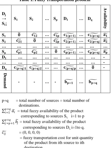
[image:2.595.309.547.98.443.2]then goes to step 2. The Fuzzy transportation problem table is shown in Table 1:
Table 1. Fuzzy Transportation problem
Dj
→ Si↓
S1 S2 … Sp D1 … Dq
Av
a
il
a
b
il
it
y
S1 𝟎 𝐜𝟏𝟐 … 𝐜𝟏𝐩 𝐜𝟏(𝐩+𝟏) … 𝐜𝟏(𝐩+𝐪) 𝐚𝟏
S2 𝐜𝟐𝟏 𝟎 … 𝐜𝟐𝐩 𝐜𝟐(𝐩+𝟏) … 𝐜𝟐(𝐩+𝐪) 𝐚𝟐
… … … … … … … … …
Sp 𝐜𝐩𝟏 𝐜𝐩𝟐 … 𝟎 𝐜𝐩(𝐩+𝟏) … 𝐜𝐩(𝐩+𝐪) 𝐚𝐩
D1 … … … … … … …
-… … … … … … … … -Dq 𝐜 𝐩+𝐪 𝟏 𝐜(𝐩+𝐪)𝟐 … … 𝐜 𝐩+𝐪 𝐩 … 𝟎
-De
m
a
n
d - - … - 𝐛𝐩+𝟏 … 𝐛𝐩+𝐪
p+q = total number of sources = total number of destinations.
𝑎𝑖 𝑝+𝑞
𝑖=1 = total fuzzy availability of the product
corresponding to sources Si, i=1 to p 𝑏𝑗
𝑝+𝑞
𝑗 =𝑝+1 = total fuzzy availability of the product
corresponding to sources Di, i=1to q. 𝑐𝑖𝑗 = (0, 0, 0, 0)
= fuzzy transportation cost for unit quantity of the product from ith source to ith destination.
𝑥 𝑖𝑗 = (aij, bij, cij, dij)
= the fuzzy quantity of the product that should be transported from the ith source to jth destination to minimize the total fuzzy transportation cost.
Step 2: A row in the table will be needed for each supply point and transshipment point, and a column will be needed for each demand point and transshipment point. Add an amount of fuzzy buffer stock 𝑃 = 𝑝𝑖=1𝑎𝑖(or 𝑝+𝑞𝑗 =𝑝+1𝑏𝑗) in the
availability and demand corresponding to each source and destination. Balanced fuzzy transportation problem with transshipment after adding an amount of fuzzy buffer stock
𝑃 = 𝑝𝑖=1𝑎𝑖(or 𝑝+𝑞𝑗 =𝑝+1𝑏𝑗) to each source and destination is
[image:2.595.50.287.305.620.2]shown in Table 2:
Table 2. Balanced Fuzzy Transportation problem
Dj
→ Si↓
S1 S2 … Sp D1 … Dq
Av
a
il
a
b
il
it
y
S1 𝟎 𝐜𝟏𝟐 … 𝐜𝟏𝐩 𝐜𝟏(𝐩+𝟏) … 𝐜𝟏(𝐩+𝐪) 𝐚𝟏
⊕ 𝐏
S2 𝐜𝟐𝟏 𝟎 … 𝐜𝟐𝐩 𝐜𝟐(𝐩+𝟏) … 𝐜𝟐(𝐩+𝐪) 𝐚𝟐
⊕ 𝐏
… … … … … … … … …
Sp 𝐜𝐩𝟏 𝐜𝐩𝟐 … 𝟎 𝐜𝐩(𝐩+𝟏) … 𝐜𝐩(𝐩+𝐪) 𝐚𝐏
⊕ 𝐏
D1 … … … … … … … 𝐏
… … … … … … … … -Dq 𝐜 𝐩+𝐪 𝟏 𝐜(𝐩+𝐪)𝟐 … … 𝐜 𝐩+𝐪 𝐩 … 𝟎 𝐏
De
m
a
n
d - - …
-𝐛 𝐩+𝟏
⊕ 𝐏
…
𝐛𝐩+𝐪
⊕ 𝐏
𝑃 = (p1, p2, p3, p4) is the fuzzy buffer stock.
Step 3: Using Arsham-Khan’s Simplex Tableau [1] to get an optimum basic feasible solution for the given fuzzy transshipment problem.
3.2 Numerical Example
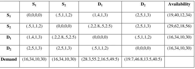
Consider the following fuzzy transshipment problem involving two sources and two destinations. The fuzzy availability of the sources S1 and S2 are (3,6,2,4) and (13,28,8,26) respectively. The fuzzy demand values of destinations D1 and D2 are (12.3,21.2,6.5,19.5) and (3.7,12.8,3.5,10.5) respectively. The fuzzy transportation cost for unit quantity of the product between different sources and destinations are summarized as in Table 3. Find the fuzzy optimal shipping plan for this fuzzy transportation problem with transshipment.
Step 1: Total fuzzy availability = (16,34,10,30) and total fuzzy demand = (16,34,10,30). So it is a balanced fuzzy transportation problem, if not balanced it.
Step 2: The balanced fuzzy transportation problem with transshipment having four sources and four destinations after adding an amount of fuzzy buffer stock P = (16,34,10,30) to each source and destination nodes in Table 4.
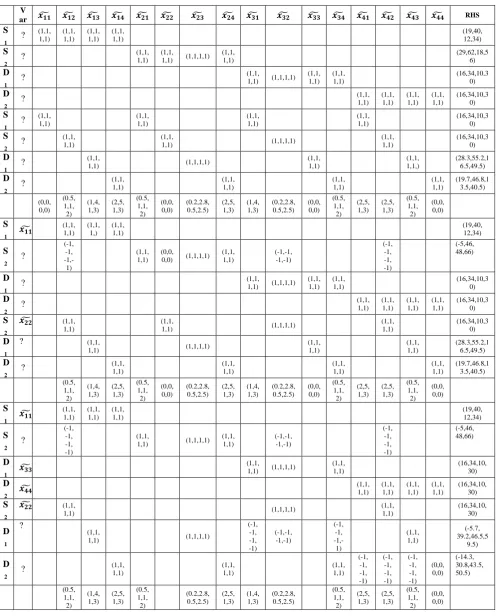
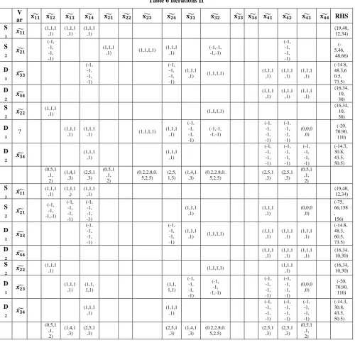
Step 4: Construct Arsham- Khan’s Simplex Tableau as shown in Table 5, Table 6.Right hand side values are positive as shown in Table 8; therefore we get an optimum solution. Hence Arsham-Khan’s simplex table by [1] is complete.
Table 3. Summary of fuzzy transportation cost for unit quantity of the product between different sources and destinations
S1 S2 D1 D2 Availability
S1 (0,0,0,0) (.5,1,1,2) (1,4,1,3) (2,5,1,3) (3,6,2,4)
S2 (.5,1,1,2) (0,0,0,0) (.2,2.8,.5,2.5) (2,5,1,3) (13,28,8,26)
D1 (1,4,1,3) (.2,2.8,.5,2.5) (0,0,0,0) (.5,1,1,2) -
D2 (2,5,1,3) (2,5,1,3) (.5,1,1,2) (0,0,0,0) -
Demand - - (12.3,21.2,6.5,19,5) (3.7,12.8,3.5,10.5)
Table 4. Balanced fuzzy transshipment problem
S1 S2 D1 D2 Availability
S1 (0,0,0,0) (.5,1,1,2) (1,4,1,3) (2,5,1,3) (19,40,12,34)
S2 (.5,1,1,2) (0,0,0,0) (.2,2.8,.5,2.5) (2,5,1,3) (29,62,18,56)
D1 (1,4,1,3) (.2,2.8,.5,2.5) (0,0,0,0) (.5,1,1,2) (16,34,10,30)
D2 (2,5,1,3) (2,5,1,3) (.5,1,1,2) (0,0,0,0) (16,34,10,30)
[image:3.595.104.497.322.462.2]Table 5. Iterations I
V
ar 𝒙𝟏𝟏 𝒙𝟏𝟐 𝒙𝟏𝟑 𝒙𝟏𝟒 𝒙𝟐𝟏 𝒙𝟐𝟐 𝒙𝟐𝟑 𝒙𝟐𝟒 𝒙𝟑𝟏 𝒙𝟑𝟐 𝒙𝟑𝟑 𝒙𝟑𝟒 𝒙𝟒𝟏 𝒙𝟒𝟐 𝒙𝟒𝟑 𝒙𝟒𝟒 RHS
S
1
? (1,1,1,1) (1,1,1,1) (1,1,1,1) (1,1,1,1) (19,40, 12,34)
S
2
? (1,1,1,1) (1,1,1,1) (1,1,1,1) (1,1,
1,1)
(29,62,18,5 6)
D
1
? (1,1,1,1) (1,1,1,1) (1,1,
1,1) (1,1, 1,1) (16,34,10,3 0) D 2
? (1,1,1,1) (1,1,1,1) (1,1,1,1) (1,1,1,1) (16,34,10,30)
S
1
? (1,1,1,1) (1,1,1,1) (1,1,1,1) (1,1,1,1) (16,34,10,30)
S
2
? (1,1,1,1) (1,1,1,1) (1,1,1,1) (1,1,
1,1)
(16,34,10,3 0)
D
1
? (1,1,1,1) (1,1,1,1) (1,1,
1,1) (1,1, 1,1,) (28.3,55.2,1 6.5,49.5) D 2
? (1,1,1,1) (1,1,1,1) (1,1,1,1) (1,1,1,1) (19.7,46.8,13.5,40.5)
(0,0, 0,0) (0.5, 1,1, 2) (1,4, 1,3) (2,5, 1,3) (0.5, 1,1, 2) (0,0, 0,0) (0.2,2.8, 0.5,2.5) (2,5, 1,3) (1,4, 1,3) (0.2,2.8, 0.5,2.5) (0,0, 0,0) (0.5, 1,1, 2) (2,5, 1,3) (2,5, 1,3) (0.5, 1,1, 2) (0,0, 0,0) S 1
𝒙𝟏𝟏 (1,1,1,1) (1,1,1,) (1,1,1,1) (19,40, 12,34)
S 2 ? (-1, -1, -1,-1) (1,1, 1,1) (0,0,
0,0) (1,1,1,1)
(1,1, 1,1) (-1,-1, -1,-1) (-1, -1, -1, -1) (-5,46, 48,66) D 1
? (1,1,1,1) (1,1,1,1) (1,1,
1,1) (1,1, 1,1) (16,34,10,3 0) D 2
? (1,1,1,1) (1,1,1,1) (1,1,1,1) (1,1,1,1) (16,34,10,30)
S
2
𝒙𝟐𝟐 (1,1,
1,1)
(1,1,
1,1) (1,1,1,1)
(1,1, 1,1) (16,34,10,3 0) D 1
? (1,1,
1,1) (1,1,1,1)
(1,1, 1,1) (1,1, 1,1) (28.3,55.2,1 6.5,49.5) D 2
? (1,1,1,1) (1,1,1,1) (1,1,1,1) (1,1,1,1) (19.7,46.8,13.5,40.5)
(0.5, 1,1, 2) (1,4, 1,3) (2,5, 1,3) (0.5, 1,1, 2) (0,0, 0,0) (0.2,2.8, 0.5,2.5) (2,5, 1,3) (1,4, 1,3) (0.2,2.8, 0.5,2.5) (0,0, 0,0) (0.5, 1,1, 2) (2,5, 1,3) (2,5, 1,3) (0.5, 1,1, 2) (0,0, 0,0) S 1
𝒙𝟏𝟏 (1,1,1,1) (1,1,1,1) (1,1,1,1) (19,40, 12,34)
S 2 ? (-1, -1, -1, -1) (1,1, 1,1) (1,1,1,1) (1,1, 1,1) (-1,-1, -1,-1) (-1, -1, -1, -1) (-5,46, 48,66) D 1
𝒙𝟑𝟑 (1,1,1,1) (1,1,1,1)
(1,1, 1,1) (16,34,10, 30) D 2
𝒙𝟒𝟒 (1,1,1,1)
(1,1, 1,1) (1,1, 1,1) (1,1, 1,1) (16,34,10, 30) S 2
𝒙𝟐𝟐 (1,1,
1,1) (1,1,1,1) (1,1, 1,1) (16,34,10, 30) D 1 ? (1,1, 1,1) (1,1,1,1) (-1, -1, -1, -1) (-1,-1, -1,-1) (-1, -1, -1,-1) (1,1, 1,1) (-5.7, 39.2,46.5,5 9.5) D 2
? (1,1,1,1) (1,1, 1,1) (1,1, 1,1)
Table 6 Iterations II
V
ar 𝐱𝟏𝟏 𝐱𝟏𝟐 𝐱𝟏𝟑 𝐱𝟏𝟒 𝐱𝟐𝟏 𝐱 𝟐𝟐 𝐱 𝟐𝟑 𝐱 𝟐𝟒 𝐱 𝟑𝟏 𝐱 𝟑𝟐 𝐱 𝐱𝟑𝟑 𝐱𝟑𝟒 𝟒𝟏 𝐱 𝟒𝟐 𝐱 𝐱𝟒𝟑 𝟒𝟒 RHS S
1
𝒙𝟏𝟏 (1,1,1,1)
(1,1,1 ,1) (1,1,1 ,1) (19,40, 12,34) S 2 𝒙𝟐𝟏 (-1, -1, -1, -1) (1,1,1
,1) (1,1,1,1)
(1,1,1 ,1) (-1,-1, -1,-1) (-1, -1, -1, -1) (-5,46, 48,66) D 1 𝒙𝟑𝟑 (-1, -1, -1, -1) (-1, -1, -1, -1) (1,1,1
,1) (1,1,1,1)
(1,1,1 ,1) (1,1,1 ,1) (1,1,1 ,1) (-14.8, 48.3,6 0.5, 73.5) D 2
𝒙𝟒𝟒 (1,1,1,1)
(1,1,1 ,1) (1,1,1 ,1) (16,34, 10, 30) S 2
𝒙𝟐𝟐 (1,1,1,1) (1,1,1,1)
(16,34, 10, 30)
D
1
? (1,1,1,1) (1,1,1,1) (1,1,1,1) (1,1,1
,1) (-1, -1, -1, -1) (-1,-1, -1,-1) (-1, -1, -1, -1) (-1, -1, -1, -1) (0,0,0 ,0) (-20, 70,90, 110) D 2
𝒙𝟑𝟒 (1,1,1,1) (1,1,1,1)
(-1, -1, -1, -1) (-1, -1, -1, -1) (-1, -1, -1, -1) (-14.3, 30.8, 43.5, 50.5) (0.5,1 ,1, 2) (1,4,1 ,3) (2,5,1 ,3) (0.5,1 ,1, 2) (0.2,2.8,0. 5,2.5) (2,5, 1,3) (1,4,1 ,3) (0.2,2.8,0. 5,2.5) (2,5,1 ,3) (2,5,1 ,3) (0.5,1 ,1, 2) S 1
𝒙𝟏𝟏 (1,1,1,1)
(1,1,1 ,) (1,1,1 ,1) (19,40, 12,34) S 2 𝒙𝟐𝟏 (-1, -1, -1,-1) (-1, -1, -1, -1) (-1, -1, -1, -1) (1,1,1 ,1) (1,1,1 ,1) (0,0,0 ,0) (-75, 66,158 , 156) D 1 𝒙𝟑𝟑 (-1, -1, -1, -1) (-1, -1, -1, -1) (1,1,1
,1) (1,1,1,1)
(1,1,1 ,1) (1,1,1 ,1) (1,1,1 ,1) (-14.8, 48.3, 60.5, 73.5) D 2
𝒙𝟒𝟒 (1,1,1,1)
(1,1,1 ,1) (1,1,1 ,1) (16,34, 10,30) S 2
𝒙𝟐𝟐 (1,1,1,1) (1,1,1,1) (1,1,1
,1)
(16,34, 10,30)
D
1
𝒙𝟐𝟑 (1,1,1,1)
(1,1, 1,1) (1,1, 1,1) (-1, -1, -1, -1) (-1, -1, -1,-1) (-1, -1, -1, -1) (-1, -1, -1, -1) (0,0,0 ,0) (-20, 70,90, 110) D
2 𝒙𝟑𝟒
[image:5.595.49.550.77.570.2](1,1,1 ,1) (1,1,1 ,1) (-1, -1, -1, -1) (-1, -1, -1, -1) (-1, -1, -1, -1) (-14.3, 30.8, 43.5, 50.5) (0.5,1 ,1, 2) (1,4,1 ,3) (2,5,1 ,3) (2,5,1 ,3) (1,4,1 ,3) (0.2,2.8,0. 5,2.5) (2,5,1 ,3) (2,5,1 ,3) (0.5,1 ,1, 2)
Table 7. Iterations III
V
ar 𝐱 𝒙𝟏𝟏 𝟏𝟐 𝒙𝟏𝟑 𝒙𝟏𝟒 𝒙𝟐𝟏 𝐱 𝐱𝟐𝟐 𝐱𝟐𝟑 𝟐𝟒 𝐱 𝟑𝟏 𝐱 𝟑𝟐 𝐱 𝐱𝟑𝟑 𝐱𝟑𝟒 𝟒𝟏 𝐱 𝟒𝟐 𝐱 𝟒𝟑 𝐱 𝟒𝟒 RHS S
1
𝒙𝟏𝟏 (1,1,1,1)
(0,0,0, 0) (0,0,0, 0) (1,1,1, 1) (1,1,1, 1) (-56, 106, 170, 190) S 2 𝒙𝟐𝟏 (-1, -1, -1,-1) (1,1, 1,1) (1,1, 1,1) (1,1,1, 1) (-1, -1, -1,-1) (0,0,0, 0) (-66, 75,156, 158) D 1 𝒙𝟑𝟑 (-1, -1, -1, -1) (-1, -1, -1, -1) (1,1,1,
1) (1,1,1,1)
(1,1,1, 1) (1,1,1, 1) (1,1,1, 1) (-14.8, 48.3, 60.5, 73.5) D 2
𝒙𝟒𝟒 (1,1,1,1)
(1,1,1, 1) (1,1,1, 1) (16,34, 10,30) S 2
𝒙𝟐𝟐 (1,1,1,1)
(-1, -1, -1,-1) (-1, -1, -1,-1) (1,1,
1,1) (1,1,1,1)
D
1
𝒙𝟐𝟑 (1,1, 1,1)
(1,1, 1,1)
(1,1, 1,1)
(-1, -1, -1, -1)
(-1, -1, -1,-1)
(-1, -1, -1, -1)
(-1, -1, -1, -1)
(0,0,0, 0)
(-20, 70,90,
110)
D
2
𝒙𝟑𝟒 (1,1,1,1) (1,1,1,1)
(-1, -1, -1, -1)
(-1, -1, -1, -1)
(-1, -1, -1, -1)
(-14.3, 30.8, 43.5, 50.5) (0.5,1,
1, 2)
(1,4,1, 3)
(2,5,1, 3)
(2,5,1, 3)
(1,4,1, 3)
(0.2,2.8,0.5, 2.5)
(2,5,1, 3)
(2,5,1, 3)
[image:6.595.81.517.203.430.2](0.5,1, 1, 2)
Table 8. The optimum Fuzzy Transshipment Table
S1 S2 D1 D2 Availability
S1
(0,0,0,0)
[-56,106,170,190]
(0.5,1,1,2)
[-66,75,156,158]
(1,4,1,3) (2,5,1,3) (19,40,12,34)
S2 (0.5,1,1,2)
(0,0,0,0)
[-59,100,168,186]
(0.2,2.8,0.5,2.5)
[-20,70,90,110]
(2,5,1,3) (29,62,18,56)
D1 (1,4,1,3) (0.2,2.8,0.5,2.5)
(0,0,0,0)
[-14.8,48.3,60.5,73.5]
(0.5,1,1,2)
[-14.3,30.8,43.5,52.5]
(16,34,10,30)
D2 (2,5,1,3) (2,5,1,3) (0.5,1,1,2)
(0,0,0,0)
[16,34,10,30]
(16,34,10,30)
Demand (16,34,10,30) (16,34,10,30) (28.3,55.2,16.5,49.5) (19.7,46.8,13.5,40.5)
It is shown in Table 8 thatthe optimum fuzzy transportation cost is [-111.6, 140.8, 451.5, 617.25]
Defuzzified fuzzy transportation cost is 56.0375.
4.
CONCLUSION
The proposed algorithm yields an optimum solution of the fuzzy transshipment problem. The main advantage of the proposed method is solved manually, without using artificial variables which is required by the simplex method also it reduces number of iterations.
5.
REFERENCES
[1] H.Arsham and A.B.Kahn, A simplex-type algorithm for general transportation problems: An alternative to Stepping-stone, Journal of Operational Research Society, 40(1989), 581-590.
[2] A.Nagoor Gani, A.Edward Samuel and D.Anuradha,
Simplex Type Algorithm for solving Fuzzy
Transportation Problem, Tamsui Oxford Journal of Information and Mathematical Sciences 27(1)(2011) 89-98.
[3] N.Mahdavi-Amiri and S.H.Nasseri, Duality results and a dual simplex method for linear programming problems with trapezoidal fuzzy variables, Fuzzy Sets and Systems 158(2007) 1961-1978.
[4] R.R.Yager, A procedure for ordering fuzzy subsets of the unit interval, Inform.Sci 24(1981) 143-161.
[5] Amit Kumar, Amarpreet Kaur, Anila Gupta, Fuzzy Linear Programming Approach for Solving Fuzzy Transportation Problems with Transshipment Math Model Algor(2011)10:163-180.
[6] R.E.Belman and L.A.Zadeh, Decision making in a fuzzy
Environment, Management science,17(1970),B141-