Two Second Order Nonlinear Extended Kalman Particle Filter Algorithms

http://dx.doi.org/10.4236/ojs.2015.54027

Two Second-Order Nonlinear Extended

Kalman Particle Filter Algorithms

Hongxiang Dai, Li Zou

Department of Statistics, Jinan University, Guangzhou, China Email: [email protected]

Received 9 April 2015; accepted 29 May 2015; published 2 June 2015

Copyright © 2015 by authors and Scientific Research Publishing Inc.

This work is licensed under the Creative Commons Attribution International License (CC BY).

http://creativecommons.org/licenses/by/4.0/

Abstract

In algorithms of nonlinear Kalman filter, the so-called extended Kalman filter algorithm actually uses first-order Taylor expansion approach to transform a nonlinear system into a linear system. It is obvious that this algorithm will bring some systematic deviations because of ignoring nonli-nearity of the system. This paper presents two extended Kalman filter algorithms for nonlinear systems, called second-order nonlinear Kalman particle filter algorithms, by means of second-order Taylor expansion and linearization approximation, and correspondingly two recursive formulas are derived. A simulation example is given to illustrate the effectiveness of two algorithms. It is shown that the extended Kalman particle filter algorithm based on second-order Taylor expansion has a more satisfactory performance in reducing systematic deviations and running time in com-parison with the extended Kalman filter algorithm and the other second-order nonlinear Kalman particle filter algorithm.

Keywords

Kalman Particle Filter, Nonlinear System, Taylor Expansion, Linearization Approximation

1. Introduction

It is well known that the theory of Kalman filter has been widely used in many scientific fields. Particularly, the linear Kalman filter algorithm has received a great deal of attention due to its effectiveness in estimating the state of an underlying linear system in [1]. However, it has been recognized that nonlinearity and disturbance exist in many practical linear systems, which leads to considering nonlinear Kalman filter algorithms of nonli-near state-space systems in [2].

of the system equation, a sub-optimal state estimate for a nonlinear state-space system can be given in [3]. In order to reduce error in the estimation of the system state and improve the precision of EKF, various modified algorithms have been established. For example, Uhlmann et al. [4] give a kind of unscented Kalman filter (UKF) algorithm for nonlinear systems. This algorithm has the same calculation capacity as the EKF algorithm and re-duces error in linearizing nonlinear model. Merwe et al.[5] present an algorithm called central difference Kal-man filter (CDKF) and deduce its recursive formula. This algorithm is easier to realize than EKF, because it does not need to compute Jacobi matrices. But UKF and CDKF are not suitable for non-Gaussian state-space systems. If a state-space model is nonlinear and noise distributions are non-Gaussian, particle filters (PFs) or sequential Monte Carlo (SMC) methods provide an effective algorithm to deal with this case [6]. A combination of EKF and PF leads to extended Kalman particle filter (EKPF) algorithm, where EKF algorithm updates the sampling particles and the particles approximate the filtering distributions. The EKPF algorithm has been ap-plied to neural networks in [7], and the results show that the algorithm is superior to other basic particle filter algorithms. Although these algorithms have some advantages in effectiveness and calculation speed for most of nonlinear state-space models, sometimes we need some more accurate Kalman filter algorithms to estimate the state of nonlinear systems.

To this end, this paper will give two Kalman particle filter algorithms for nonlinear state-space models. One is based on second-order Taylor expansion of structural functions of nonlinear system (SEKPF), the other, denoted by SLEKPF, uses a linearization method to approximate the quadratic of second order Taylor expansion of struc- tural functions. Accordingly, recursive formulas of the above nonlinear Kalman filter algorithms are derived. A simulation example is given to compare EKPF with SEKPF and SLEKPF. It can be seen from running time and root mean square error of the state estimation that they have similar calculation capacity, but SLEKPF is supe-rior to EKPF and SEKPE in accuracy of state estimation.

2. Nonlinear Kalman Filter

2.1. Extended Nonlinear Kalman Filter

For a nonlinear state-space model, the extended Kalman filter is a frequently used method to estimate the system state. The key point of this algorithm is to use first-order Taylor expansion to approximate the structural func-tions of the model. More precisely, a general nonlinear discrete-time state-space model is given as follows:

( )

( ) ( )

1 1,

, 0.

t t t

t t t t

v

y a x h w t

ξ ξ

ξ

+ = Φ + +

= + + ≥

where the system state ξ_t and the noise v_t+₁ are r-dimensional, whiled the observation value yt and the

noise w_t are n-dimensional. Moreover, the following assumptions are satisfied:

(

)

(

)(

)

( )

(

)

( )

(

)

(

)

(

)

( )

T

1 0 1 0 1 1 0 1 1 0 1 0

T T

1 1 1

T T T

ˆ _, ˆ ˆ

0, , 0,

cov , 0, cov , 0, 0, .

t t t t t t

i j i j i j

E E P

E v E v v Q E w E w w R

v v w w E w v i j

ξ δ ξ ξ ξ ξ ξ

+ + + = − − = = = = = = = = ≠ ， ,

If Φ ⋅

( )

is a twice continuously differentiable function and h

( )

⋅ is a continuously differentiable function, then we use Taylor expansion of Φ ⋅

( )

and h

( )

⋅ to approximate these function. In this case, the nonlinear state-space model (1) can be described approximately as a linear model. Let

δ

t=

(

y yt, t−₁,,y x x₀, ,t t−₁,,x₀

)

denote the information flow, namely, the observed data obtained through date t−1 be summarized. Suppose that the initial value of the state vector ξ₁ of the state-space model (1) is normally distributed and the distur- bances v_t and w_t are normal. Then

ξ δ

t t and , 1

t t t t x y ξ δ₋    

  obey normal distributions as well. Since h has continuous first-order partial derivatives and Φ has continuous second-order partial derivative functions, it is not difficult to linearize the nonlinear state-space model (1) with the help of Taylor expansion. Now define

( )

₍

₎

1 ˆ

, 1

t t t

t t h

h t t

ξ ξ

ξ

ξ

− = ∂ _′ = − ∂ ,

( )

_{( )}

ˆ ,

t t t

t t t t ξ ξ

ξ

ξ

₌ ∂Φ _′ = Φ ∂ ,

( )

_{( )}

2 ˆ ,

t t t

t T t t t t ξ ξ ξ

ξ ξ ₌

∂ Φ

′′ = Φ

mated by linear model can be used as follows:

( )

( )

(

)

( )

( )

(

)

(

)

1 1

1 1

ˆ _, ˆ _,

ˆ _{, 1} ˆ _.

t t t t t t t

t t t t t t t t

t t v

y a x h h t t w

ξ ξ ξ ξ

ξ ξ ξ

+ +

− −

′

= Φ + Φ − +

′

= + + − − +

Proposition 2.1 If the discrete time linear system (3) satisfies (2), and the disturbances v_t and w_t are

in-dependent and obey normal distributions, then we have (1) state estimates

( )

+1

ˆ ˆ

t t t t ξ = Φ ξ , and

(2) mean square error matrix of system.

( )

(

( )

)

T

1 , ,

t t t t

P₊ = Φ′ t t P Φ′ t t +Q.

The proof of Proposition 2.1 can be found in [8]. Although the EKF algorithm is simple and effective for some nonlinear state-space models, it is likely to lead to sub-optimal state estimate due to removing higher-order terms of structural equations in Taylor expansion. In what follows, two modified nonlinear Kalman filter algo-rithms will be given for the purpose of reducing errors of the state estimation.

2.2. Second-Order Nonlinear Kalman Filter Algorithms

In the extended nonlinear Kalman filter algorithm, an application of first-order Taylor expansion on Φ results in a linear state equation. This linearization approximation will cause some errors and instability of algorithm in some sense. It is natural to use second-order Taylor expansion to approximate Φ.

Proposition 2.2 Under the same conditions as Proposition 2.1, if Φ is twice continuously differentiable and

h is continuously differentiable, then the nonlinear state-space model (1) has the following nonlinear Kalman filter algorithm, namely,

(1) state estimates are given by

( )

(

( )

)

+1

1

ˆ ˆ _{tr ,}

2

t t t t t t Pt t

ξ = Φ ξ + Φ′′

and

(2) mean square error matrix of system

( )

( )

_T

(

)

2

1

1

, , tr

2

t t t t t t

P₊ = Φ′ t t P _Φ′ t t _ + _ Φ′′P _ +Q.

Proof: To guarantee normality of y_t, we take the linear part of Taylor expansion of h. Thus we have

( )

( )

ˆ 1

(

, 1

)

(

ˆ 1

)

t t t t t t t t

y =a x +h ξ ₋ +h t t′ − ξ ξ− ₋ +w .

Note that , 1

t t t t

x y

ξ δ−

 

 

  is normal, so is

ξ δ

t t. By reference [8],

(

) (

)

_T

(

)

1

(

( )

( )

)

1 1 1 1

ˆ ˆ _{, 1 , 1 , 1} ˆ

t t

t t t t Pt t h t t h t t Pt t h t t R y a x h t t

ξ =ξ ₋ + ₋ ′ − _ ′ − ₋ ′ − + _− − − ξ ₋ ,

(

)

(

(

)

)

_T

(

)

1

(

)

T

1 1 , 1 , 1 1 , 1 , 1 1

t t t t t t t t t t

P P P h t t h t t P h t t R h t t P

−

− − ′  ′ − ′  ′ −

= − − _ − − + _ − .

An application of Taylor expansion to Φ gives that

( )

( )

(

) (

)

T

( )

(

)

1 1

1

ˆ _, ˆ ˆ _, ˆ

2

t t t t t t t t t t t t t t t t vt

Taking conditional expectations on both sides of (5), the state estimates are given by

(

1

)

( )

(

( )

)

1

1

ˆ ˆ _{tr ,}

2

t t

t t E t t t t Pt t

ξ₊ = ξ δ₊ = Φ ξ + Φ′′

where we have applied the following fact that, if Z has mean µ and variance Σ, then

(

)

( )

(

)

(

( )

)

T T

2

T T

Var 2 tr 4 .

E Z AZ A tr A

Z AZ A A A

µ µ

µ µ

= + Σ

= Σ + Σ

；

On the other hand, the residual is expressed as

( )

(

) (

)

T

( )

(

)

(

( )

)

1 1

1 1

ˆ _, ˆ ˆ _, ˆ _{tr ,}

2 2

t t t t t t t t t t t t t t t t t t Pt t vt

ξ₊ −ξ₊ = Φ′ ξ ξ− + ξ ξ− Φ′′ ξ ξ− − Φ′′ +

Thus the mean square error matrix of system is

(

)(

)

T

( )

( )

_T

(

( )

)

2

1 1 1 1

1

1

ˆ ˆ _{, , tr ,}

2

t t t t

t t t t t t

P+ =E ξ+ −ξ+ ξ+ −ξ+ = Φ′ t t P Φ′ t t  + _ Φ′′ t t P _ +Q.

It should be pointed out that the above nonlinear Kalman filter algorithm needs to calculate Hessian matrix of Φ. Such an approximation, on one hand, increases running time, on the other hand, cannot guarantee normality of ξ_t, so it will influence on multi-step predictions of the state. In next proposition, we will apply linearization approximation to the quadratic in (5) and deduce corresponding recursive formula of nonlinear Kalman filter algorithm.

Proposition 2.3 Under the same conditions as Proposition 2.2 we have the following nonlinear Kalman filter

algorithm for the nonlinear system (1): (1) state estimates are

( ) (

)

T

( )

(

)

1 1 1

1

ˆ ˆ ˆ ˆ _, ˆ ˆ _{, 1}

2

t t t t t t t t t t t t t t t

ξ₊ = Φ ξ + ξ ₋ −ξ Φ′′ ξ ₋ −ξ ≥ .

and

(2) mean square error matrix of system state is

( )

(

)

T

( )

( )

(

)

T

( )

T

1 , ˆ ˆ 1 , , ˆ ˆ 1 , , 1.

t t t t t t t t t t t t

P₊ = Φ_ ′ t t −

ξ

−

ξ

₋ Φ′′ t t _P _Φ′ t t −

ξ

−

ξ

₋ Φ′′ t t _ +Q t≥

   

Proof: Firstly, a second-order Taylor expansion of Φ gives that

( )

( )

(

) (

)

T

( )

(

)

1 1

1

ˆ _, ˆ ˆ _, ˆ

2

t t t t t t t t t t t t t t t t vt

ξ₊ = Φ ξ + Φ′ ξ ξ− + ξ ξ− Φ′′ ξ ξ− + ₊ ,

Applying first-order Taylor expansion to

(

)

( )

(

)

T

ˆ _, ˆ

t t t t t t t t

ξ ξ− Φ′′ ξ ξ− , we have

(

)

T

( )

(

) (

)

T

( )

(

) (

)

T

( )

(

)

1 1 1 1

ˆ _, ˆ ˆ ˆ _, ˆ ˆ ₂ ˆ ˆ _, ˆ

t t t t t t t t t t t t t t t t t t t t t t t t t t t

ξ ξ− Φ′′ ξ ξ− = ξ ₋ −ξ Φ′′ ξ ₋ −ξ + ξ ₋ −ξ Φ′′ ξ ξ− ₋

This also implies that

( )

( )

(

) (

)

( )

(

) (

)

( )

(

)

( )

( )

(

)

( )

(

) (

)

( )

(

)

T T

1 1 -1 -1 1

T T

1

1 1 1

1

ˆ _, ˆ ˆ ˆ _, ˆ ˆ ˆ ˆ _, ˆ

2

1

ˆ _, ˆ ˆ _, ˆ ˆ ˆ _, ˆ ˆ _.

2

t t t t t t t t t t t t t t t t t t t t t t

t t

t t t t t t t t t t t t t t t t

t t t t t t v

t t t t t t v

ξ ξ ξ ξ ξ ξ ξ ξ ξ ξ ξ ξ

ξ ξ ξ ξ ξ ξ ξ ξ ξ

+ − +

+

− − −

′ ′′ ′′

= Φ + Φ − + − Φ − + − Φ − +

 _{′ ′′}  _′′

= Φ + Φ_ − − Φ _ − + − Φ − +

 

It is not hard to get that

(

)

( ) (

)

T

( )

(

)

1

1 1 1

1

ˆ ˆ ˆ ˆ _, ˆ ˆ

2

t t

t t E t t t t t t t t t t t t

Moreover, the mean square error matrix of system is given by

( )

(

)

T

( )

( )

(

)

T

( )

T

1 , ˆ ˆ 1 , , ˆ ˆ 1 ,

t t t t t t t t t t t t

P₊ = Φ_ ′ t t −

ξ

−

ξ

₋ Φ′′ t t _P _Φ′ t t −

ξ

−

ξ

₋ Φ′′ t t _ +Q

   

Note that in this nonlinear filter algorithm, we have applied first-order Taylor expansion to deal with the qua- dratic

(

ξ ξt− ˆt t

)

TΦ′′

( )

t t,

(

ξ ξt− ˆt t

)

, thus

ξ δ

t+1 t still obeys normal distribution in this case. This also implies

that this algorithm can give multi-step predictions of the system state.

2.3. Extended Particle Filter Algorithm

The extended particle filter (EKPF) algorithm was initially given by Freitas in [9], under the framework of EKPF algorithm. This algorithm applies recursive formula of EKF to update each particle and will get an ap-proximate posterior probability density of ξ_t. By the posterior probability distribution, new samples from the distribution are represented by a set of particles. Each particle has a weight assigned to it that represents the probability of that particle being sampled from the probability density function. In the resampling step, the par-ticles with negligible weights are replaced by new parpar-ticles in the proximity of the parpar-ticles with higher weights. EKPF, SEKPF and SLEKPF algorithm are as follows [10]:

(1) Set initial value k=0;

(2) Draw N particles from prior distribution (important distribution);

(3) Apply recursive formulas of EKF, SEKF, and SLEKF to update sampling particles; (4) Update weights;

(5) Normalize weights; (6) Resample,

(7) k= +k 1,

(8) If the number of particles is enough, the procedure stops.

3. Two Simulation Examples

To compare EKPF with SEKPF and SLEKPF algorithms, we use single variable non-stable growth model in [11] and gas phase reversible reaction model in [12].

Example 3.1 Consider the following nonlinear state-space model:

(

)

1 2 1

2

25

0.5 8cos 1.2 ,

1 . 20

t

t t t

t

t

t t

t w

y v

ξ

ξ ξ

ξ ξ

+ = + ₊ + + +

= +

where the initial state ξ₀ is normally distributed with mean 0 and variance 2, the noise w_t has Gamma distri-bution with mean 0.5 and variance 0.5, and the noise v_t is also normally distributed with mean 0 and variance 1. The number of particles is 200 and the whole time is 30 seconds, and we have 100 independent experiments. The aim is to compute the average value of the particles. A formal formula is as follows [13]:

1 1

ˆ N j

t t

j N

ξ ξ

=

=

∑

,

where N is number of particles.

The root-mean-square error is defined as:

(

)

2 1

1 _ˆ

RMSE T

k k k

T = ξ ξ

=

∑

−

where T is the whole time.

[image:6.595.204.425.81.285.2]

Figure 1.State estimation curve of three algorithms.

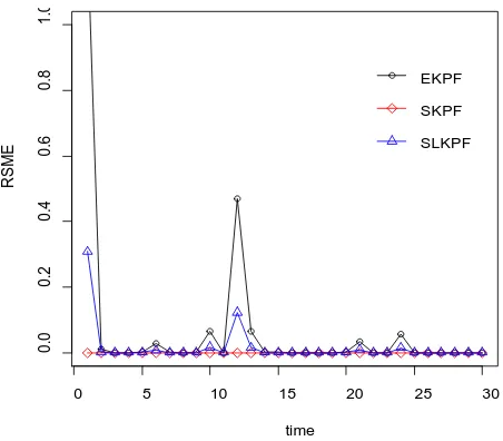
Figure 2. Root mean square error curves of three algorithms.

the EKPF algorithm has the worst performance in estimating the system state. The reason lies in no considera-tion of higher-order Taylor expansion term. Means and variances of 100 root-mean-square errors and running time for the above particle filter algorithms are given inTable 1. The results show that the SEKPF algorithm have the minimum root-mean-square error in average. Although in three algorithms, the running time of EKPF is the shortest. We can conclude that the SEKPF and SLEKPF algorithms can effectively increase the precision of state estimations.

Example 3.2 Consider the following nonlinear state-space model:

[ ]

,1

1,1 ,1

,1

,1

1,2 ,2 ,2

,1

, 1 0.032

0.016

, 1 0.032

1,1 .

t

t t

t

t

t t t

t

t t t

x

x w

x

x

x x w

x

y x v

+

+

= +

+

= + +

+

= +

where the noises w1,t and w2,t obey Gamma distributions with mean 0.5 and variance 0.5, the noise vt is normally

time

E

s

ti

m

a

te

d

S

ta

te

0 5 10 15 20 25 30

-2

0

-1

0

0

10

20

30

observed value true value

EKPF SKPF SLKPF

time

R

S

M

E

0 5 10 15 20 25 30

0

.0

0

.2

0

.4

0

.6

0

.8

1

.0

EKPF

SKPF

[image:6.595.202.428.307.505.2]

distributed with mean 0 and variance 0.1. We take vector x_{1 0} =

[ ]

3,1 and covariance matrix _{1 0} 36 10 01

P = ×   

 .

[image:7.595.91.542.360.710.2]

The number of particles is 200. The whole time is 30 seconds. We have 100 independent experiments.

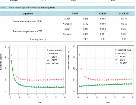
Table 2 gives means and variances of 100 independent root-mean-square errors and running time for three algorithms. Figure 3shows state estimations of (6) obtained from three Kalman particle filter algorithms. From these, we have similar conclusions to Example 3.1. Therefore, two second-order nonlinear Kalman particle filter algorithms proposed in this paper are superior to the EKPF algorithm in the precision of state estimations.

4. Conclusion

In many practical state-space models, the observation equations are linear, but the state equations are nonlinear; sometimes the disturbances are non-Gaussian [14]. For such a state-space model, we need to give an appropriate Kalman filter algorithm to estimate the system state. In this paper, we have proposed two nonlinear Kalman fil-ter algorithms, and corresponding recursive formulas have been derived. One is based on second-order Taylor Table 1. Root-mean-square errors and running time of three kinds of algorithms.

Algorithms

Root-mean-square error

Running time (s)

Mean Variance

EKPF 0.295 0.309 1.87

SKEPF 0.179 0.152 1.98

SLEKPF 0.190 0.240 2.03

Table 2. Root-mean-square errors and running time.

Algorithm EKPF SEKPF SLEKPF

Root-mean-squareerrors of X1

Mean 0.035 0.008 0.016

Variance 0.142 0.005 0.072

Root-mean-square error of X2

Mean 0.064 0.062 0.063

Variance 0.005 0.001 0.001

Running time (s) 2.87 2.98 3.05

Figure 3. State estimate.

time

E

s

ti

m

at

ed S

tat

e(

X

1)

0 5 10 15 20 25 30

0

10

20

30

40

observed value true value

EKPF SKPF SLKPF

time

E

s

ti

m

at

ed S

tat

e(

X

2)

0 5 10 15 20 25 30

0

10

20

30

40

observed value true value

expansion of the state equation, and the other uses a linearization approach to approximate the quadratic of second-order Taylor expansion of the state equation. In order to improve the precision of state estimation, we have combined the above nonlinear Kalman filter algorithms with particle filter and given two nonlinear Kalman particle filter algorithms. Through two examples, we compare the two nonlinear Kalman particle filter algo-rithms with the extended Kalman particle filter algorithm. The simulation results show that our second-order Kalman particle filter algorithms are superior to the extended Kalman particle filter algorithm. On one hand, two nonlinear Kalman particle filter algorithms have stronger calculation capacity than the extended Kalman filter particle algorithm; on the other hand, they can effectively improve state estimations.

References

[1] Daum. F. (2005) Nonlinear Filters: Beyond the Kalman Filter. IEEE A&E Systems Magazine, 20, 57-69. http://dx.doi.org/10.1109/MAES.2005.1499276

[2] Doucet, A. and Johansen, A. (2011) A Tutorial on Particle Filtering and Smoothing: Fifteen Years Later. In: Crisan, D. and Rozovskii, B., Eds., The Oxford Handbook of Nonlinear Filtering, Oxford University Press, New York, 656-704. [3] Cappe, O., Godsill, S.J. and Moulines, E. (2007) An Overview of Existing Methods and Recent Advances in

Sequen-tial Monte Carlo. Proceedings of the IEEE, 95, 899-924. http://dx.doi.org/10.1109/JPROC.2007.893250

[4] Gao, Y., Gao, S. and Wu, J. (2014) Fading-Memory Square-Root Unscented Particle Filter Algorithm and Its Applica-tion in Integrated NavigaApplica-tion System. Journal of Chinese Inertial Technology, 22, 777-781.

[5] Qian, Z. and Qi, Y. (2012) A SLAM Algorithm Based on an Iterated Central Difference Particle Filter. Journal of Harbin Engineering University, 33, 355-360.

[6] Zhu, Z. (2012) Particle Filter Algorithm and Application. Science Press, Beijing.

[7] Wang, F. and Guo, Q. (2010) Neural Network Training Based on Extended Kalman Particle Filter. Computer Engi-neering & Science, 32, 48:50.

[8] Zhao, L. (2012) Nonlinear Kalman Filter Theory. National Defense Industry Press, Beijing.

[9] Julier, S.J., Uhlmann, J.K. and Durrant-Whyten, H.F. (2000) A New Approach for the Nonlinear Transformation of Means and Covariance in Filters and Estimators. IEEE Transactions on Automatic Control, 45, 477-482.

http://dx.doi.org/10.1109/9.847726

[10] Wang, F. and Zhao, Q. (2008) A New Particles to Solve the Problem of Nonlinear Filter Algorithm. Chinese Journal of Computers, 31, 346-352.

[11] Liu, X., Tao, Z., Jin, Y. and Yang, Y. (2010) A Novel Multiple Model Particle Filter Algorithm Based on Particle Op-timization. Acta Electronica Sinica, 38, 301-305.

[12] Kolas, S., Foss, B.A. and Schei, T.S. (2009) Constrained Nonlinear State Estimation-Based on the UKF Approach.

Computers & Chemical Engineering, 33, 1386-1401. http://dx.doi.org/10.1016/j.compchemeng.2009.01.012

[13] Wang, F., Lu, M., Zhao, Q. and Yuan, Z. (2014) Particle Filtering Algorithm. Chinese Journal of Computers, 37, 1679-1693.