Some possibilities exist to design the parameters of motion screws. All the respective theories are based on the buckling stress calculation. Some of the so called construction schools use classical methods of design and calculations (Bolek & Kochman 1989), others use the buckling stress conversion to pressure stress by means of buckling coefficients (Orlov 1979) or by using special formulas, e.g. by American Society (Faires 1955; Oberk et al. 2000; Marghitu 2001), or Johnson’s formula (Marghitu 2001). All the methods mentioned are based on it-erations, requiring too many calculation opit-erations, especially in the case of the inexperienced designer. In designing the motion screws, the effective length change during the operation has to be considered inducing kinetic energy changes of the screw as well as the inaccuracies in both the nut bearing and the point of action.
Motion screw
Motion screws are often connected with the ancient ingenious man, Archimedes. But for his basic theses and postulates, the current sciences would not exist. Archimedes also practiced his theoretical knowledge of physics by constructing. He gave foundations to many scientific disciplines and is considered by many as the greatest inventor of all ages.
Besides many his accomplishments which brought him imperishable glory, Archimedes is a creator of
the water pump based on the motion screw as the operational element. His revolutionary device has been used to pump out water from under the ship deck and for the water transport in agriculture.
Another milestone in history is the life work of an Italian painter, artist, mathematician and inventor, Leonardo da Vinci. He started to use motion screws to lift weight. His system of jack is still in use nowa-days, as well as the screw based presses.
The golden age of motion screws dates back to the eighteenth century when the so called industrial revolution changed the world. Motion screws were frequently used by English inventors and construc-tors such as John Wilkinson together with Henry Maudsley. The most gifted inventor of that era was undoubtedly Joseph Whitworth who formed the foundations of the thread accurate cutting, thread measuring, and finally its construction. Leonardo’s jack construction was improved by using the ball bearing whose mass production started in many countries towards the end of the nineteen century. The motion screws were then already part of every day living. These were met by railroad and steam-boat travelers. Motion screws are the essential parts of floodgates in English channels connecting the northern and southern parts of the country.
Later, they became indispensable in many indus-trial branches, sciences and medicine. Their function is not limited only to lifting weight but also to trans-forming the circular motion to the advance motion
Utilisation of the method of stress limit for designing the
motion screw dimensions
D. Herák
1, J. Karanský
2, R. Chotěborský
31
Department of mechanics and engineering,
2Department of technological equipments of building,
3Department of material and engineering technology, Faculty of Engineering, Czech University
of Life Sciences in Prague, Prague, Czech Republic
Abstract: A design of the motion screw using the method of stress limit is described. Further general formulas are induced to design such kind of screws, applied to an example of 11500 (EN ISO E295) steel made screw, strained by static operational force. Safety equations to prevent screw drift and their diagrams are integrated parts of the article.
and contrariwise. As sad fact remains that motion screws were used to improve the construction of artillery grenade direction finders, leading to higher numbers of human casualties during wars.
MATERIAL AND METHODS
The motion screws with threads are used to kinetic energy transmission at lower rotation number of screw or nut. The motion screw and its nut are mu-tually housed with one degree of freedom. It means a case of buckling at motion.
Theory of allowable stress limit
As early as in 18th century, Leonhard Euler dis-covered and formulated a formula which described maximal value of axial force; such force was trans-ferred by slender bars without the loss of stabil-ity. The described theory was evolved by solving a simple differential equation of the deflection curve, loaded by axial force, rising a bending moment. In the case of such calculation, bars are considered as ideal, meaning a bar is straight, homogenous, and without internal preload. Maximal value of tension originated during a load is called the critical load. If a bar is loaded with the critical load, it becomes unstable and even a small rise in axial load-force or inducting a side load results in bar drifting.
During the scientific-technical revolution in 19th century, many inventors and constructors found out cases in which Euler’s theory did not work well. Then, limiting conditions were set for Euler’s
theory and a new terms were introduced – elastic buckling – Euler, semi elastic buckling – Tetmayer. The parameters of ideal bars were not achievable by the technologies and applications at that time, so the values obtained by the application of previ-ously inducted methods were not confident. Later coefficients began to be applied in theoretical equa-tions and many tens of different methods of the bar stability came in use.
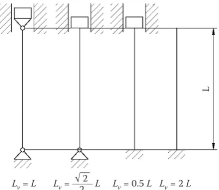
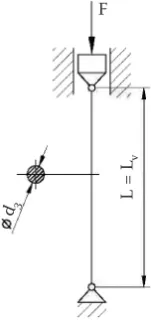
By the formulation of Euler’s Eq. (7) is it clear that the critical force – load is dependent on the slender-ness ratio (1). A slenderslender-ness ratio is then dependent on the buckling length of the bar and on the radius of gyration. The buckling length is dependent on the bar length and its way of fit (Figure 1). The four main kinds of the bar fit may be achieved by solving the differential equation of the deflection curve (Kuba 1977), loaded by an axial force. The combination of the previously described cases of fits and loads may be found in specific cases.
The calculation of the screw size is based on the classical theory of buckling. A screw is considered as a slender prismatic bar. The kind of buckling is set by the slenderness ratio, the buckling area is determined as the area of semi elastic buckling – Tetmayer’s area or elastic buckling area – Euler’s area (Höschl 1971).
The slenderness ratio is then described as the relation of the buckling length and the radius of momentum.
LV
λ = ––– (1)
i
Where square of radius of momentum is the ra-tio of minimal quadratic bending moment and the minimal area of the screw cross section (4).
I
min
i =
√
–––– (2)S3 π × d34
Imin = –––––– (3)
64 π × d32
S3 = –––––– (4)
4
If Eqs. (3) and (4) are put into formula (2), the calculation is obtained leading to the momentum radius determination.
d3
i = –––– (5)
4
If the formula above (5) is put into Eq. (1), the searched equation of the slenderness ratio of the motion screw is obtained. LV is the screw
buck-L
√ 2
Lv = L Lv = –––– L Lv = 0.5 L Lv = 2 L 2
[image:2.595.64.282.521.710.2]ling length dependent upon the form of bearing (Höschl 1971), and d3is the minimal diameter of the screw thread.
4 × LV
λ = –––––– (6)
d3
The process interdependence of the critical stress of the slenderness ratio in the area of elastic buckling (Figure 2) is established as the ratio of the critical force and the minimal area of the screw cross sec-tion (4).
π2 × E × I
min
F
KR LV2 π2 × E
σKRE = –––– = ––––––––– × –––––– (7) S3 S3 λ2
The process interdependence of the critical stress of the slenderness ratio in the area of semi-elastic buckling is established by Tetmayer`s formula, where a and b are tensions (9), (10), (Höschl 1971; Marghitu 2001; Zachariáš 2005).
σKRT = a – b × λ (8)
The relations leading to the tension dimension are deducted using the straight line relation.
Re – σU
a = Re + λk × ––––––––– (9)
λm – λk
Re – σU
b = ––––––––– (10)
λm – λk
The process of the critical stress interdependence with the slenderness ratio of classical pressure area is equal to the yield strength.
σKRD = Re (11)
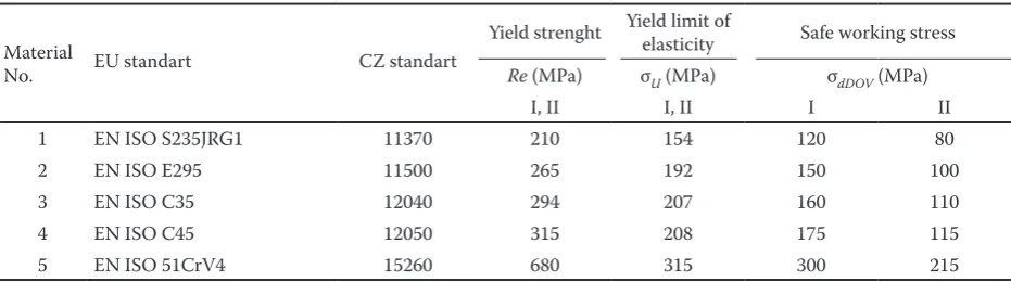
The relevance of relations (7), (8) a (11) is bound by the limit values of the slenderness ratio; these values are dependable on the motion screw mate-rial (Tables 1 and 2) (Höschl 1971; Orlov 1979; Bolek & Kochman 1990; Marghitu 2001; Zachariáš 2005), where condition I corresponds with the constant operational force load, and con-dition II means load by fluctuating operational force.
If the above given formulas are figured graphically, a classical graph of interdependence between the critical buckling stress and the slenderness ratio is obtained (Figure 2).
σKRD
σdE
σdT
σdD
σKRE
σKRT
classical pressure
area semi elastic area
elastic area λk
λ λm λu
Re
σU
σdDOV
[image:3.595.65.365.60.255.2]σcccccc σU
[image:3.595.65.531.626.756.2]Figure 2. Dependencies of critical stress and a limit safety stress upon the slenderness ratio
Table 1. Mechanical properties of motion screws materials
Material No.
Yield strenght Yield limit of elasticity Safe working stress
EU standart CZ standart
Re (MPa) σU (MPa) σdDOV (MPa)
I, II I, II I II
1 EN ISO S235JRG1 11370 210 154 120 80
2 EN ISO E295 11500 265 192 150 100
3 EN ISO C35 12040 294 207 160 110
4 EN ISO C45 12050 315 208 175 115
Regarding the screw stress when in motion; there is a raised risk of stability loss in comparison with that in the case of rod motionless bearing. The relation between the safety factor and the increasing value of the slenderness ratio exists in the case of the motion screw being selected with a consideration of the screw motion and screw stress by axial operational force.
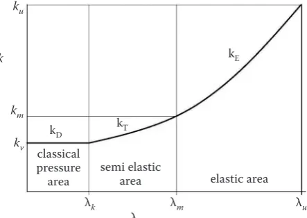
Through the calculations of the motion screws a higher safety margin is required of buckling ever more the higher is the value of the screw slenderness. Since the slenderness ratio is not known in advance, it is very difficult to quantify the safety margin (Fi-gure 3). To simplify the motion screw calculations, a method is used of stress decreasing along with increasing slenderness.
The safe working stress at slenderness λ is desig-nated as σd. The buckling safety margin is determined by the ratio of the critical stress to the safe working stress (Höschl 1971; Kuba 1977; Marghitu 2001; Zachariáš 2005).
σKR
kv = ––––– (12)
σd
In the area of classical pressure, it is possible to describe the value of the buckling safety margin
by the following equation as the ratio of the elastic strength to the safe working stress in the case of simple pressure.
Re
kv = kd = ––––– (13)
σdDOV
In the area of semi-elastic buckling, safe working stress is described using the following formula
σd = a× – b× × λ (14) where a× a b× are tensions (15), (16), (Höschl 1971; Marghitu 2001; Zachariáš 2005).
The relations leading to the tension dimension are deduced using the straight line relation (Figure 3).
σdDOV – σU a× = σ
dDOV + λk–––––––––– (15)
λm – λk
σdDOV – σU
b× = –––––––––– (16)
λm – λk
It is also possible to simply determine the buckling safety margin at marginal slenderness λm
σU
km = –––– (17)
σU
The adapted yield elastic limit σU is simply ob-tained from the equation given above in the area of semi-elastic buckling, it is possible to describe the value of the buckling safety factor according to the following formula; as the ratio of the critical stress in the area of semi-elastic buckling (8) divided by the safe working stress in the area of semi-elastic buckling (14).
a – b × λ
kV = kT = –––––––––– (18) a× – b× × λ
In the area of elastic buckling, the safe working stress is described by the following formula:
C
σd = –––– (19)
[image:4.595.64.534.72.201.2]λH
Table 2. Parameters buckling properties of motion screw materials
No.
Classical pressure
slenderness ratio slenderness ratioMarginal slenderness ratioMaximal Low buckling safety Marginal buckling safety Maximal buckling safety
λk λm λu kD km ku
I II I, II I, II I II I II I II
1 40 25 116 200 1.75 2.63 3.5 5.25 10 15
2 40 25 104 200 1.77 2.65 3.5 5.25 10 15
3 40 25 100 200 1.84 2.67 3.5 5.25 10 15
4 40 25 100 200 1.80 2.74 3.5 5.25 10 15
5 40 25 81 200 2.27 3.16 3.5 5.25 10 15
kD
classical pressure
area semi elastic area elastic area λk
λ λm λu
kT
kE ku
kmm
km
kv
[image:4.595.66.288.576.733.2]In the area of elastic buckling it is possible to describe the value of the buckling safety factor ac-cording to the following formula; as the ratio of the critical stress in the area of elastic buckling (7) di-vided by the safe working stress in the area of elastic buckling (19).
π2 × E
λ2 π2 × E
kV = kE = –––––– = ––––––– × λH–2 (20) C C
λH
The safe working stress in the area of semi-elas-tic buckling (19) can be obtained by the following equation, where β is the factor of tangential stress (Zachariáš 2005) dependant on the number of threads.
β × F
σd = a× – b× × λ = –––––– (21) S3
If Eqs. (6) and (4) are substituted into the previous formula, a relation is obtained describing the dimen-sion of the safe working stress in the area of semi-elastic buckling on minimal screw diameter d3.
4 × LV β × F
σd = a× – b× × –––––– = ––––––– (21) d3 π × d32
4
By the adaptation of formula (22), a quadratic equation in a normed form is obtained.
4 × β × F a× × d
32 – b× × 4 × LV × d3 – –––––––– = 0 (23) π
By solving this formula, the following equation of the minimal screw diameter calculation is obtained. However, the validity of this formula is limited to the semi-elastic buckling area.
4 ×β × F b× × 4 × LV ×
√
(b× × 4 × LV)2 + 4 × a× ×( π
)
d3 = –––––––––––––––––––––––––––––––––– (24) 2 × a×
The validity of the previous equation is limited by the straining force FDM, at marginal slender-ness of the screw. If Eqs. (6), (14) are substituted put into formula (21), the following relation is obtained.
β × FDM a× – b× × λ
m = –––––––––– (25)
π ×
(
4 × LV)
2λm
4
An equation describing the dimension of the ultimate force is obtained by the adaptation of the previous formula.
Lv 1 FDM = (a× – b× × λ
m) × π × 16 ×
(
–––)
2
× –– (26) λm β
The safe working stress in the area of elastic buckling (19) can be figured by the following equation, where β is the factor of tangential stress (Zachariáš 2005) and is dependant on the number of threads.
π2 × E
C λ2
σd = ––– = ––––– (27)
λH kE
If both marginal conditions (screw marginal slen-derness and maximal screw slenslen-derness) are put into the previous formula, an equation system of two unknown parameters is obtained.
C π2 × E
––– = ––––––– (28)
λmH k m× λm2
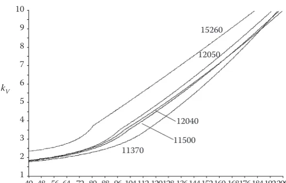
10 9 8 7 6 5 4 3 2 1
kV
40 48 56 64 72 80 88 96 104 112 120 128 136 144 152 160 168 176 184 192 200 λ
11370
15260
12050
12040
[image:5.595.63.358.549.738.2]11500
C π2 × E
––– = ––––––– (29)
λuH k u× λu2
If the system of equations is finally solved, then the value of H exponent is obtained and, by reverse substitution to the (28), (29) equation system, C coefficient value is obtained.
km × λm2
log ku × λu2
H = –––––––––––––– (30)
log λm
λu
If Eqs. (29) and (30) are substituted to Eq. (27), a formula describing the safe working stress in the elastic buckling area at minimal screw diameter d3 is achieved.
C β × F
σd = –––––––– = –––––––– (31)
(
4 × LV)
H π × d32d3 4
By the arrangement of the previous equation a for-mula is obtained describing the size of the minimal screw cross section. The validity of this equation is limited by the area of elastic buckling.
4 × β × F 1
d3 =
(
–––––––– × (4 ×LV)H)
H+2 (32)π × C
The equations described previously may be pre-sented graphically (Figure 4) by the substitution of the material coefficients obtained (29), (30) and (Tables 1 and 2) to the equations of buckling safety. In view of clarity, only dependencies are pictured regarding the constant straining force. Similar de-pendencies are then achieved, where the fluctuating straining forces material parameters are substituted to the equations mentioned.
The formulas describing the design of the motion screw parameters regarding the screw drift during the operational strain are derived in a previous part of the article. The tangential stress also arises in the motion screw. This is caused by the screw torsion by a couple of frictional forces during the relative movement of the screw and the nut. If the screw stress is considered also from the point of torsion and the press stress at same time, it is worthy to check the screw under the classical strengths con-ditions.
Both of the strains are then converted into the reduced screw pressure. The motion screw reduced stress is set by Mohr’s hypothesis.
σd = σred = √ σ2 + 4 × τ2 (33) The direct stress formed during the screw strain is expressed by the following formula.
4 × F
σ = –––––– (34)
π × d32
The tangential stress caused by the screw torsion strain may be expressed as the ratio of the moment necessary to break the thread friction and the screw torsion section modulus.
M
z
τ = –––– (35)
Wk
The moment necessary to break the thread fric-tion is extracted by following formula (Zachariáš 2005), where: α is an angle of the thread pitch, φ is the friction angle of the screw thread, d2 is the pitch diameter of the screw thread.
Mz =0.5 × F × d2 × tan(α + φ) (36) The torsion section modulus is described by the following equation.
π × d33
Wk = –––––– (37)
16
The relation between the pitch diameter of the screw thread and the minimal diameter of the screw thread is figured in the following formula, where d is the diameter of the screw shank. The formula is accurate enough in the case of the strength calcula-tion even though there are other, more precise and complicated equations describing the screw shank and other parameters and dependencies.
d + d 3
d2 = –––––– (38)
2
If formulas (36), (37), (38) are installed into for-mula (35), the following equation is obtained.
L
=
Lv
F
[image:6.595.132.208.65.227.2]d3
4 × F d
τ = ––––– × (1 + ––––) × tan(α + φ) (39) π × d32 d3
By implementing formulas (34) and (39) to Eq. (33) the sought formula is obtained describing the dimension of the reduced direct stress. This stress has to be equal to the safe working stress (21). 4 F d
σd = σred = ––––– ×
√
1 + 4 ×[(
1 + ––)
× tan(α + φ)]
2 = π × d32 d34 × F
= β × ––––––– (40)
π × d32
By the modification of the previous equation and the expression of the tangential stress β, the formula is obtained of the real factor of the tangential stress influence.
d
βS =
√
1 + 4 ×[(
1 + ––)
× tan(α + φ)]
2 (41) d3During the screw control, the real factor of the tangential stress influence has always to be smaller than or equal to the factor of tangential stress influ-ence βs ≤ β.
RESULTS
Calculation parameters of 11500 steel (EN ISO E295)
The designing parameters sought are obtained when 11500 (EN ISO E295) material constants (Ta-bles 1 and 2) are implemented to the formulas (26), (24), (32), (18), (20).
L
V 1
FDM =
(
–––––)
2 × ––– (42) 3.961 β(β × F)0.1783 × L
V0 .6434
d3 = ––––––––––––––––– (43)
15.9114 L
V LV β × F
d3 = –––– +
√(
––––)
2+ ––––––– (44) 70.5 70.5 164.54λ S3
kVTS =
(
310.6 – ––––––)
× –––– (45) 0.877 β × Fπ2 × E × S 3
kVES = ––––––––––– (46)
λ × β × F
Calculation process
Design sizes of the motion screw of the manual jack (Figure 5). The screw is made of 11500 (EN ISO
E295) steel and the bolt is made of cast iron, fric-tional angle is φ = 6°. The acting force F = 22 000 N, the buckling length LV = 560 mm.
By Eq. (42), the size of the limit force, is set where β = 1.3 is the factor of the tangential stress influences of simple start thread.
1 LV 1 560
FDM = ––– ×
(
–––––)
2 = ––– ×(
–––––)
2 = 15 375 N (47) β 3.961 1.3 3.961The kind of buckling is determined by comparison of the operational and the limiting forces
Fprov = 22 000 N > FDM = 15 375 N
Because Fprov > FDM , the following calculations are done in the area of inelastic (rigid) buckling.
By formula (44) the diameter of the screw core is determined.
l
V LV β × F 560
d3 = –––– +
√
(
–––––)
2 + –––––– = ––––– + 70.5 70.5 164.54 70.5 560 1.3 × 22 000+
√
(
–––––)
2+ ––––––––––– = 23.33 mm (48) 70.5 164.54By means of the table of regular trapezes threads, the following parameters are selected (Zachariáš 2005):
Tr 32 × 6, d = 32 mm, d3 = 25 mm, D1 = 26 mm, P = 6 mm, S3 = 491 mm2, d
2 = 29 mm, . P 6
α = arctan × –––––– =arctan × –––––– = 3.8° π × d2 π × 29
The screw slenderness is determined by formula (6) 4 × LV 4 × 560
λ = –––––– = ––––––– = 89.6 (49) d3 25
It is now possible to check the screw safety margin in the case of buckling by formula (45)
(310.6 – λ/0.877) × S3 (310.6 – 89.6/0.877) × 491 kV = –––––––––––––––– = –––––––––––––––––– = β × F 1.3 × 22 000
= 3.57 (50)
If the obtained value of the safety margin (50) is compared with the limiting safety margin, it is pos-sible to read out from the safety graph (Figure 4.) and figure out that the screw corresponds to the conditions of safety buckling, meaning it will not turn aside.
As a last but not least step, the screw is controlled by strength, according to Eq. (41) the real factor is determined of tangential stress influence.
screw is in concordance with the strength conditions (Zachariáš 2005).
d
βS =
√
1 + 4 ×[(
1 + –––)
× tan (α + φ)]
2 = d332
=
√
1 + 4 ×[(
1 + –––)
× tan (3.8° + 6°)]
2 = 1.27 < β = 1.3 (51) 25DISCUSSION
The assessment of the motion screw has been, frequently discussed for decades. There are tens of ways of calculation, design and stability control of the motion screw. However, up to now, no simple instruction exists determining which method is the most suitable. The decision is on the constructors shoulders. The constructor or the designer has to make the decision based on his own skill, knowledge, the complete analysis of the system and environ-ment where the designed mechanism is going to be applied.
When the standard and well known case of the motion screw mechanical stress is to be solved, the solution being approved by long term experiments and practical experience, it is very useful to use analytical – empiric methods. Some of these meth-ods are the so called iterative methmeth-ods and others provide immediate results. The method described above is to calculate and design standard sizes of the motion screws parameters and their stability control. Maximum load capacity (pressure) method is a kind of non – iterative methods representing an analytical method which utilises empiric safety coef-ficients. Such method is evolved to facilitate most effectively the motion screw design, its stability and strength. The method is based on long term practi-cal experience gained during the last 50 years of the motion screws designing for many kinds of human working applications.
At the present time, the mostly used classi-cal analyticlassi-cal-empiric methods are derived from the two basic theories of buckling – Tetmayer’s semi-elastic buckling, and Euler’s elastic buckling theories. By the combinations of purely theoretical methods and empiric knowledge obtained dur-ing the past 150 years tens of methods, have been derived which are, currently in use. Each of these specific methods is recommended for a certain case of design and solution of a defined problem (steel bridges constructions, building sites support pil-lars, beams, armatures, aviation industry, railway system design etc.). Such methods are also used for designing many different materials usage (plastic,
steels, metals, woods, cold short materials as well as ductile materials).
Among the most widespread methods used in calculations on the worldwide scale are: Rankin and Gordon Formula (applied for designing the bridge constructions), Straight Line Formula (for carrying columns of buildings, columns of bridges), Formulas of the American Railway Engineering Association (railway bridges, beams, railway constructions), Johnson’s Formula (steel bars, beams), Formulas of the American Institute of Steel Construction (steel bars and braces), Formulas of pipe columns ( hol-low bars, holhol-low carrying columns) and others such as: (Faires 1955; Oberk et al. 2000; Marghitu 2001).
Many different numerical methods may be used to solve the motion screw stability. Such proce-dures are frequently used in the cases where the limiting conditions are changed upright or during the operation, in the dependency on time. The limiting conditions are changed linearly or non-lin-early: (medicine, osseous or joint implants, highly strained constructions placed on a soft basis like soils, plastic matters, and so on). An other case is if the stressing forces change with time, as well as their size and direction or if the environment where the mechanism works is completely changed – the heat transfer has to be taken into account (extrud-ers, blast furnace mills, food lines, glasshouses etc.). Another specific case is if the mechanical unit contains tens of motion screws strained by different stresses, however, the stressing forces are depend-ent on the force coming into the system (cyber – robotic systems, industrial robots, space shuttles, motion control systems etc.), or if to final tension of the motion screws is in the area of elastic deforma-tion – combinadeforma-tions are then mostly used of FEM and FVM or other numerical methods (forming process of screw spike, special elements forming, pre-strained constructions, utilisation of the limit phases etc.) (Maurer et al. 2001; Weronski et al. 2005; Fabre et al. 2005).
The mechanical structure of the machine and the drive features may be described in most of cases using the so called Flexible Multi-Body System. The methodology of creating the system of several plastic bodies is commonly used when solving the stability and the drive by the ball screw. Each plastic body is modeled using FEM, while all of the plastic bonds between the bodies are substituted by combined bodies of spring-absorber. By the kinematical bonds, it is possible to assembly a model of the ball screw drive. The model of the ball screw drive is usually webbed by FEM elements, other parts of the drive are modelled using solid bodies and plastic bonds among them.
While solving the buckling stability of slender bars in the Euler’s area of elastic buckling, Newton – Raphson method may be used utilising computer programs such as FEM, which is able to proceed the equation systems of geometrically non linear problems. The computing procedure utilises an al-gorithm of gradual directives for different numbers of webbed elements. In the case of ANSYS program, such procedure is defined as linear buckling and the model is webbed by the classical element BEAM3. Critical buckling force calculation is affected by a number of the elements divisions.
CONCLUSION
A current random observer would not be able to count the numbers of the surrounding motion screws. These are literally everywhere, even though they are not often visible. Motion screws are inte-grated in the constructions which influence every single day of human beings. What is common for: bread, beer, hospital bed, roller coasters, football stadiums, theaters, airplanes, paper, steel, glass, pure water, plastic, trains, cars, satellites, measuring devices, coins, and millions of other things? Motion screws, either straightly integrated in the construc-tions or just participating in the production of the items mentioned.
There are tens of ways of the motion screws design at present. These are methods using pure theoretical foundations as well as methods purely empirically based. Currently are used aggrandised calculations with the computer support such as FEM.
The calculation method of the motion screw design described above and using the stress limit values is a combination of the limit situation and the empiric values obtained by long-term practical usage of the motion screws. This theory is combined with the classical buckling theory and uses empirical
val-ues obtained by a long time research which started already at the time of the first bi-plane designing about hundred years ago.
The steps of the calculation described above are not iterative, such kind of design being more than suitable for students and inexperienced young construction workers and designers. On the other hand, it is obvious that the described method can not substitute the knowledge of a designer obtained by many years of experience in constructing and the design practice.
A control graph of the buckling safety coefficients to prevent the screw buckling out is also derived in the article. The described dependencies are de-duced for the motion screws loaded with a static force. The safety dependency for screws loaded by fluctuating forces may be easily obtained using the calculation described above, and by the correct substitution of the material constants and the limit safety values.
The complete design of the motion screw made out of 11500 (ISO EN E295) steel and loaded with a static force is fully described in the article. The exact calculation equations are obtained if the theoretical equations mentioned above, as well as specific material and buckling safety constants are correctly used.
References
Bolek A., Kochman J. (1989): Části strojů. Svazek 1, SNTL, Praha.
Bolek A., Kochman J. (1990): Části strojů. Svazek 2, SNTL, Praha.
Fabre A., Lillamand I., Masse E., Barrallier L. (2005): Neutron evaluation of stress in industrial screws. Materials Science Forum, Vol. 490, Trans Tech Publication, Schwit-zerland, 269–274.
Faires V.M. (1955): Design of Machine Elements. The Mac-millan Company, New York.
Höschl C. (1971): Pružnost a pevnost ve strojnictví. SNTL, Praha.
Kuba F. (1977): Teorie pružnosti a vybrané aplikace. SNTL, ALFA, Praha.
Marghitu D.B. (2001): Mechanical Engineers Handbook. Auburn University Alabama, Academic Press, Auburn. Maurer P., Schubert J., Holweg S. (2001): Finite element
analysis of a tandem screw configuration in sagittal split osteotomy using biodegradable osteosynthesis screws, International Journal of Adult Orthodontics and Ortho-gnathic Surgery, 16: 300–304.
Oberk E., Jone F.D., Horton H.L., Ryffel H.H. (2000): Machinery’s Handbook. 26th Ed., Industrial Press Inc.,
Orlov P.I. (1979): Základy konštruovania. VTEL, Bratis-lava.
Weronski W., Gontarz A., Pater Z. (2005): Forming process of screw spike in double configuration. In: VIII Int. Conf. Computational Plasticity – COMPLAS VIII, CIMNE, Barcelona.
Abstrakt
Herák D., Karanský J., Chotěborský R. (2008): Využití teorie mezního dovoleného tlakového napětí při návrhu rozměrů pohybových šroubů. Res. Agr. Eng., 54: 32–41.
Článek popisuje postup návrhu pohybového šroubu dle metody mezního tlakového napětí. V článku jsou odvozeny výsledné obecné vztahy pro návrh pohybového šroubu a také vyčísleny rovnice pro výpočet pohybového šroubu vyrobeného z oceli 11500 zatěžovaného statickou provozní silou. Nedílnou součástí článku je odvození rovnic bez-pečnosti proti vybočení šroubu a jejich grafické zobrazení.
Klíčová slova: Euler; Tetmayer; pohybový šroub; štíhlostní poměr; napětí; vybočení šroubu
Zachariáš L. (2005): Části strojů. ČZU, Praha.
Received for publication July 8, 2007 Accepted after corrections August 6, 2007
Corresponding author:
Ing. David Herák, Ph.D., Česká zemědělská univerzita v Praze, Technická fakulta, katedra mechaniky a strojnictví, Kamýcká 129, 165 21 Praha 6-Suchdol, Česká republika