Numerical Analysis of Solidification Effect on Diffusion Measurement in Liquid using the Long Capillary Method

Numerical Analysis of Solidification Effect on Diffusion Measurement in

Liquid using the Long Capillary Method

Kenichi Ohsasa

, Atsushi Hirata

, Misako Uchida

_{and Toshio Itami}

1

Division of Molecular Chemistry, Graduate School of Engineering, Hokkaido University Sapporo 060-8628, Japan

2_{Technical Development & Engineering Center, Ishikawajima-Harima Heavy Industries Co., Ltd., Yokohama 235-8501, Japan} 3_{Space Utilization Research Center, National Space Development Agency of Japan, Tsukuba 305-8505 Japan}

A numerical analysis was carried out to examine the solidification effect on the concentration distribution of a solute in an Ag/Ag–5 at%Au diffusion couple in a liquid diffusion experiment using the long capillary method. Shrinkage-induced fluid flow in the solidifying sample was calculated, and the solute movement due to the fluid flow was evaluated. In the analysis, molten samples in a graphite crucible were cooled in air at three different cooling rates. Flat isoconcentration contours in the horizontal plane of the diffusion couple were formed in the sample with a low cooling rate, whereas concave isoconcentration contours were formed in the samples with high cooling rates. Those features in the simulation agreed with the experimental results. The optimum conditions to avoid the solidification effect in liquid diffusion experiments are discussed.

(Received December 9, 2002; Accepted April 4, 2003)

Keywords: diffusion, solidification, silver-gold, long capillary method

1. Introduction

The long capillary method is a simple method to measure the diffusivity of an element in liquid.1)Molten alloys with different compositions are joined in a long cylindrical crucible with a small diameter, and the natural convection in the sample can be restricted due to its configuration. The diffusion coefficient of an element can be determined from the concentration profile measured after the completion of the solidification of the sample. Advantages of the capillary method are its simple configuration and high cost perfor-mance. However, even if buoyancy-induced fluid flow such as thermal or solutal convection in the sample is restricted, the concentration profile of an element in liquid may be changed during the solidification by the solidification shrinkage-induced fluid flow. In spite of the importance of the solidification effect on diffusion experiments, much attention has been paid to the restriction of convection in the sample, and little attention has been given to the solidification effect in experiments using the long capillary method. To measure correct diffusivity of elements in liquid, it is highly desirable to estimate the solidification effect on the experi-ment using a liquid diffusion couple.

The aims of this study are: 1) to establish a basic mathematical model for the solidification process in diffusion experiments using the long capillary method and 2) to analyze the solidification processes of samples to find the most desirable cooling conditions to carry out long capillary experiments. To confirm the applicability of the model, simulated results were compared with experimental results.

2. Method

2.1 Conditions of diffusion experiment

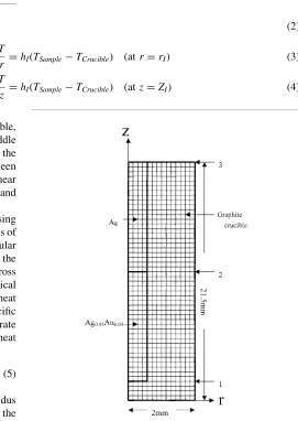
An Ag/Ag–5 at%Au diffusion couple was melted using an electric furnace in a graphite crucible with a cylindrical shape

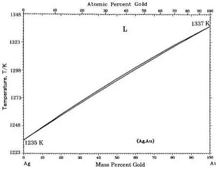
of 1 mm in inside diameter, 21.5 mm in height, 2 mm in wall thickness and 1.5 mm in bottom thickness. The lengths of Ag and Ag–5 at%Au specimens were both 10 mm and they were joined in the crucible. The Ag–Au binary system is completely miscible in both solid and liquid regions as shown in Fig.12)and it is seen that solidification range of the Ag–Au alloy is very narrow. Unevenness of solute distribu-tion in an alloy after solidificadistribu-tion is known as macrose-gregation and it is expected from the features of the Ag–Au diagram that severe macrosegregation will not occur. This is the reason why the Ag–Au alloy system was chosen as the specimen for the liquid diffusion experiment. The Ag specimen is located on the Ag–5 at%Au alloy specimen in the graphite crucible and hence the solutal convection can be restricted because the density of the Ag–5 at%Au alloy is higher than that of Ag. The molten sample was kept at 1250 K for a certain period and then the furnace was moved upward and the crucible was exposed to air. The sample was allowed to cool and the upper part of the sample was hotter than the lower part due to the radiation effect of the furnace located

Fig. 1 Ag–Au binary phase diagram.

*_{Present address: Material Department, Research Laboratory,}

just above of the sample. The cooling rate of the sample could be controlled by the height of the furnace. Because a temperature gradient exists in the sample,i.e., the density at the upper part of the sample is low, the thermal convection in the sample can be restricted. After the completion of the solidification, the sample was cut into vertical cross sections, and Au concentration distributions in the sections were measured using an EPMA. The detail results of the experi-ment were reported in another paper.3)

2.2 Numerical model

The conduction of heat in both the specimens and crucible

was calculated by solving the basic heat conduction equation in the form of axial symmetry.

@T @t þ

1

rUrTþUr @T

@r þUZ @T @Z ¼

@2T @r2 þ

1

r @T

@r þ @2T

@z2

ð1Þ

The mathematical expressions for the boundary conditions at the center of the sample and the sample-crucible interface were as follows.

@T

@r ¼0 ðatr¼0Þ ð2Þ

Sample @T

@r ¼ Crucible @T

@r ¼hIðTSampleTCrucibleÞ ðatr¼rIÞ ð3Þ

Sample @T

@z ¼ Crucible @T

@z ¼hIðTSampleTCrucibleÞ ðatz¼ZIÞ ð4Þ

As the boundary condition at the outer surface of the crucible, measured temperatures at three positions of upper, middle and lower of the crucible surface were used. In the calculation, temperatures at the crucible surface between the measured positions were estimated by making linear interpolation. An adiabatic condition was used at the top and bottom surfaces of the sample.

In order to solve eqs. (1) through (4) numerically by using the finite difference method, the longitudinal cross sections of the specimens and crucible were divided into rectangular grids with 0.1 mm on the r- and z-coordinates. Since the shape of the sample was axial-symmetric, half of the cross section was divided as shown in Fig.2. In the numerical calculation of the heat conduction involving the latent heat evolution during the solidification of the sample, the specific heat in the solidification range was increased to incorporate latent heat evolution based on the equivalent specific heat method.3–6)

C_P0 ¼CPþH

T ð5Þ

T in eq. (5) is the solidification range between the liquidus and solidus temperatures, which varies depending on the concentration of Au in the grid. Since Ag is a pure element and does not have a solidification range, an apparent solidification range of 0.5 K was assumed for use eq. (5), and the Ag–Au phase diagram was modified as shown in Fig.3. The liquidus and solidus temperatures, solidification range and solid fraction of a grid having a concentration ofC0

were expressed as follows.

TL¼T0þmLC0 ð6Þ

TS¼T0þmSC00:5 ð7Þ

T ¼ ðmLmSÞC0þ0:5 ð8Þ

fS¼TLT

T ðTS<T<TLÞ ð9Þ

In the long capillary experiment, buoyancy-induced

con-vection can be restricted by its configuration; however, solidification shrinkage-induced flow is unavoidable. Until now, many models predicting macrosegregation of alloys have been proposed.7–17) These models involve buoyancy-induced and shrinkage-buoyancy-induced flows. In the present study, fluid flow is induced only by solidification shrinkage, and accurate prediction of shrinkage-induced fluid flow is required. We adopted the method proposed by Ohnaka et al.18–20)to calculate the shrinkage-induced fluid flow during the solidification of the diffusion couple.

The finite difference form of the mass conservation equation in a grid with consideration of solidification shrinkage is expressed as follows.

X

n

Lf_LnSnUnt¼ ðSLÞVi;jfSi;j ð10Þ

The left-hand side of eq. (10) expresses the amount of mass flow into or out from the grid ði;jÞand the right-hand side expresses the solidification shrinkage in the grid ði;jÞ. The change of the solid fraction,f_Si;j, was calculated from the heat transfer analysis described above. Above the grids at the top of the sample, virtual grids with 1atmpressure are placed and liquid Ag can always be supplied from the grids to compensate for the solidification shrinkage of the sample.

The velocity of flow in a solidifying alloy is calculated by Darcy’s law describing the fluid flow in a porous medium

Un¼ K

fn L

PnPi;j

d

ð11Þ

where d¼z for z direction and d ¼r for radial direction. Since the permeabilityKin a pure Ag and Ag–Au alloy system could not be found in the literature, the permeability evaluated in a Al–Cu alloy20)was used in the present study.

K¼6:01011f_L2:0 ðfL<fLCÞ

K¼2:24107f_L80:0 ðfLC<fLÞ where fLC¼0:9

ð12Þ

The limiting solid fraction for flow was assumed to be 0.7, and hence the permeability of the grid having a solid fraction higher than 0.7 becomes 0 and liquid does not flow through the grid. To examine the effect of permeability on the flow calculation, the permeability calculated from the Kozeny-Carman equation12,21)was also used; however, the difference between the two calculated results was small, and only the results using the permeability in eq. (12) was described in this paper.

The solute conservation in grid ði;jÞ is expressed as follows.

Vi;jCi;j¼L

X

n

SnUnCut _ð13Þ

In eq. (13), ¼SfSþLfL, Ci;j is the change of the

concentration in the grid ði;jÞ at the time interval t (1:6105_{s). The upstream interpolation method was used}

for Cu, i.e. Cu¼Ci;j when Un <0 and Cu¼Cn when Un>0.

In eq. (13), mass transfer due to chemical diffusion is neglected because the mass transfer due to diffusion is very small in comparison with that caused by fluid flow.

2.3 Initial conditions and calculation procedure Experimentally measured temperatures at the crucible surface just before the start of cooling of the sample are given for both the specimens and crucible. The initial concentration distribution along with the z axis of the sample was calculated from eq. (14) with the assumption that the diffusion coefficient,D, of Au in liquid is1:0108(m2/s)

Cðz;tÞ ¼C0 1:0erf z

2pffiffiffiffiffiDt

ð14Þ

where erf is the error function and the concentration distribution in the radial direction is assumed to be uniform. Initial pressure of each grid is 1atmpressure.

The calculation procedure is as follows. The new tem-perature in each grid after each time steptwas calculated from eqs. (1) through (4) and the change in the fraction solid fsi;j in each grid was calculated from eq. (9). The new pressure of each grid,Pi;j, was calculated by eliminatingUn from eqs. (10) and (11). The new velocity of flowUnbetween each grid was calculated from eq. (11) and the new solute concentration of each grid,Ci;j, was calculated from eq. (13). The calculation procedure was repeated until the completion of the solidification. If the grids having a solid fraction higher than 0.7 aligned in the radial direction from the center to the surface of the specimen, the flow channel was blocked, and the calculation was interrupted. The properties used in the calculation are shown in Table 1.

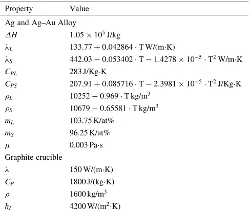
Table 1 Properties used in the calculation.

Property Value Ag and Ag–Au Alloy

H 1:05105_J/kg

L 133:77þ0:042864TW/(mK)

S 442:030:053402T1:4278105T2W/mK CPL 283 J/KgK

CPS 207:91þ0:085716T2:3981105_T2_J/KgK L 102520:969Tkg/m3

S 106790:65581Tkg/m3 mL 103.75 K/at%

mS 96.25 K/at%

0.003 Pas

Graphite crucible

150 W/(mK)

CP 1800 J/(kgK)

1600 kg/m3

hI 4200 W/(m2_K)

3. Results and Discussion

3.1 Changes in temperature field in the sample

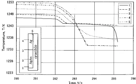
Solidification processes of diffusion couples with three different cooling rates were simulated using the numerical model described above. Figure4 shows measured cooling curves at the surface of the crucible with the average cooling rate of 0.3 K/s. Those cooling curves were used as the initial and boundary conditions of the calculation of heat conduc-tion at the crucible surface. The time axis of Fig.4is scaled from 470 s because the real time lapse in the experiment is used and it is seen that a temperature gradient in the z-axis exists at the crucible surface due to the influence of the furnace. Figure5 shows calculated cooling curves at the center of the diffusion couple sample, and it is seen that the lower Ag–Au region solidifies at 1244 K, while the upper Ag region solidifies at the melting point of Ag of 1235 K. The upper Ag region is maintained at a higher temperature during most of the experimental period except for a short period at about 500 s. Changes in the fraction solid distribution along the z-axis of the sample are shown in Fig. 6and solidification proceeds unidirectionally from the bottom to the top of the sample.

Figure7shows calculated cooling curves in the diffusion couple sample with an average cooling rate of 22.1 K/s. In the early stage of the experiment, the temperature of the upper Ag region is higher than that of the lower Ag–Au region, and then the temperatures of the upper Ag and joined regions fall

below the temperature of the lower Ag–Au alloy region because the lower alloy region has a higher liquidus temperature than the melting point of pure Ag. Changes in the fraction solid distribution along the z-axis of the diffusion couple are shown in Fig.8and it is seen that the solidification does not proceed unidirectionally; furthermore, the calcula-tion was interrupted when a blockade occurred at the region near the joined interface.

3.2 Fluid flow and changes in the concentration profiles Figure9 shows shrinkage-induced fluid flow in the samples with the average cooling rate of 0.3 K/s and

Fig. 4 Measured cooling curves at the graphite crucible surface with average cooling rate of 0.3 K/s.

Fig. 5 Calculated cooling curves of the sample with a cooling rate of 0.3 K/s.

Fig. 6 Changes in the fraction solid distribution of the sample with a cooling rate of 0.3 K/s.

Fig. 7 Calculated cooling curves of the sample with a cooling rate of 22.1 K/s.

22.1 K/s. In the sample with the cooling rate of 0.3 K/s, the liquid flows from the top to bottom vertically to compensate for the solidification shrinkage of the lower region, whereas in the sample with the cooling rate of 22.1 K/s, bypass flow occurs around the solidified region or the region having high fraction solid of over 0.7 in which liquid does not flow.

Figure10shows Au concentration distributions along the z-axis of the solidified sample cooled with the average cooling rate of 0.3 K/s. The initial concentration distribution

of Au in liquid is also plotted in Fig. 10. The concentration is uniform for the radial direction and the concentration curves at the surface, 1=2Rand center overlap each other, but it is seen that the shape of the concentration curves moves downward from the location of the initial Au concentration curve due to the shrinkage-induced flow. Figure11shows Au concentration distributions along the z-axis of a solidified sample cooled with the average cooling rate of 22.1 K/s. A comparatively steep concentration gradient exists along both the radial and z-axial directions of the sample.

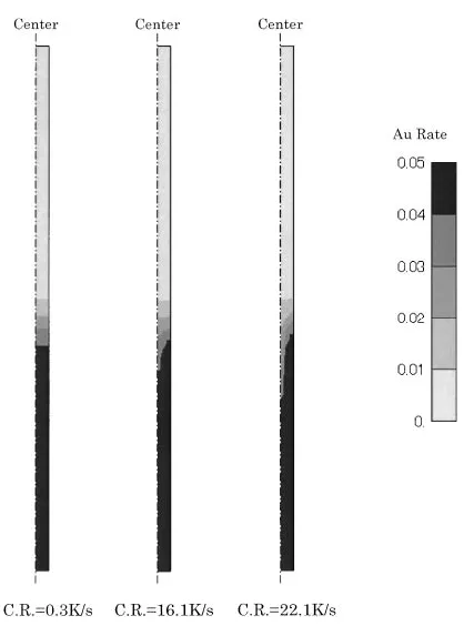
Figure12 shows isoconcentration contours in three sam-ples with different cooling rates. The sample with a low cooling rate exhibits flat isoconcentration contours with respect to the radial direction, whereas the samples with higher cooling rates exhibit concave isoconcentration

con-Fig. 9 Calculated fluid flow induced by solidification shrinkage in the samples with cooling rates of 0.3 K/s and 22.1 K/s.

Fig. 10 The final concentration distributions of Au along with the z-axis of the solidified sample with a cooling rate of 0.3 K/s.

0 0.01 0.02 0.03 0.04 0.05 0.06

0 2 4 6 8 10 12 14 16 18 20 Distance from Bottom, d/ mm

Au Rate

Center 1/4R 1/2R Surface Initial at Center

Initial at Center

Fig. 11 The final concentration distributions of Au along with the z-axis of the solidified sample with a cooling rate of 22.1 K/s.

tours, and it is seen that the depth of valley of the concave isoconcentration contour becomes deeper with increasing cooling rates. Those features of the calculated results were also observed in the experimental results.3)

3.3 Desired conditions for diffusion experiments The present numerical analysis has shown that the solidification shrinkage changes the concentration distribu-tion of the element in liquid and exhibited the considerable effect of solidification on a diffusion experiment using the long capillary method. The concentration distributions at the surface and center in the sample with a low cooling rate moved concurrently to the bottom as shown in Fig.10. In the samples with high cooling rates, the solute at the center moves deeper than that at the surface as shown in Fig. 11, and it seems that the concentration distribution at the surface is most similar to the concentration distribution that existed in liquid state. Based on the Boltzmann-Matano analysis, the inter-diffusion coefficient of an element in liquid is deter-mined from the concentration distribution in the sample,

Dðc0Þ ¼ 1 2t

dx dc

Zc0

0

xdc ð15Þ

wheretis diffusion time,dx=dcis inverse of the concentra-tion gradient at the concentraconcentra-tion, c0_{,. If the concentration}

distribution at the surface shown in Fig.11 is used to calculate the inter-diffusion coefficient, the error will increase at low concentration region. On the other hand, it seems that the error will be small if the concentration distribution in Fig.10is used because the integral term in eq. (15) is calculated with the coordinate in which the Matano interface is used as the original and the effect of the parallel movement of concentration distribution become small.

4. Conclusions

Solidification effects in a liquid diffusion experiment using the long capillary method have been examined by simulating the solidification process of an Ag/Ag–0.5 at%Au diffusion couple using a numerical model. Solidification shrinkage-induced flow was computed based on the heat transfer, Darcy’s flow and mass balance calculations. Solute move-ment due to the fluid flow was analyzed for three different cooling conditions. The Au concentration distribution in the sample with a low cooling rate was moved downward due to shrinkage-induced flow and a flat isoconcentration contour was formed. On the other hand, a concave isoconcentration contour was formed at the joined region in the samples with a high cooling rate. The obtained features from the numerical simulation were same with the experimental results and showed the applicability of the numerical model developed in the present study. The present study also showed the necessity of the some correction of the measured concentra-tion distribuconcentra-tion in liquid diffusion experiments using the long capillary method.

Nomenclature

C: concentration (at%) C0: initial concentration (at%) CP: specific heat (J/(kg K)) C0

P: apparent specific heat (J/(kg K)) C: concentration change in a grid D: diffusion coefficient (m2_/s) fL: fraction liquid

fS: fraction solid

fS: Change of fraction solid

hI: heat transfer coefficient at sample-crucible interface (W/(m2K))

H: latent heat (J/kg) K: permeability (m2) mL: liquidus slope (K/at%) mS: solidus slope (K/at%) P: pressure (Pa)

r: radial coordinate

rI: radius of cylindrical sample (m) r: grid size in r-direction (m) Sn: interface area between grids (m2₎ t: time (s)

t: time step (s) T: temperature (K)

T0: melting point of Ag (K) TL: liquidus temperature (K) TS: solidus temperature (K)

TCrucible: temperature of crucible (K) TSample: temperature sample (K) T: solidification range (K)

Ur: r component of flow velocity (m/s) Uz: z component of flow velocity (m/s) V: volume of a grid (m3₎

z: axial coordinate

ZI: position of the bottom of crucible (m) z: grid size in z-direction (m)

Greek Symbols

: thermal diffusivity (¼=CP)

: thermal conductivity of crucible (W/(m K)) : viscosity (pas)

: density (m3)

Subscripts and Superscripts

i;j: grid number L: solid

n: number of neighboring grids surrounding gridði;jÞ

S: liquid

REFERENCES

1) M. Shimoji and T. Itami:Atomic transport in liquid metals, (Trans Tech Publications, 1986) pp. 159–160.

2) T. B. Masalski:Binary Ally Phase Diagram, (ASM International, 1990) pp. 13.

4) D. J. P. Adenis, K. H. Coats and D. V. Ragone: J. Inst. Metals (1962– 1963) 395–403.

5) E. A. Mizikar: Trans. AIME239(1967) 1747–1753.

6) I. Ohnaka:Introduction of Computer Analysis for Heat Transfer and Solidification, (Maruzen, Tokyo, 1985) pp. 200–201.

7) M. C. Flemings and G. E. Nereo: Trans. AIME239(1967) 1449–1461. 8) M. C. Flemings, R. Mehrabian and G. E. Nereo: Trans. AIME242

(1968) 41–49.

9) M. C. Flemings and G. E. Nereo: Trans. AIME242(1968) 50–55. 10) W. D. Bennon and F. P. Incropera: Int. J. Heat Mass Transfer30(1987)

2161–2170.

11) W. D. Bennon and F. P. Incropera: Int. J. Heat Mass Transfer30(1987) 2171–2187.

12) C. Beckermann and R. Viskanta: Physico Chemical Hydrodynamics10

(1988) 195–213.

13) J. Ni and C. Beckermann: Metall. Trans.22B(1991) 349–361. 14) M. C. Schneider and C. Beckermann: Metall. Mater. Trans.26A(1995)

2373–2388.

15) C. Y. Wang and C. Beckermann: Metall. Mater. Trans.27A(1966) 2754–2764.

16) C. Y. Wang and C. Beckermann: Metall. Mater. Trans.27A(1966) 2765–2783.

17) C. Beckermann and C. Y. Wang: Metall. Mater. Trans.27A(1996) 2784–2795.

18) I. Ohnaka, T. Fukusako and K. Nishikawa: Tetsu-to-Hagane´67(1981) 547–556.

19) I. Ohnaka and K. Kobayashi: Trans. ISIJ26(1986) 781–789. 20) I. Ohnaka and M. Matsumoto: Tetsu-to-Hagane´73(1987) 1698–1705. 21) M. C. Schneider, J. P. Gu, C. Beckermann, W. J. Boettinger and U. R.