Use of Landsat images for yield evaluation within a small plot

It is generally known that topography plays an important role in the control of plant growth and that water is the most frequent limiting factor in agriculture (Schmidt and Persson 2003). Yield vari-ability is caused by many factors such as the plant and soil factors, weather (temperature and precipi-tation distribution) and topography. Consequently, the yield maps tend to vary from year to year.

The following topography attributes are used most widely for explaining topography influence on yield: digital elevation models (DEM) (Iqbal et al. 2005, Murphy et al. 2009), relative field elevation (Serrano et al. 2013), slope (Pilesjö et al. 2005), curvature (Guo et al. 2012), flow accumulation

(Marques da Silva and Silva 2008, Kumhálová et al. 2013), topography wetness index (TWI) (Schmidt and Persson 2003, Sørensen et al. 2006), distance to flow lines (Marques da Silva and Silva 2006) and compound topographic index(Momm et al. 2013). Yield variability and topographic impact on yield can be monitored by many methods. Quite wide-spread ways of yield and topography monitoring are ground-based sampling; tractor mounted sam-pling, remote sensing from helicopter and aircraft, or satellite remote sensing (Jones and Vaughan 2010). Satellite remote sensing systems not only cover large surface areas on the Earth, but also view the same target area repeatedly. Traditional

Use of Landsat images for yield evaluation

within a small plot

J. Kumhálová

_{, F. Zemek}

_{, P. Novák}

_{, O. Brovkina}

_,

_{M. Mayerová}

1

_{Department of Applied Geoinformatics and Spatial Planning, Faculty of Environmental}

Sciences, Czech University of Life Sciences Prague, Prague, Czech Republic

2

_{Global Change Research Centre, Academy of Sciences of the Czech Republic,}

Brno, Czech Republic

3

_{Department of Agricultural Machines, Faculty of Engineering, Czech University}

of Life Sciences Prague, Prague, Czech Republic

4

_{Faculty of Forestry and Wood Technology, Mendel University in Brno, Brno,}

Czech Republic

5

_{Department of Biomathematics and Databases, Crop Research Institute, Prague,}

Czech Republic

ABSTRACT

Many factors can influence crop yield. One of the most important factors is topography, which can play a crucial role especially in dry years. Plant variability can be monitored by many methods. This paper evaluates the suitabil-ity of vegetation indices derived from satellite Landsat 5 TM data in comparison with yield, curvature and topogra-phy wetness index over a relatively small field (11.5 ha). Imageries were chosen from the years 2006 and 2010, when oat was grown and from 2005 and 2011, when winter wheat was grown. These images were taken in June in the same growth stage for every crop. It was confirmed that derived indices from Landsat images can be used for com-parison with yield and selected topographic attributes and it can explain yield variability, which can be influenced by water distribution during growth stages. Correlation coefficient between moisture stress index and winter wheat yield was –0.816 in the image acquisition date of 4. 6. 2011.

satellite systems such as Landsat and SPOT have been widely used for agricultural purposes over large geographic areas, but this type of image has limited use in precision agriculture because of its coarse spatial resolution (Zhang and Pierce 2013). Spatial resolution of Landsat TM image is 30 m. Nevertheless, Landsat images are often used for explaining plant and soil variability in agricultural plots because of the possibility to use several spectral bands. Guo et al. (2012) evaluated spatial variability of cotton yield in a 50-ha field in relation to soil ap-parent electrical conductivity, topography, and bare soil brightness obtained from remote sensing image (Landsat 5 TM) over multiple growing seasons. Julien et al. (2011) tested a method of distinguishing plant species in agricultural area in Spain on the basis of multitemporal data from Landsat 5 TM image using the Yearly Land Cover Dynamics method. Doraiswamy et al. (2004) evaluated the integration of MODIS-250 m resolution in a crop yield simula-tion model under soil moisture condisimula-tions varying in space and time in a predominantly maize and soybean crop area (100 × 50 km). This study con-tinued in earlier investigations by Doraiswamy et al. (2001) on maize and soybean. Their investigations were successful with a combination of Landsat TM and MODIS data.

Multispectral Landsat image allows us to de-rive many indices that can be used for explaining plant variability at different growth stages and subsequently for explaining yield variability or for yield estimation. The most widely used indices mentioned in the literature are the normalised difference vegetation index (NDVI) (e.g. Julien et al. 2011), green NDVI (GNDVI) (e.g. Nigon et al. 2014) and moisture stress index (MSI) (e.g. Dupigny-Giroux and Lewis 1999).

According to the literature, the Landsat image and its derivate indices were often used in large

plots. Therefore the main aim of this study is to evaluate the potential of the vegetation indices NDVI, GNDVI and MSI derived from Landsat 5 TM data, and the topography attributes (curvature and TWI) for crop yield prediction on an 11.5 ha field as a relatively small plot suitable for precision agriculture purposes.

MATERIAL AND METHODS

The experimental data for this study were ob-tained from an experimental field of 11.5 ha in Prague-Ruzyně (50°05'N, 14°17'30''E), Czech Republic, with a Haplic Luvisol soil. Conventional arable soil tillage technology and fixed crop rota-tion was used on this field. Yield was measured by a combine harvester equipped with the yield monitor LH 500 (LH Agro, Aabybro, Denmark). Detailed description of the yield measuring device can be found in Kumhálová et al. (2011). Experimental variograms of yield were computed by common procedures using an exponential model.

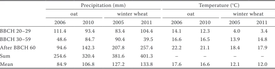
Total monthly precipitation and temperature data were provided by the Agro meteorology station at the Crop Research Institute in Prague-Ruzyně. Precipitation and temperature for observed years are also stated in Table 1.

The topographic data were obtained by using LiDAR data kindly provided by the Czech office for surveying, mapping and cadastre. Elevation data were interpolated by inverse distance weighting (IDW) in (ArcGIS 10.1) to create the DEM. The slope model (SM) and flow accumulation model (FAM) were then derived from the DEM – D8 algorithm, profile curvature (PR) and planar cur-vature (PL). TWI uses SM and FAM raster data as inputs, based on the idea that low-gradient areas will gather water (high TWI values), whereas steep

Table 1. Precipitations and temperatures at different growth stages by BBCH scale recorded in the experimental field for oat in 2006 and 2010, and for winter wheat in 2005 and 2011

Precipitation (mm) Temperature (°C)

oat winter wheat oat winter wheat

2006 2010 2005 2011 2006 2010 2005 2011 BBCH 20–29 111.4 93.4 83.4 104.4 14.1 12.3 4.0 3.4 BBCH 30–59 48.6 84.7 90.4 39.5 16.6 16.5 13.9 14.8 After BBCH 60 94.6 142.3 207.8 257.4 22.2 21.1 18.4 17.9

Sum 254.6 320.4 381.6 401.3 – – – –

convex areas will shed water (low TWI values). TWI values are non-dimensional relative indices and vary by landscape type and DEM. All topog-raphy models were created in ArcGIS 10.1 SW.

Landsat 5 TM satellite images have been provided by USGS (http://glovis.usgs.gov). The following im-age data sets were available for estimation of growth observed at the same growth stage: for oat on 13 June 2006 and 17 June 2010, and for winter wheat on 3 June 2005 and 4 June 2011. After atmospheric cor-rection of each satellite scene, the following indices were calculated: NDVI (Rouse et al. 1974), GNDVI (Gitelson et al. 1996) and MSI (Rock et al. 1985).

Pearson correlations between the yield maps, TWI, PR and PL models and indices derived from satellite imagery were assessed using the Statistica 8.0 (StatSoft Inc., Tulsa, USA) procedure at the α= 0.05 significance level. For more details see Kumhálová et al. (2011).

RESULTS AND DISCUSSION

Summary statistics of crop yield and G/NDVI (NDVI, GNDVI) and MSI are given in Tables 2 and 3. Correlation matrices between yield and the TWI, PR and PL indices were calculated for individual image data and plant species. Results of the correlation analysis are given in Table 4.

Oat and winter wheat yield had weak and nega-tive correlation with PL and posinega-tive correlation with PR. The same results were obtained for the comparison between PL/PR and G/NDVI and inversely with MSI. Guo et al. (2012) obtained similar results for the comparison of PL/PR with cotton yield and four bands in a Landsat 5 TM im-age. The types of curvature (Figure 2) indicate the directions of soil water and nutrient movement. Convex curvature is associated with soil erosion and concave curvature is with deposition (Guo et al. 2012). Theoretically, a concave area should provide more available water and nutrients sup-porting plant growth. In this study with oat and winter wheat and in another study by Guo et al. (2012) with cotton, yield was positively correlated with PR, which means that yield was higher at the convex curvature locations. Kaspar et al. (2003) stated that maize yield was negatively correlated with both curvatures, especially in dry seasons. On the other hand, Ebeid et al. (1995) reported that

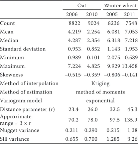
Table 2. Summary statistics of yields and methods of interpolation used for estimation of crop yields (t/ha) in selected years: 2006 and 2010 – oat, 2005 and 2011 – winter wheat

Oat Winter wheat 2006 2010 2005 2011 Count 8822 9024 8236 7548 Mean 4.219 2.254 6.081 7.053 Median 4.287 2.354 6.318 7.218 Standard deviation 0.953 0.852 1.143 1.953 Minimum 0.989 0.101 2.075 0.589 Maximum 7.224 4.825 9.929 13.458 Skewness –0.515 –0.359 –0.806 –0.141 Method of interpolation Kriging

Method of estimation method of moments Variogram model exponential

Distance parameter (r) 23.4 26.0 32.5 45.3 Approximate

range = 3 × r 70.2 78.0 97.5 135.9

Nugget variance 0.211 0.290 0.215 1.38 Sill variance 0.655 0.700 1.285 3.26

Table 3. Summary statistics of vegetation indices normalised difference vegetation index (NDVI); green NDVI (GNDVI) and moisture stress index (MSI) calculated from satellite Landsat 5 TM data acquired on respective dates

Oat Winter wheat

higher maize yield occurred at higher landscape positions, thanks to additional water stored in the clay forming the top layer of eroded soil.

Oat was grown during 2006 and 2010. There is no significant difference in correlation coefficients between the G/NDVI/MSI of individual images, yield and TWI. Correlations between MSI and all observed attributes were negative (minus) in

all years, because MSI describes the water spec-tral reflectance in growing plants (Figure 1). The year 2006 seemed to be optimal for oat growth. Oat benefited from sufficient water availability in the whole field, especially at the main growth stages. This statement was confirmed by the re-sults of summary statistics in Table 2 and by the correlation coefficients in Table 4. Oat yield was

Table 4. Correlation coefficients between the vegetation indices normalised difference vegetation index (NDVI); green NDVI (GNDVI); moisture stress index (MSI), selected topographic attributes and oat/winter wheat yields for the years 2005, 2006, 2010 and 2011. All coefficients are significant at α < 0.05

Oat Winter wheat

13. 6. 2006 17. 6. 2010 3. 6. 2005 4. 6. 2011 NDVI GNDVI MSI NDVI GNDVI MSI NDVI GNDVI MSI NDVI GNDVI MSI Yield 0.712 0.717 –0.680 0.638 0.659 –0.599 0.600 0.656 –0.651 0.764 0.752 –0.816 TWI 0.449 0.445 –0.454 0.477 0.464 –0.495 0.389 0.357 –0.419 0.387 0.366 –0.461 PL –0.151 –0.183 0.148 –0.231 –0.234 0.228 –0.099 –0.111 0.117 –0.257 –0.246 0.269 PR 0.373 0.378 –0.383 0.427 0.418 –0.463 0.226 0.188 –0.254 0.309 0.318 –0.325

Yield 2006 2010 2005 2011

TWI 0.532 0.519 0.218 0.587

PL –0.267 –0.008 –0.044 –0.251

PR 0.382 0.206 0.119 0.367

TWI – topographic wetness index; PL – planar curvature; PR – profile curvature

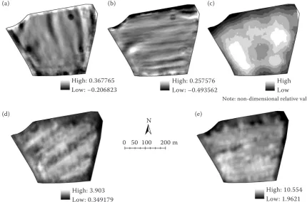
Figure 1. Maps of experimental field with planar curvature (a); profile curvature (b); topography wetness index (c); and selected maps of kriged predictions of yield (t/ha) during the observed years: 2010 – oat (d); 2011 – winter wheat (e)

(a) (b) (c)

(d) (e)

High: 0.367765 Low: –0.206823

High: 0.257576 Low: –0.493562

High Low

High: 3.903 Low: 0.349179

High: 10.554 Low: 1.9621 0 50 100 200 m

N

very low in 2010 (Table 2, Figure 2), because of intensive rainfall at the BBCH 80 growth stage, causing the crop beaten. In this year, harvesting losses caused a decrease of the yield. However, the weather conditions followed an optimum course for plant growth during the year 2010. This can be seen in Table 1 and it confirms the correlations presented in Table 4. Summary statistics in Table 3 shows that the G/NDVI spectral indices were similar in 2006 and 2010. On the contrary, the MSI values had a lower mean in 2010 than in 2006. It corresponds with more precipitation distribution on the dates of satellite data acquisition.

Winter wheat was grown in 2005 and 2011. In 2005, winter wheat benefited from sufficient water availability in the whole field, especially during the BBCH 30–59 growth stage. Correlations between G/NDVI/MSI and yield were similar to the correla-tions between these indices and those of oat. This fact most probably confirms that winter wheat was in a good condition on the dates of satellite data acquisition. Table 2 shows that winter wheat was more uniform in 2005 than in 2011. The correlation coefficient between yield and TWI (Table 4) was only 0.218. This weak correlation was caused by

high precipitation at the growth stages following after the BBCH 59 stage. On the contrary, correla-tions between G/NDVI/MSI and winter wheat yield (Figures 1 and 2) reached high values in 2011, like the correlations between yield and TWI. This crop response was probably caused by low precipita-tion during the growth stages BBCH 30–59. Low precipitation can cause a significant displacement of relatively higher yield to water-accumulating depressions. The summary statistics presented in Table 2 confirm the yield inequality, whereby both the standard deviation and min–max range were greater than in 2005. The G/NDVI/MSI values in Table 3 are in accordance with the events described.

On the basis of the presented results, it may be concluded that Landsat TM/ETM+ _{data with 30 m} resolution can be used for deriving such indices that can sufficiently explain plant variability on an 11.5 ha field at the time of data acquisition. It may be general-ly concluded that Landsat TM/ETM+ _{data with 30 m} resolution can be used for deriving such indices that can sufficiently explain plant variability. On the basis of the presented results, it may be then concluded that these indices can explain plant variability on an 11.5 ha field at the time of data acquisition. Presented

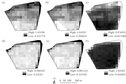
Figure 2. Maps of calculated indices – Landsat 5 TM from the dates 4. 6. 2011 for winter wheat – normalised difference vegetation index (NDVI) (a); green NDVI (GNDVI) (b); moisture stress index (MSI) (c) and 17. 6. 2010 for oat – NDVI (d); GNDVI (e); MSI (f )

(a) (b) (c)

(d) (e) (f )

High: 1.03198 Low: 0.351779

High: 1.01025 Low: 0.394653

High: 0.476935 Low: 0.0475406

High: 1.02582 Low: 0.203603 High: 0.881153

Low: 0.351595 High: 0.948245

Low: 0.32242

results further show that TWI can replace FAM and SM in explaining the influence of topography on crop yield. The relationship between TWI and yield is similar to that between yield and both FAM and SM (Kumhálová et al. 2013, Kumhálová and Moudrý 2014). Curvature was weakly correlated with all the following attributes, which was confirmed also in other studies (e.g., Guo et al. 2012).

REFERENCES

Doraiswamy P.C., Hatfield J.L., Jackson T.J., Akhmedov B., Prueger J., Stern A. (2004): Crop condition and yield simulations using Land-sat and MODIS. Remote Sensing of Environment, 92: 548–559. Doraiswamy P.C., Hollinger S., Sinclair T.R., Stern A., Akhmedov

B., Prueger J. (2001): Application of MODIS derived param-eters for regional yield assessment. In: Proceedings of Remote Sensing for Agriculture, Ecosystems, and Hydrology III, 17–21 September 2001, Toulouse, 1–8. (CD-ROM 4542-1)

Dupigny-Giroux L.A., Lewis J.E. (1999): A moisture index for surface characterization over a semiarid area. Photogrammetric Engineering and Remote Sensing, 65: 937–945.

Ebeid M.M., Lal R., Hall G.F., Mille E. (1995): Erosion effects on soil properties and soybean yield on a Miamian soil in Western Ohio in a season below normal rainfall. Soil Technology, 8: 97–108. Gitelson A.A., Kaufman Y.J., Merzlyak M.N. (1996): Use of a

green channel in remote sensing of global vegetation from EOS-MODIS. Remote Sensing of Environment, 58: 289–298. Guo W., Maas S.J., Bronson K.F. (2012): Relationship between

cotton yield and soil electrical conductivity, topography, and Landsat imagery. Precision Agriculture, 13: 678–692. Iqbal J., Read J.J., Thomasson A.J., Jenkins J.N. (2005):

Relation-ships between soil-landscape and dryland cotton lint yield. Soil Science Society of America Journal, 69: 872–882.

Jones H.G., Vaughan R.A. (2010): Remote Sensing of Vegetation: Principles, Techniques, and Applications. Oxford University Press, Oxford.

Julien Y., Sobrino J.A., Jiménez-Muñoz J.-C. (2011): Land use clas-sification from multitemporal Landsat imagery using the Yearly Land Cover Dynamics (YLCD) method. International Journal of Applied Earth Observation and Geoinformation, 13: 711–720. Kaspar T.C., Colvin T.S., Jaynes D.B., Karlen D.L., James D.E., Meek

D.W., Pulido D., Butler H. (2003): Relationship between six years of corn yields and terrain attributes. Precision Agriculture, 4: 87–101. Kumhálová J., Kumhála F., Kroulík M., Matějková Š. (2011): The

impact of topography on soil properties and yield and the ef-fects of weather conditions. Precision Agriculture, 12: 813–830.

Kumhálová J., Kumhála F., Novák P., Matějková Š. (2013): Air-borne laser scanning data as a source of field topographical characteristics. Plant, Soil and Environment, 59: 423–431. Kumhálová J., Moudrý V. (2014): Topographical characteristics

for precision agriculture in conditions of the Czech Republic. Applied Geography, 50: 90–98.

Marques da Silva J.R., Silva L.L. (2006): Relationship between distance to flow accumulation lines and spatial variability of irrigated maize grain yield and moisture at harvest. Biosystems Engineering, 94: 525–533.

Marques da Silva J.R., Silva L.L. (2008): Evaluation of the relationship between maize yield spatial and temporal variability and different topographic attributes. Biosystems Engineering, 101: 183–190. Momm H., Bingner R., Wells R., Rigby J., Dabney S. (2013):

Ef-fect of topographic characteristics on compound topographic index for identification of gully channel initiation locations. Transactions of the ASABE, 56: 523–537.

Murphy P.N.C., Ogilvie J., Arp P. (2009): Topographic modelling of soil moisture conditions: A comparison and verification of two models. European Journal of Soil Science, 60: 94–109. Nigon T.J., Mulla D.J., Rossen C.J., Cohen Y., Alchanatis V., Rud

R. (2014): Evaluation of the nitrogen sufficiency index for use with resolution, broadband aerial imagery in a commercial potato field. Precision Agriculture, 15: 202–226.

Pilesjö P., Thylén L., Persson A. (2005): Topographical data for deline-ation of agricultural management. In: Stafford J.V. (ed.): Precision Agriculture. Wageningen Academic Publishers, Uppsala, 819–826. Rock B.N., Williams D.L., Vogelmann J.E. (1985): Field and air-borne spectral characterization of suspected acid deposition damage in red spruce (Picea rubens) from Vermont. In: Pro-ceedings: Symposia on Machine Processing of Remotely Sensed Data, Purdue University, West Lafayette, IN, 71–81.

Rouse J.W., Haas R.H., Schell J.A., Deering D.W. (1974): Moni-toring vegetation systems in the Great Plains with ERTS. In: Proceedings Third ERTS-1 Symposium, NASA Goddard, NASA SP-351, 309–317.

Serrano J.M., Shahidian S., Marques da Silva J.R. (2013): Small scale soil variation and its effect on pasture yield in southern Portugal. Geoderma, 195–196: 173–183.

Schmidt F., Persson A. (2003): Comparison of DEM data capture and topographic wetness indices. Precision Agriculture, 4: 179–192. Sørensen R., Zinko U., Seibert J. (2006): On the calculation of

the topographic wetness index: Evaluation of different meth-ods based on field observations. Hydrology and Earth System Sciences, 10: 101–112.

Zhang Q., Pierce J.F. (2013): Agricultural Automation: Funda-mentals and Practices. CRC Press, Boca Raton.

Received on June 20, 2014 Accepted on September 19, 2014

Corresponding author:

Mgr. Jitka Kumhálová, PhD., Česká zemědělská univerzita v Praze, Fakulta životního prostředí, Katedra aplikované geoinformatiky a územního plánování, Kamýcká 129, 165 21 Praha-Suchdol, Česká republika