Appearance of Negative Differential Conductivity in Graphene Nanoribbons at High Harmonics

Appearance of Negative Differential Conductivity in

Graphene Nanoribbons at High-Harmonics

Musah Rabiu1, Samuel Y. Mensah2, Sulemana S. Abukari2 1_{Department of Applied Physics, University for Development Studies, Navrongo, Ghana} 2_{Physics Department, Center for Laser and Fiber Optics, University of Cape Coast, Cape Coast, Ghana}

Email: [email protected]

Received February 8, 2013; revised March 11, 2013; accepted April 3, 2013

Copyright © 2013 Musah Rabiu et al. This is an open access article distributed under the Creative Commons Attribution License,

which permits unrestricted use, distribution, and reproduction in any medium, provided the original work is properly cited.

ABSTRACT

We theoretically study current dynamics of graphene nanoribbons subject to DC-AC driven fields. We show that gra- phene exhibits negative differential conductivity (NDC) at high-harmonics. NDC occurs in the neighborhood where a constant electric field is equal to amplitude of ac field. We also observe NDC at both even and odd harmonics and at wave mixing of two commensurate frequencies. The even harmonics are more pronounced than the odd harmonics. A possible use of the present method for generating terahertz frequencies at even harmonics in graphene is suggested.

Keywords: Graphene Nanoribbon; Energy Spectrum; Electronic Conductivity; Terahertz;

Negative Differential Conductivity

1. Introduction

Graphene has attracted much attention since its discovery in 2004 by Geim and his team [1]. The great interest in studying graphene is driven by its unique band structure [2] and many unusual physical properties like electrical, ther- mal and mechanical properties [3]. Despite these, there have been difficulties in realizing graphene-based elec- tronic devices, probably, the fact that the graphene sheet lacks band gap, edge defects, disorder, etc. However, various attempts have been made to introduce 2D gra- phene sheet, for the purpose of overcoming some of these challenges, into a 1D + quantization. This phenomenon results into graphene nanoribbon (GNR) which is assum- ed as an unrolled single-wall carbon nanotube (SWCNT). Depending on the nature of the nanoribbon edges, one gets two symmetry groups; armchair graphene nanoribbon (aGNR) and zigzag graphene nanoribbon (zGNR). Arm- chair and zigzag GNRs show metallic or semicon-ducting electronic properties [4] depending on the number of dimer rows,  along transverse direction.  is related to the width of the nanoribbon as  3





Dirac fermions can reach the edges within a femto-second before encountering any lattice effects, and avoiding ele- ctron-electron interaction, eletron-phonon interaction, etc. In this paper, we employ Boltzmann transport equation based on relaxation time approximation to study negative differential conductivity (NDC) in GNRs. In conventional semiconductor devices including semiconductor super- lattices, an NDC behavior is known to offer great potential for high frequency applications as Bloch oscillators, fre- quency multipliers, and fast switching devices. For this reason, the NDC effect has been greatly explored and discussed in several graphene nanostructures, particularly in [7]. NDC can also be observed in other graphene allo- tropes; carbon nanotubes (CNT) [8]. The unique energy spectrum of holes and electrons in GNRs, especially its narrow gap nature leads to nontrivial features such as NDC in the THz regime [7].

The rest of this paper is organized as follows; In Sec-tion 2, we derived the electronic current density of aGNR and zGNR and imposed certain conditions to reduce the equations to forms appropriate for our model. The results obtained in Section 3 are discussed in great details in Section 4. The paper finally concludes in Section 5 where some recommendations for future applications are made.



1 2

2. The Theory

Following the approach of refs, [8,9] for SWCNT and semiconductor superlattices, we consider an undoped GNR (both zigzag and armchair) exposed simultaneously to DC AC electric field

 

i 

0 e

jt j n

j j

E t 



_ E   , (1) which is seen as a superposition of n harmonic waves po-

larized along one direction with angular frequency. The phase difference between the



j1



th and th compo-

nent being j1 j

j

    is arbitrary, is an integer. are the field amplitudes. We require that

0 0

j

j

E

0

   . This will correspond to the DC component of the applied field. The dynamics of free -electrons in graphene can be describe by the time-dependent Boltz-mann transport equation (BTE) based on relaxation time approximation in zero magnetic field as

π

 

   

_{ }

_{ }

0

, ,

Γ , .

f k t eE t f k t

f k t f k

t k

 

  _  _

 _  (2)

We also assume a spatial uniform graphene nanorib-bon. Again, the inverse of the relaxation time is momentum independent. In Equation (1),

Γ

 

0

f k and

 

,

f t k are the equilibrium and non-equilibrium Fermi electron distribution functions, respectively. e is the

electronic charge, is the electron wave vector and is the reduced plank constant. In the following section, we will calculate electronic current density for GNRs.

k _

2.1. Armchair and Zigzag Nanoribbon Band Structures

The energy band structure of aGNR and zGNR is charac- terized by three parameters; band index , phase  and wave vector k [5,6]. For aGNR,

 

2







  

0

, 1 4 cos 4cos cos kl ,

k s s

 _{     }



(3) and for zGNR,

 

2

 



  

0

, 1 4 cos 4 cos cos

k kl s k .

 _{      l}

 (4)

where  1 with (+) for conduction band and (−) for valence band. l 3 2a and l a 2, is the lat-tice spacing which has numerical value of 0.246 nm,

0

a

~ 3.0 eV

 is the overlap integral and  is the phase perpendicular to the quasi-momentum . The 1 BZ of aGNR is bounded by

k





π2,π 2



kl  and the zGNR is

 

0,π k

s

kl  . is parallel to the edge and has transla- tional symmetry along this direction. For aGNR, the transverse wave vector (phase) is quantized according to the rule [6]  sΔ with Δ π



 1



and

1, 2

s , ,  . Unlike aGNR, the nature of transverse wave vector quantization is complicated in zGNR,

de-pending on both k and  as

 









Δs πjΛ k,  1 . However, for simplicity we assume Λ is constant, say π 2, so that













Δ s 2j1 π 2  1 . Except this little subtlety for zGNRs, all that will be discussed in the following for aGNR are equally applied to the zGNR.



Now, we employed the translational invariance of gra- phene ribbon in the reciprocal space and expand in Fou- rier series functions f f, 0 and  along the edge hav- ing periodicity in k. i.e.,

 

 

irkl

r f   0 f k 0 , r   e ,



(5)



_{, ,}



 

_eirkl_Φ



_,

r r



f k  t f  t

0 r





(6)

 

, 0

r   

 

i 0 rkl r  

k



e .

  (7)

The Fourier coefficient fr is expressed as

 

1 sΔ



s



r s r

f  



_ f   sΔ with

 

π2 _i

0

π2 d , e ,

π Δ

l _rkl

rs _l rs rs

l

f k f k f f

s 

 

 _ 



_

 (8)

and

 

π2 _i

0

k f

π2 d , e ,

π

l _rkl

r _l r r

l

k  _

 

  

0





 . (9)

2

s

In (6), counts the number of dimers  in the GNRs. The factor in the equation is a central point in this paper and so has to be determined. is an inte-ger and not equal to zero. We consider a classical limit in which energy levels could be excited due to thermal fluctuations, i.e.

Φr

r

Δ BT C. This condition is also necessary for large enough field, so that charge carriers can escape low energy scattering [10]. The energy level spacing

K

 

0 W l

Δπ  A, _C is the charging energy, B

k W

is Boltzmann constant, is lattice temperature and is the graphene nonoribbon width. In what follows, we will compute

T

 

Φ t . To do this, (5), (6) and (7) are

substituted in (1) following the simplification scheme

1, 2

j j ,3,_ and . We ob- tained

, 1

j j   , 2, 3,

m n

 

 

 

i

_

i

_

, 1

n

r t Jn





. n m 0 e Φ . 1 i

j j j j

j j j

t

j n j

n j j j

J                   j j j  



j j (10) where   

2.2. Sheet Current Density

The sheet current density of graphene can be determined from the relation

 

s s .

k k k

g g

A

the sheet area A WL . g_s, g_v are the spin and valley degeneracies, respectively. The current density can also be written as

 

2



 

r

1

d , , ,Φ . 4π

s v

s s

s

g g e

j t kv k f k











(12)

the velocity of Dirac fermions in graphene is defined as

 

v k   k. In terms of the Fourier coefficients,

 

0 i

0

i

, rkl

r r

l v k  







 e

.

(13)

Giving

 

0,

 

1

i r r r

j t j t c c









  (14)

with

0

0, 0, 0,

1

2 _{Δ ,}

π

s v

r rs rs r

s

g g e

j f j

l

 _  _.

r

j _







 

  

Note the dependence of r j, 0 and the summa- tion over the index in (10). Using the formalism by Lit-vinov and Manasson [9]. Equation (14) can be put in a Taylor-like expansion in terms of Ej. i.e.,

i

0

1

. e . 2

j j

j j j

t

DC j n

j

j j E _ c c  







 

     

 



 

  (15)

where

 



0



2

0, 2

1 1

0 i

. 1

j

n

j j

DC r n j

r j

j j

n

j j J

n

    

  

 

  

 

 

 

_  _

 

c c (16)

is the differential DC current density (for _j 0), and

 

 





0,

1 1

0

2 0

2

i

e 1

j j j

j j

j

j j n

n j n j

n r

r n j j

v j j

j j

J J

j

E

n

n

 



 



   

  

  _

  



 



 

_  _



 

(17)

is the large-signal dynamic nonlinear conductivity at j

harmonic with drive frequency _j.

3. Negative Differential Conductivity

3.1. Pure DC Limit

To see immediately that (16) demonstrates NDC, we consider a pure DC limit where j 0

 

. The Bessel functions except the term will vanish. The real part of the differential conductivity

0

n

0 0

im

j j E

 

  

0 l  become

 

 

 

2 0

0, ₂ 2

1

0

1 0

1

r r

el  

 

 





 

So that if 1

0 ,

 _ _{the differential conductivity is}

negative and NDC is manifest in GNRs. Electron dyna- mics may be come more complicated in the presence of high-frequency components in addition to the static elec-tric fields. High negative differential conductivity thus may result in GNRs if an external drive force is applied.

3.2. Monoharmonics

If one component of the AC field in (2) is applied, then

1

n and (16) simplifies to

 





2 0 1

0, 2

0 1

, 1

r n r n

n

j j J

n

    

  





 

 

_  _

 

(19)

after dropping the subscript on Here, it not clear im-mediately how NDC can be seen. To observe the phe-nomenon, we plot with 0 for

.

n

j E  1 as shown

in Figure 1 (top) for armchair ribbon and in Figure 1

(buttom) for zigzag ribbon,

.

 _ 

 



[image:3.595.54.288.184.307.2]

 (18)

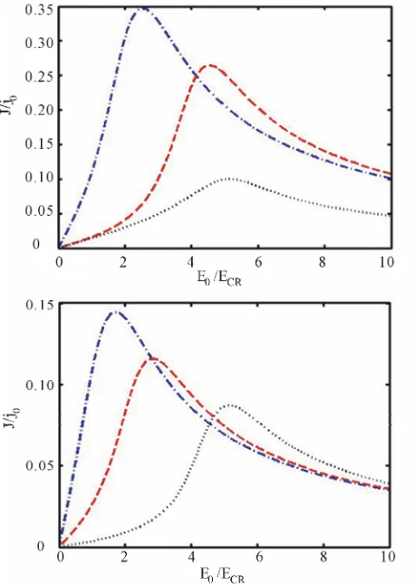
[image:3.595.308.537.331.654.2]

The effect of NDC is strong in zigzag graphene than in armchair graphene. Especially, in the limit of high har- monic field, NDC is greatly suppressed in aGNR.

3.3. Biharmonics

In practical situations, one can also allow graphene nano- ribbon subject to two AC field components. In that case, we let in our general formalism in Section 2. Equation (15) takes the form

1, 2

j

 

 

 

 

_

_

1 1 1 1 2 1 2

1 1 2 2

2 2 2

0, 1 1

1 , ,

i i

2 2

0 1 1 2 2

i

e

, 1 i

r n n

r n n

n n

j j J J

J J

n n

  

    

 

 

   

  

   

 





  



 

(20)

and from which (17) follows. We have eliminated the time dependence by averaging over the period of the fields to find the time-independent current . In the left hand side, we replaced

j

 

j t  j, and in the right hand side a delta function emerges which ensures that 1 



  2 1



2

2

. If 1

  , then one must put 10 and 2 so that

1 2

  . However, we shall generalize this to a case of commensurate frequencies. We exemplified the case by a biharmonic having frequencies which can be periodic

2 1

  or non-periodic, 21 with 1, 2, . These two cases were studied in [11,12] for semiconduc- tor superlattices. Simplifying further, we linearize with respect to one of the field amplitudes (say, ). For a week field, 2

2 E

1

 and Jn

  

   2



2 n!, which allows us to take n n₂



₂₂



1 0,



1



. Finally, the

AC current density becomes





 



 

 

2

0

2 0, 2

1 ₀

1 ?

cos

1

– .

r r

n n n

n el

j E j

n

J r J _ r J _ r

  

 _





  

  







 

 





 (21)

1,2 erlE1,2 1,2

  _ . Equation (21) reduces to the mono- harmonic case when 1.

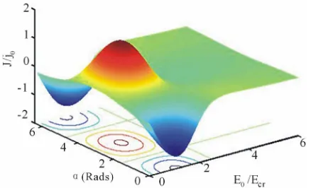
The nature of the NDC is observed for a simultane- ously varying harmonic field and phase difference in a three dimensional plot shown in Figure2.

4. Discussion and Conclusions

In Figure 1 normalized current density j j0 is plotted

against reduced static electric field E0 Ecr for aGNR (left) and zGNR (right) for an applied field. At low fields up to , the quantum derivative of the 0 characteristic yields a positive slope. A negative slope results for

AC DC



0 max

E j





jE



0 0

E E j_max . In the whole region,





0 0

E E _max graphene nanoribbon device will operate under Negative Differential Conductivity (NDC). A consequence of NDC in GNR is a formation of electric

field domains that impedes a continuous motion of elec-trons generated by the external electric field and thus blocks high frequency oscillations in the nanoribbon. NDC disappears quite faster in aGNR as com-pared to zGNR which is more rubust at this limit.

j

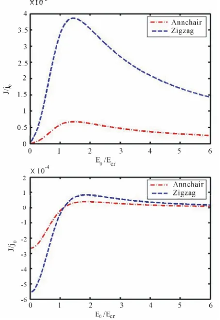
E  The curves in Figure 3 demonstrate NDC phenomenon.

They are obtained at wave mixing of two commensurate frequencies, 21. Figure 3 (left),  odd and

Figure 3 (right), even. The onset of NDC in odd-

harmonics occurs around 0 1 and in even-har- monics it starts at

~ ,

E E

0

E E₁. In both cases, as in the pre-vious NDC graphs,  1.

The combined effect of phase shift , between two AC fields and amplitude on NDC is depicted in Figure 2.

There are three peaks at low bias fields at points



EEcr,0



,



EEcr,π



0, 2π,

and .

It is not very clear what these crests and troughs mean, they might be associated with field domains along one direction (for



EEcr, 2π



  _

π,3π,

) and others along the opposite direction (for  _) and vice-versa. This means

that electron velocity is higher in the domain with the same polarization along the electron direction and lower in the domain with opposite polarization.

In conclusion, we have demonstrated that graphene nanoribbons exhibit NDC regions in its 0 charac-teristics at low bias field when

jE

1

 . NDC is observed either in the presence of bias field alone or by superim- Posing AC fields on the bias field. For one AC field component, NDC occurs around 0.1

0.

. When two AC fields at commensurate frequencies are applied, high- harmonic NDC emerge for both even and odd harmonics at rather very low frequencies   01. The even-

series gives pronounced high-harmonic NDC than the

odd-series. The presence of high-harmonic NDC means

that it is possible for high-frequency generation in gra- phene nanoribbons when electric field domains are sup- pressed at high enough applied frequencies  1

andE0Ecr. We therefore suggest this approach for the

[image:4.595.315.534.560.693.2]

[3] R. S. Shishir and D. K. Ferry, “Intrinsic Mobility in Gra- phene,” Journal of Physics: Condensed Matter, Vol. 21, No. 23, 2009, Article ID: 232204.

doi:10.1088/0953-8984/21/23/232204

[4] L. Brey and H. A. Fertig, “Electronic States of Graphene Nanoribbons,” Physical Review B, Vol. 73, No. 23, 2006,

Article ID: 235411.

[5] F. Hipolito, A. H. Chaves, R. M. Ribeiro, M. I. Vasilev- skiy, V. M. Pereira and N. M. R. Peres, “Enhanced Opti- cal Dichroism of Graphene Nanoribbons,” Physical Re- view B, Vol. 86, No. 11, 2012, Article ID: 115430.

doi:10.1103/PhysRevB.86.115430

[6] K. Sasaki, K. Kato, Y. Tokura, K. Oguri and T. Sogawa, “Theory of Optical Transitions in Graphene Nanorib- bons,” Physical Review B, Vol. 84, No. 8, 2011, Article

ID: 085458. doi:10.1103/PhysRevB.84.085458

[7] V. Ryzhii, M. Ryzhii and T. Otsiji, “Negative Dynamic Conductivity of Graphene with Optical Pumping,” Jour-nal of Applied Physics, Vol. 101, No. 8, 2007, Article ID:

083114. doi:10.1063/1.2717566

[8] S. S. Abukari, S. Y. Mensah, K. W. Adu, N. G. Mensah, K. A. Dompreh, A. Twum, C. L. Y. Amuah, M. Amek- pewu and M. Rabiu, “Domain Suppression in the Nega- tive Differential Conductivity Region of Carbon Nano- tubes by Applied AC Electric Field,” World Journal of Condensed Matter Physics, Vol. 2, No. 4, 2012, pp. 274-

277. doi:10.4236/wjcmp.2012.24045

[9] V. I. Litvinov and A. Manasson, “A Large-Signal Nega- tive Dynamic Conductivity and High-Harmonic Oscilla- tions in a Superlattice,” Physical Review B, Vol. 70, No. 19, 2004, Article ID: 195323.

[image:5.595.59.286.91.421.2]

doi:10.1103/PhysRevB.70.195323 Figure 3. Negative differential conductivity due to wave

mixing of two AC field amplitudes. (top) even and (buttom) odd . The parameters used are E10.2Ecr,

cr

E₂E and  0.01.

[10] S. K. Sekwao and J. P. Leburton, “Hot Electron Terahertz Oscillations in Graphene: Crater and Terraces in the Car-rier Distribution Function,” Preprint, arXiv:1003.0842v1. [11] K. A. Pronin and A. D. Bandrauk, “Coherent Control of

Electric Currents in Superlattices and Molecular Wires: Effect of Relaxation,” Physical Review B, Vol. 69, No. 19, 2004, Article ID: 195308.

doi:10.1103/PhysRevB.69.195308 study of terahertz generation in graphene.

REFERENCES

[12] K. Seeger, “High-Frequency-Induced Phase-Dependent DC Current by Bloch Oscillator Non-Ohmicity,” Applied Physics Letters, Vol. 76, No. 1, 2000, pp. 82-84. doi:10.1063/1.125663

[1] K. S. Novoselov, A. K. Geim, S. V. Morozov, D. Jiang, Y. Zhang, S. V. Dubonos, I. V. Grigorieva and A. A. Firsov, “Electric Field Effect in Atomically Thin Carbon Films,”

Science, Vol. 306, No. 5696, 2004, pp. 666-669.

doi:10.1126/science.1102896

[2] K. S. Novoselov, A. K. Geim, S. V. Morozov, D. Jiang, M. I. Katsenelson, I. V. Grigorieva, S. V. Dubonus and A. A. Firsov, “Two-Dimensional Gas of Massless Dirac Fer- mions in Graphene,” Nature, Vol. 438, No. 7065, 2005, pp.