Munich Personal RePEc Archive
Mortgage Lending and the Great
moderation: a multivariate GARCH
Approach
Bezemer, Dirk J and Grydaki, Maria
University of Groningen
January 2012
Online at
https://mpra.ub.uni-muenchen.de/36356/
1
MORTGAGE LENDING AND THE GREAT MODERATION:
A MULTIVARIATE GARCH APPROACH
Dirk Bezemer and Maria Grydaki*
Faculty of Economics and Business, University of Groningen, The Netherlands
February 2, 2012
Abstract
Financial innovation during the Great Moderation increased the size and scope of credit flows in
the U.S. Credit flows increased both in volume and with regard to the range of activities and
investments that was debt-financed. This may have contributed to the reduction in output
volatility that was the Great Moderation. We hypothesize that during the Great Moderation (i)
growth in mortgage finance partly decoupled from fundamentals as measured by overall output
growth and (ii) this allowed mortgages less to finance residential investment and more to finance
spending on other GDP components. We document that the start of the Moderation coincided
with a surge in bank credit creation (especially mortgage credit), a rise in property income, a rise
in the consumption share of GDP, and a change in correlation (from positive to negative)
between consumption and non-consumption GDP components (investment, export and
government expenditure). In a multivariate GARCH framework, we observe unidirectional
causality in variance from total output to mortgage lending before the Great Moderation, which
is no longer detectable during the Great Moderation. We also find that bidirectional causality in
variance of home mortgage lending and residential investment existed before, but not during the
Great Moderation. Both these findings are consistent with a role for credit dynamics in
explaining the Great Moderation.
Key Words: great moderation, mortgage credit, multivariate GARCH, causality
JEL codes: E44, C32, C51, C52
*
We share equal authorship. E-mail addresses: d.j.bezemer@rug.nl (Dirk Bezemer, corresponding author),
2
1. Introduction
A substantial literature addresses the dramatic decline in macroeconomic volatility of the U.S.
economy between the mid-1980s and the start of the 2007 financial crisis (Kim and Nelson
1999)1. Warnock and Warnock (2000) documented strongly declining employment volatility.
Blanchard and Simon (2001) noted declines in the standard deviation of quarterly growth and
inflation by half and by two thirds, respectively, since 1984. Stock and Watson (2002) found that
the standard deviation of U.S. GDP declined from 2.6 - 2.7% in the 1970s and 1980s to 1.5% in
the 1990s. Bernanke (2004) drew broad attention to these trends by making it the topic of his
2004 Eastern Economic Association speech. Many countries, particularly the Anglo-Saxon
economies, shared this feature. Cechetti and Krause (2006) find that in sixteen out of twenty-five
countries they examined, real GDP growth was on average more than fifty per cent less volatile
than it was twenty years earlier to their study.
Some writers argue that the greater stability signified that the U.S. economy entered a new
phase around 1984. The name ‘Great Moderation’, reminiscent of America’s Great Depression
and Great Inflation episodes, conveys this sense of a new era. The novel element is variously
thought to be better inventory management (McConnell and Perez-Quiros, 2000; Kahn et al.,
2002; McCarthy and Zakajsek, 2007), fundamental labour market changes as the Baby Boomer
generation is aging (Jaimovic and Siu, 2009), oil shocks (Nakov and Pescatori, 2010),changes in
responses to shocks (Gambetti et al., 2008) or broader factors such as development levels
(Acemoglu and Zilibotti, 1997; Easterley et al., 1993), external balances (Fogli and Perri, 2006),
the size of the economy (Canning et al., 1998) and lack of strong institutions (Acemoglou et al.,
2003). Owyang et al. (2007) find that within U.S. states, the volatility decline was linked to
larger nondurable-goods shares, energy consumption, and demographics. Other analysts point to
the role of chance and suggest that the volatility decline may well be due to smaller or less
frequent shocks to the economy, quite outside the influence of policy makers – or ‘good luck’
(Ahmed et al., 2002; Cogley and Sargent, 2005; Primeceri, 2005; Sims and Zha, 2006;Gambetti
et al., 2008). Benati and Surico (2009) show that most analyses, which use Structural Vector
Autoregression (SVAR) models, are compatible with both ‘good policy’ and ‘good luck.’
3 A number of papers pursue a ‘financial sector’ explanation of the Great Moderation. These
revolve around financial innovations (Dynan et al., 2006; Guerron-Quintana, 2009), financial
sector development (Easterly et al., 2000), changing responses to monetary shocks and
improvements in monetary policy (Clarida et al., 2000; Bernanke, 2004; Lubik and Schirfheide
2004; Boivin and Giannoni, 2006), and innovations in financial markets and in the dynamics of
inflation (Blanchard and Simon, 2001). A common outcome of many of these developments is
increased liquidity, though the reasons vary from monetary policy to trade integration to
financial stability. For instance, Bean (2011) discusses how the volatilities of both U.S. equities
and treasuries had shrunk to very low levels by the mid-2000s, and quotes the Dynan et al.
(2006) explanation of how financial innovation smoothed financial variables (such as returns on
financial assets). This signalled (correctly or falsely) low risk levels to both banks and real-sector
actors, encouraging them to lend and borrow more, respectively.
In the present paper we contribute to this literature. Financial innovation during the Great
Moderation increased credit flows in the U.S. both in volume and with regard to the range of
activities and investments they financed. We hypothesize that more of economic activity was
debt-financed during the Great Moderation than before, and that those debt-financed incomes
moved more independently from overall GDP, leading to a reduction in overall output volatility.
We refer to this hypothesis as the ‘credit-driven Great Moderation hypothesis’ (or CDGM
hypothesis, for short).
Specifically, we hypothesize that during the Great Moderation (i) growth in mortgage
finance partly decoupled from fundamentals as measured by overall output growth and (ii) this
allowed mortgage less to finance residential investment and by implication, more to finance
spending on other GDP components2. Below we document that the start of the Moderation
coincided with a surge in bank credit creation (especially mortgage credit), a rise in property
income, a rise in the consumption share of GDP, and a change in correlation (from positive to
negative) between consumption and non-consumption GDP components (investment, export and
government expenditure). In a multivariate Generalized Autoregressive Conditional
2
4 Heteroskedasticity (GARCH) framework, we observe unidirectional causality in variance from
total output to mortgage lending before the Great Moderation, which is no longer detectable
during the Great Moderation. We also find that bidirectional causality in variance of home
mortgage lending and residential investment existed before, but not during the Great Moderation.
Both these findings are consistent with a credit-driven Great Moderation, in conjunction with the
other explanations discussed above.
Importantly, we test these relations in variances rather than levels. The Great Moderation
was a reduction in the variance of output (denoted Y), but also of the financial-sector variables
that possibly caused it (Bean, 2011). We therefore study also the variances (not only the levels)
of mortgage lending (denoted M) and residential investment (denoted RI). An intuitive way to
see the importance of the causality-in-variance approach in this paper is to decompose output
into residential investment and other GDP components so that Y=RI+(Y-RI) and
var(Y)=var(RI)+var(Y-RI)+2cov(RI,Y-RI). Financial innovation may reduce var(Y) by reducing
any one of the three right-hand terms of this expression. A VAR analysis in terms of levels only
(e.g. Den Haan and Sterk, 2010) captures the first channel but not the second and third. And
since this first channel is the least likely one, it is unsurprising that this method finds no evidence
for the financial sector view of the Great Moderation3. By testing directly for var(Y), var(M) and
var(RI) we capture all three possible channels, including (importantly) their covariances. We do
this below in a multivariate GARCH framework.
The remainder of the paper proceeds as follows. In the next section we explore relevant
trends in the U.S. economy and locate the argument in the literature. Section 3 develops the
methodology and section 4 presents the data as well as the estimation and test results. Section 5
concludes with a summing up and discussion.
3
5
2. Locating the Argument: Empirical Trends and Relevant Literature
2.1. Some Trends
In this section we present and discuss six developments consistent with our hypothesis, and then
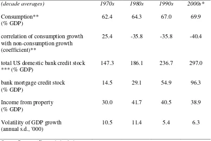
locate it in the literature (Table 1; all data are taken from the Bureau of Economic Analysis).
[Table 1 HERE]
The average annual volatility of GDP growth nearly halved from 0.0105 in the 1970s and 0.0114
in the 1980s to 0.006 over 1984-2007 – the key feature we attempt to explain, and which is also
widely documented in other places (e.g. Bean, 2011). The share of consumption in GDP, which
had been virtually stable between 60% and 63% from 1953 to 1981, rose from 64% in 1982 to
70% in 2000-2007. Historically, this was a rapid increase. It implies that the importance of any
factors driving consumption (such as mortgage lending) also became more relevant to
understanding GDP and its volatility. Shocks to the investment, export and government
expenditure components of GDP were increasingly counterbalanced by private consumption
movements in opposite direction. The correlation coefficient between the two (in differenced
growth rates) was positive (+0.25) in the 1970s but turned negative (-0.36 to -0.40) from the
1980s onwards. Significantly, most of that decline occurred around the start of Great Moderation
in the mid-1980s. For most of the Great Moderation years, declines in the combined investment,
net export and government expenditures components of GDP were balanced by increases in
private consumption.4 This is consistent with the view that variations in private consumption
cushioned negative movements to the other, non-consumption GDP components, reducing the
volatility of total output.
The liquidity that facilitated the increase in consumption was provided by increases in the
total bank credit stock, which doubled in relative terms from 1.5 times GDP in the 1970s to 3
times GDP in the 2000s. The rise in bank credit creation was largely due to the most important
category of credit in the domestic U.S. economy, the stock of mortgage credit. This rose from
4
6 just 3% of GDP in the early 1950s to 30% of GDP in 1985 and on to an average 96% in the
2000s. Other credit stocks also increased, especially in the Great Moderation, but more slowly.
This shift in credit flows is linked to the rise in income from property as a share of GDP:
from 30% in the 1970s to around 40% in the 1980s, 1990s and 2000s. Again, most of that
increase occurred at the start of the 1980s. In the four years 1978-1982, income from property
rose from 31% to 42% of GDP. Then it remained at that level, fluctuating between 35% and 45%
for the remainder of the Great Moderation. This trend was also evident in the estimated housing
wealth effect on consumption. Carroll et al. (2006) estimate that in the U.S. over 1960-2004, the
immediate (next-quarter) marginal propensity to consume from a $1 change in housing wealth
was about two cents, increasing to around between four and ten cents in the long run. During the
Great Moderation, average nominal U.S. house prices more than tripled, so that the housing
wealth effect would have induced an increase of consumption of 12 to 30 per cent over the
period (in nominal values). To the extent that wealth-induced consumption was countercyclical
to other GDP components, this could lead to significant GDP smoothing. These figures are only
indicative, but the orders of magnitude are sufficiently large that the distribution of these gains
over time will matter to the volatility of GDP.
2.2. Relevant Literature
The CDGM hypothesis fits into the Great Moderation literature. For instance, Gambetti et al.
(2008) find changes in the way the private sector responds to supply and real demand shocks,
together with changes in the variability of structural shocks. A next step is to research why
responses changed; altered availability of credit is one possible reason. Beyond the Great
Moderation literature, the present paper also connects to a strand of literature where credit is a
key factor in understanding the macroeconomy, especially cyclicality and volatility (Bernanke,
1993; Bernanke and Blinder, 1998; Bliss and Kaufmann, 2003). While most contemporary work
on credit and the macroeconomy is in the spirit of the Credit View (Bernanke and Gertler, 1995)
or some variety of an accelerator model (Kyotaki and Moore, 1997), the present emphasis is on
the more traditional notion of credit as the prime source of liquidity, enabling agents to finance
expenditures (as also in Borio and Lowe, 2004). This paper follows the Kocherlakota (2000)
7 argument that looser credit policies can create stability. It, thus, also connects to the literature
which views business cycles (partly) as credit cycles (Kiyotaki and Moore, 1997; Mendicino,
2007). In support, Benk et al. (2005), building on Uhlig (2004), identify credit shocks as
candidate shocks that matter in determining GDP.
We explore linkages between (the volatility of) credit components and GDP components.
These linkages are supported by Caporale and Howells (2001) who analyse the interactions
between bank loans, bank deposits and total transactions in the economy. They conclude that
“loans cause deposits and that those deposits cause an expansion of wealth/GDP transactions”
(Caporale and Howells, 2001:555). This paper is also focused on loan volumes rather than
interest rates; Lown and Morgan (2006) show that loan volumes – determined largely by credit
standards and regulation – dominate loan rates in explaining output and output components.
Their work also suggests that the CDGM hypothesis is complementary (rather than rival) to the
well established inventory explanation (McConnell and Perez-Quiros, 2000; Kahn et al., 2002;
McCarthy and Zakajsek, 2007). The Lown and Morgan (2006) VAR analysis suggests a large
impact of weakening of loan on declining inventory investment. This suggests that the widely
noted decline in loan standards during the Great Moderation led to both declining inventory
investment and to more mortgage lending. Both, in different ways, may have contributed to
declining output volatility. Other closely related papers outside the Great Moderation literature
are by Campbell (2005), who poses a link between rapid growth and increased volatility in credit
flows to financial markets and stability in the real economy. Also, Lorrain (2006) finds that the
volatility of industrial output is lower in countries with more bank credit.
Den Haan and Sterk (2010) address another interpretation of the CDGM hypothesis in a test
for structural breaks in the relation between mortgage lending and consumption in the U.S. in a
SVAR specification– but in levels, not variances. They find no evidence of breaks and reject the
hypothesis that financial innovation caused the Great Moderation. Another relevant finding is by
Davis and Kahn (2008), who decompose the decline in macro volatility and find that most of it is
explained by a combination of changes in firm-level volatility and aggregate volatility – most
clearly in the durable goods sector. A surprising finding in their study is that both volatility
declines occurred without a decline in the volatility of household consumption, or in the
uncertainty of incomes. Davis and Kahn (2008) therefore ascribe the lower durable goods sector
8 better supply chain management (especially, inventory control) and a shift from employment and
production from goods to services. However, both these studies consider the level, but not the
variance of real output and its financial-sector determinants. This is where we break new ground.
Even if the volatility of household consumption did not decline as Davis and Kahn (2008) report,
if its covariance with other GDP components turned form positive to negative (Table 1) that
would reduce output volatility.
3. Methodology
3.1. Modeling Volatility
In this section we present our econometric model and approach. To model conditional variances
and covariances we estimate a multivariate GARCH model, an extension of a univariate GARCH
model (Bollerslev, 1986 based on Engle’s (1982) ARCH model). We first test for the existence
of ARCH effects or volatility clustering, which is the tendency of large (small) changes (of either
sign) to follow large (small) changes and, so that current and past volatility levels tend to
correlate positively. In the presence of ARCH effects we proceed with the estimation of a
multivariate GARCH model. Of the several possible specifications for multivariate GARCH
models5 we choose an unrestricted bivariate VAR-BEKK model (Engle and Kroner, 1995),
appropriate for the computation of conditional variances and covariances between variables6.
Below we discuss the VAR-BEKK model in terms of two variables, home mortgages and either
real output or residential investment. This implies two conditional mean equations. We choose a
GARCH (1,1) model for the conditional variance specification because it is more parsimonious
than ARCH, avoids over-fitting and is usually sufficient to capture volatility clustering
(higher-order model are rarely estimated in the academic finance literature). We test for bidirectional
causality of the conditional variance of home mortgages growth with the conditional variance of
output growth and of residential investment. Here we go.
5
A common specification of multivariate GARCH models is the VECH model (Bollerslev et al. 1988), which seems infeasible to be estimated because of the large number of parameters. To solve this, Bollerslev et al. proposed the diagonal VECH, but this does not suit our purposes as it restricts the conditional variance-covariance matrix by assuming diagonal A and B matrices. Other specifications include the Constant Conditional Correlation (CCC) specification (Bollerslev, 1990) and the Dynamic Conditional Correlation (DCC) model(Engle, 2002; Tse and Tsui, 2002). An analytical survey of multivariate GARCH models is in Bauwens et al. (2006).
6
9 The conditional mean equation is a VAR model specified as:
1 − =
= + p Γ +
t i t i t
Y µµµµ Y εεεε , (1)
where, Yt = (y1t,y2t), y1 and y2 are the growth rates of home mortgages and of either real output or
residential investment, respectively. The parameter vector of the mean equation (1) is defined by
= ( 1, 2) and the autoregressive term . The residual vector t = ( 1,t, 2,t) is bivariate and
normally distributed ε ψε ψε ψε ψt| t−1
(
0, Ht)
with its corresponding conditional variance-covariancematrix given by:
11 12 12 22 t t t t t h h H h h
= (2)
The parameter matrices for the variance equation (2) are defined as C0, which is restricted to be
upper triangular, and two unrestricted matrices, A11 and G11. Therefore, the second moment takes
the following form:
2
1, 1 1, 1 2, 1
11 12 11 12 11 12 11 12
0 0 2 1
21 22 1, 1 2, 1 2, 1 21 22 21 22 21 22
g g
g g
t t t
t t
t t t
a a a a g g
H C C H
a a a a g g
ε ε ε
ε ε ε
− − − − − − − ′ ′ ′ ′ = + +
′ (3)
Equation (2) models the dynamic process of Ht as a linear function of its own past values Ht−1 as
well as past values of squared innovations
(
2 2)
1,t 1, 2,t 1ε − ε − , allowing for influences from both
investment/output and mortgages on the conditional variance. Importantly, this specification
allows the conditional variances and covariances of the two series to influence each other. We
can in this way test the null hypothesis of no volatility spillover effects in one or both directions.
There are two further advantages. The specification requires estimation of only eight parameters
for the bivariate system (excluding a constant). And estimating a BEKK model by construction
guarantees that the variance-covariance matrix is positive definite.
Assuming a multivariate standard normal distribution of the error terms, the parameters of
the multivariate GARCH model are estimated by maximizing the log likelihood function:
(
)
(
)
1
1
2 2
norm t t t t
L = − m log π +log H +ε′H−ε
(4)
where m is the number of conditional mean equations and εt is the m vector of mean equation residuals7.
7
10
3.2. Causality-in-Variance Tests
In the literature, testing for causality in variance has been based on the residual cross-correlation
function (CCF), as in Cheung and Ng (1996), or by estimating of a multivariate GARCH
framework, as in Caporale et al. (2002). The methodology developed by Cheung and Ng (1996)
(extended by Hong, 2001) is a two-step procedure where the estimation of univariate GARCH
models is followed by computation of CCFs of squared standardized residuals. Applications to
the analysis of volatility spillovers include Kanas and Kouretas (2002), Alaganar and Bhar
(2003) and Hong (2003). Van Dijk et al. (2005) suggest that the Cheung and Ng (1996) test
could provide unreliable inference about the (non-) existence of causality in variance if structural
changes have not been accounted for8.
Caporale et al. (2002) propose an alternative by estimating a multivariate GARCH
framework and then testing for the relevant zero restrictions on the conditional variance
parameters. By constraining sequentially the matrices A11 and G11 to be upper triangular and
lower triangular, they allow for causality in either direction. We prefer to test for bidirectional
causality-in-variance in a one-step procedure with unrestricted matrices A11 and G11 . This has
better power properties and is robust to model misspecification, as Hafner and Herwartz (2004)
show. So, we test simultaneously the null hypotheses of no causality-in-variance from y1t to y2t,
(H0:a12 =g12 =0) and no causality-in-variance from y2t to y1t, (H0:a21=g21=0). Since this
test for causality-in-variance would suffer from size distortions when causality-in-mean effects
are left unaccounted for, we use the VAR specification of equation (1) to test also for causality in
means (as recommended by Pantelidis and Pittis, 2004). In sum, we study the relations between
mortgage growth, output growth and growth in residential investment both in means and in
variances (equation (2))9.
8
Li et al. (2008) examine evidence of the contemporaneous causality-in-variance approach applying the method of Directed Acyclic Graphs (DAGs). See also Glymour and Cooper (1999) and Spirtes et al. (2000) for discussions. 9
11
4. Data and Estimation of Volatilities
4.1. Data
We employ quarterly data for the U.S. over two subsamples, 1954Q3-1978Q4 (before the Great
Moderation) and 1984Q1-2008Q1 (during the Great Moderation)10. The data construction
follows Den Haan and Sterk (2010)11, where this periodization is also argued. We calculated the
logarithms of home mortgages (MORT), real GDP (RGDP) and residential investment (RINV),
which are all stationary in their first differences (I(1)). 12
As outlined above in section 3.1, we first examine the presence of ARCH effects (clustered
volatility) by conducting the ARCH Lagrange Multiplier (ARCH-LM) test along 1-12 lags
(Engle 1982). Table 2 reports descriptive statistics for the variables (mean, standard deviation,
skewness, kurtosis and Jarque-Bera statistics) and values of the ARCH-LM statistic for the two
subsamples.
[Table 2 HERE]
We see that variables exhibit positive growth rates (differenced logs) on average. The largest is
for home mortgages in the first subsample (growing from a low base) and the smallest for
residential investment growth in the second subsample. Real output growth and the growth of
residential investment (but not mortgage growth) are more volatile before the beginning of the
Great Moderation than during the Great Moderation, obviously. The distribution of home
mortgages growth exhibits positive skewness with few high values in both subsamples; the
opposite holds for real output and residential investment. Furthermore, the kurtosis (or
“peakedness”) statistic for the distribution of mortgages growth shows more deviations from the
10
Studying two samples is preferable to using a structural-break approach to one sample 1954Q3-2008Q1. Fang and Miller (2008) show that the time-varying variance of output falls sharply or even disappears once they incorporate a one-time structural break in the unconditional variance of output starting 1982 or 1984.
11
We thank Wouter den Haan for making these data available, at http://www.wouterdenhaan.com/data.htm#papers. 12
12 normal distribution in the first subsample than in the second. The Jarque-Bera (JB) statistic
indicates normality of distributions except for the growth rates of home mortgages and
residential investment in first and second subsample, respectively. Finally, the ARCH-LM test
shows that there is evidence of ARCH effects in the squares of the growth rates of all variables in
both subsamples. Overall, the descriptive statistics support the estimation of GARCH models
assuming multivariate normally distributed errors.
4.2. Empirical Results and Residual Diagnostics of the BEKK Model
We then estimate the unrestricted BEKK model (equations (1)-(3)) where the system of
conditional mean equations consists of are VAR(p) models (p=1,..., 4). In each subsample, we estimate the model with the growth rates of (i) home mortgages and real output, and (ii) home
mortgages and residential investment. Model selection is based on residual properties, i.e. no
remaining GARCH effects and, if possible, no remaining autocorrelation. We use different sets
of starting values for parameter estimation and then select the best model based on the Schwarz
Information Criterion (SIC). Taking into account the residual properties of all estimated models,
we end up considering a VAR(1)-BEKK model for both sets of variables in first subsample, and
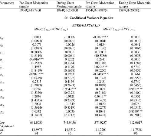
a VAR(2)-BEKK for both sets in the second subsample. Table 3 reports the estimated
conditional variances with associated log-likelihood and SIC values, and numbers of
observations.
[Table 3 HERE]
The results of the first part of Table 3 (the conditional mean equations)indicate that the growth
rates of home mortgages and output are affected only by their own lagged values, in both
1954Q3-1978Q4 and 1984Q1-2008Q1. The insignificance of the cross terms ( 12, 21, 12, 21)
suggests that there is no interaction between the two variables, and therefore no spillovers in
means. Growth rates of home mortgages and of residential investment are both influenced by
their own lagged terms, and by lagged values of the other variable. This interaction, and thus the
13 Now consider the conditional variance results in the second part of Table 3. Coefficients 12
and 21 are indirect effects (spillover effect) while g12 and g21 are direct effects. For instance,
coefficient a12 indicates if innovations in mortgage growth in quarter t decreases the conditional
variance of output growth in quarter t+1. The estimation results do not support this, but we do observe volatility spillovers from output growth to home mortgage growth in the first subsample
(coefficient value 21 = -0.2071). We also detect volatility spillovers in both directions between
home mortgage growth and residential investment growth (7.04% and -4.84% respectively). In
contrast, during the Great Moderation none of these volatility spillovers can be detected.
Moreover, we detect that before the Great Moderation an increase in the volatility of mortgage
growth causes an increase in the volatility of output growth (coefficient value g12=0.0911). In order to test causality in variance (the purpose for which we did the estimations) we need
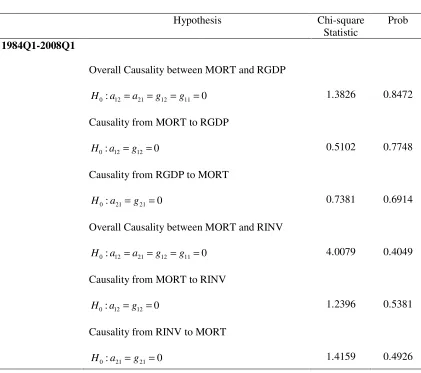
to consider both the indirect and direct effects and compute test statistics. Table 4 reports the test
results.
[Table 4 HERE]
Before the Great Moderation, we observe overall causality in variance between home mortgages
growth and output growth, based on unidirectional causality from output growth volatility to the
volatility of home mortgages growth. In terms of variances, mortgage finance was driven by
real-sector fundamentals during 1954Q3-1978Q4. Second, we detect overall causality in variance
between home mortgages growth and growth of residential investment, based on their
bidirectional causality. Variances of mortgages and residential investment growth rates moved
together during 1954Q3-1978Q4. Both these findings are absent in the second subsample.
This is in line with the CDGM hypothesis, which attributes lower output volatility to the
partial decoupling of finance from the real sector and of the (volatility of) mortgages from its
primary use in supporting residential investment. These conditions would facilitate a trend in
which mortgage (and other) finance came to support consumption growth that was
countercyclical to GDP shocks (Table 1), so lowering the volatility of GDP. Thus, these findings
are supportive of the CDGM hypothesis.
Finally, we study residual diagnostics for the VAR-unrestricted BEKK models in order to
14 standardized residuals for two lag lengths (8 and 12 quarters) is not statistically significant (p =
0.01) except in the first subsample for the growth rate of home mortgages, which exhibits
remaining autocorrelation. We also compute squared standardized residuals and compute the
Q-statistic, which is never significant (p=0.01). Hence we cannot reject the null hypothesis of no
remaining ARCH effects along the two lag lengths in both subsamples.
[Table 5 HERE]
5. Summary, Discussion and Conclusions
Financial innovation during the Great Moderation increased credit flows both in volume and
with regard to the range of activities and investments they could finance. We hypothesize that a
larger part of economic activity was debt-financed during the Great Moderation than before, and
that those debt-financed incomes moved more independently from other GDP components,
leading to a reduction in overall output volatility. We refer to this hypothesis as the ‘credit-driven
Great Moderation hypothesis’ (or CDGM hypothesis, for short).
Specifically, we hypothesize that during the Great Moderation (i) growth in mortgage
finance partly decoupled from fundamentals as measured by overall output growth and (ii) this
allowed mortgage finance less to finance residential investment and by implication, more to
finance spending on other GDP components. We document that the start of the Moderation
coincided with a surge in bank credit creation (especially mortgage credit), a rise in property
income, a rise in the consumption share of GDP, and a change in correlation (from positive to
negative) between consumption and non-consumption GDP components (investment, export and
government expenditure).
We test the CDGM hypothesis formally by studying causality-in-variance of home mortgage
lending, residential investment and total output, in a multivariate GARCH framework for the
U.S. both over two periods, 1954-1978 (before the Great Moderation) and 1984-2008 (during the
Great Moderation). It is significant that we test in variances rather than levels since the Great
15 also of the financial-sector variables that possibly caused it (Bean, 2011). Testing in variances
allows for potential interaction of volatilities, which are not captured in the literature to date.
We estimate a bivariate unrestricted BEKK model and conduct causality-in-variance tests
following Caporale et al. (2002). We observe unidirectional causality in variance from total
output to mortgage lending before the Great Moderation, which is no longer detectable during
the Great Moderation. We also find that bidirectional causality in variance of home mortgage
lending and residential investment existed before, but not during the Great Moderation. Both
these findings are consistent with a credit-driven Great Moderation view, in conjunction with
other explanations. We conclude with a discussion of its place in the wider literature and
suggestions for future research.
The present paper presents the argument that the Great Moderation was (partly) caused by a
surge and shift in credit flows. It so provides a basis to connect the Great Moderation to the
‘Great Panic’ and the ‘Great Depression’ as in Bean (2011). Empirically, Kemme and Roy
(2012) utilize vector error correction models and panel probit and logit models to show that the
U.S. mortgage-driven house price boom was a good predictor of the current crisis. The present
paper also provides a link between Moderation and Crash: perhaps there was a moderation of
volatility partlydue to immoderate credit growth.
The paper is consistent with, but different in focus from, other papers that take a ‘financial
sector view’ of the Great Moderation. Increased liquidity is a common outcome of financial
innovations (Blanchard and Simon, 2001, Dynan et al., 2005), financial sector development
(Easterly et al., 2000) and improvements in monetary policy (Clarida et al., 2000; Bernanke,
2004). The novel contribution of this paper is that it attempts to analyse how this increase
combined with a shift in the relation of credit aggregates (mortgage lending) with fundamentals
(output growth) on the one hand, and with the financing of output components (residential
investment) on the other hand. Methodologically, this paper presents a case for testing these
relations in variance, since the Great Moderation is a puzzle about second moments (as also
Bean, 2011 stresses). This is a major reason for our different findings from the closely related
paper by Den Haan and Sterk (2010). In the present perspective, it is too early to write of ‘the
myth of financial innovation and the Great Moderation’ (Den Haan and Sterk, 2010:707).
In pursuing additional evidence or falsification of the CDGM hypothesis, several lines of
16 countercyclical GDP components. The Table 1 correlations suggests that much of this is
consumption in one form or another. But as noted, there is no simple link from changes in the
use of mortgage finance to growth in a defined statistical category such as ‘durable goods
consumption’. Also, including total consumption (the larger part of GDP) in the model poses
serious endogeneity problems13. Whatever the precise delineation however, the channel through
which mortgage growth feeds into growth of consumption (or other spending categories) is
plausibly home equity withdrawal. Finding better, and especially longer, time series for home
equity withdrawal than are presently available (Greenspan and Kennedy, 2008) is a major
challenge, but potentially fruitful.
Second, home mortgages are one instance (though the most important one) of credit flows
that supported the price boom in all kinds of assets within the ‘Finance, Insurance and Real
Estate’ category of the U.S. National Income and Product Accounts. Another way therefore of
pursuing the CDGM hypothesis is to aggregate all these financial-sector credit flows rather than
focusing on one of them. Any credit flows supporting the realization of capital gains which could
then be used to smooth consumption is in principle relevant to the CDGM hypothesis. This
would include bank credit supporting mortgage products but also those of pension funds, savings
institutions, credit unions, funding corporations, exchange traded funds, money market mutual
funds, and the like. There is broad agreement on the wealth effects of capital gains in these assets
(through e.g. equity withdrawal, asset sales and share buybacks) but no research has been
undertaken on the consequences for output volatility during the Great Moderation. Widening the
definition of assets on which wealth effects operate might just introduce noise in the analysis (if
house wealth really were the major or only relevant asset class), or it might provide a more
complete view of wealth effects on output volatility during the Great Moderation. Exploring this
is a fruitful avenue for future research.
13
17
[image:18.595.68.486.220.500.2]TABLES
Table 1: Trends in Credit and the Macroeconomy Before and During the U.S.
Great Moderation
(decade averages) 1970s 1980s 1990s 2000s*
Consumption** (% GDP)
62.4 64.3 67.0 69.9
correlation of consumption growth with non-consumption growth (coefficient)**
25.4 -35.8 -35.8 -40.4
total US domestic bank credit stock *** (% GDP)
147.3 186.1 236.7 297.0
bank mortgage credit stock (% GDP)
14.5 29.1 54.9 96.3
Income from property (% GDP)
30.0 41.7 40.5 38.9
Volatility of GDP growth (annual s.d., '000)
10.5 11.4 5.4 6.3
Source: Bureau of Economic Analysis
Note: all decadal figures are unweighted averages calculated from nominal quarterly data. * The 2000s include the 8 years of 2000 to 2007.
** The ‘non-consumption’ part of GDP comprises investment, export and government expenditures; the ‘consumption’ part includes private consumption. ‘Correlation’ is a two-year moving average of correlations between quarterly observations of differenced growth rates.
18
Table 2: Descriptive Statistics
Mean Std dev. Skewness Kurtosis LM-Statistic JB
1954Q3-1978Q4
MORT 0.0235 0.0091 0.0887 4.6216 19.8769* (12)
10.7556
RGDP 0.0094 0.0109 -0.3512 3.5788 33.1762*** (12)
3.3477
RINV 0.0088 0.0501 -0.1068 3.2299 4.8668* (2)
0.3981
1984Q1-2008Q1
MORT 0.0232 0.0092 0.3121 2.4492 40.1714*** (12)
2.7721
RGDP 0.0074 0.005 -0.2454 3.2731 3.5213* (1)
1.2620
RINV 0.0029 0.0284 -0.8581 3.5416 10.3171* (5)
12.9547
19
Table 3: VAR-BEKK (unrestricted) Estimates
Parameters Pre-Great Moderation sample During-Great Moderation sample Pre-Great Moderation sample During-Great Moderation sample
1954Q3-1978Q4 1984Q1-2008Q1 1954Q3-1978Q4 1984Q1-2008Q1
(a) Conditional Mean Equation
VAR(1) VAR(2) VAR(1) VAR(2)
MORT (y1t)-RGDP (y2t) MORT (y1t)-RINV (y2t)
1 µ 0.0039*** (0.0013) 0.0051* (0.0027) 0.0037** (0.0014) 0.0039** (0.0019) 2 µ 0.0074** (0.0037) 0.0044** (0.0022) 0.0343** (0.0150) 0.0064 (0.0072)
(
)
11 y1 1t
γ − 0.8337***
(0.0530) 0.4878*** (0.1040) 0.8386*** (0.0573) 0.4429*** (0.0938)
(
)
12 y2t1
γ − 0.0042
(0.0448) -0.1282 (0.1109) 0.0272*** (0.0094) -0.0147 (0.0310)
(
)
21 y1 1t
γ − 0.0165
(0.1417) 0.0368 (0.0916) -1.1905* (0.6309) 0.1495 (0.3199)
(
)
22 y2t1
γ − 0.2434**
(0.1025) 0.10159 (0.1226) 0.4514*** (0.1047) 0.6611*** (0.1342)
(
)
11 y1t 2
θ − 0.3408***
(0.1057)
0.3863*** (0.1009)
(
)
12 y2t 2
θ − -0.0468
(0.1500)
0.0452 (0.0348)
(
)
21 y1t 2
θ − -0.0260
(0.0728)
-0.3433 (0.3532)
(
)
22 y2t 2
θ − 0.3048**
(0.1228)
20
Table 3 (continued)
Parameters Pre-Great Moderation sample During-Great Moderation sample Pre-Great Moderation sample During-Great Moderation sample
1954Q3-1978Q4 1984Q1-2008Q1 1954Q3-1978Q4 1984Q1-2008Q1
(b) Conditional Variance Equation
BEKK-GARCH(1,1)
MORT (y )-RGDP (1t y ) 2t MORT (y )-RINV (1t y ) 2t
11 c 0.0013 (0.0093) -0.0006 (0.0021) -0.0028*** (0.0004) 0.0010 (0.0010) 12 c -0.0074 (0.0887) -0.0026 (0.0071) -0.0134 (0.0126) 0.0041 (0.0063) 22 c 0.00006 (9.8149) 0.0031 (0.0061) 0.00001 (40.3586) 0.0030 (0.0053) 11 a -0.5916*** (0.1552) 0.1202 (0.1384) -0.2941 (0.2101) 0.0010 (0.1787) 12
a 0.4937
(0.8419) 0.1170 (0.1638) 0.0704*** (0.0250) 0.5740 (0.5456) 21 a -0.2071*** (0.0419) 0.1963 (0.2727) -0.0484*** (0.0141) 0.0661 (0.0556) 22
a -0.2313
(0.2073) 0.4139 (0.2673) -0.2431 (0.1898) 0.5740 (0.5456) 11 g 0.0216 (0.5320) 0.9642*** (0.0372) 0.0021 (0.2189) 0.9682*** (0.0400) 12
g 0.2936
(1.4335) -0.0421 (0.2329) 0.0911** (0.0427) 0.0352 (0.2316) 21
g 0.2008
(0.5614) -0.1249 (0.8319) -0.0122 (0.0277) -0.0281 (0.0317) 22 g 0.6332 (1.1407) -0.0036 (2.1717) 0.1041 (0.4478) 0.8639*** (0.0906) Log Likelihood
691.8080 744.9436 574.0287 612.0617
SIC -13.8977 -14.5212 -11.2700 -11.7528
N 94 96 95 96
[image:21.595.55.554.140.592.2]21
Table 4: Granger Causality Tests in Variance
Hypothesis Chi-square
Statistic
Prob
1954Q3-1978Q4
Overall Causality between MORT and RGDP
0: 12 21 12 11 0
H a =a =g =g = 25.1290 0.0000
Causality from MORT to RGDP
0: 12 12 0
H a =g = 0.3457 0.8413
Causality from RGDP to MORT
0: 21 21 0
H a =g = 24.5918 0.0000
Overall Causality between MORT and RINV
0: 12 21 12 11 0
H a =a =g =g = 6.02901 0.0000
Causality from MORT to RINV
0: 12 12 0
H a =g = 9.9533 0.0069
Causality from RINV to MORT
0: 21 21 0
22
Table 4 (continued)
Hypothesis Chi-square
Statistic
Prob
1984Q1-2008Q1
Overall Causality between MORT and RGDP
0: 12 21 12 11 0
H a =a =g =g = 1.3826 0.8472
Causality from MORT to RGDP
0: 12 12 0
H a =g = 0.5102 0.7748
Causality from RGDP to MORT
0: 21 21 0
H a =g = 0.7381 0.6914
Overall Causality between MORT and RINV
0: 12 21 12 11 0
H a =a =g =g = 4.0079 0.4049
Causality from MORT to RINV
0: 12 12 0
H a =g = 1.2396 0.5381
Causality from RINV to MORT
0: 21 21 0
[image:23.595.74.495.126.499.2]23
Table 5: Residual diagnostics
MORT,t
ε εRGDP,t εRINV,t
1954Q3-1978Q4
Q(8) 24.613
[0.002]
3.6047 [0.891]
7.6552 [0.468]
Q2(8) 3.5104
[0.898]
2.1571 [0.976]
13.574 [0.094]
Q(12) 40.252
[0.000]
8.305 [0.761]
10.669 [0.557]
Q2(12) 6.3648
[0.897] 4.8547 [0.963] 18.320 [0.106] 1984Q1-2008Q1
Q(8) 15.903
[0.044]
5.4035 [0.714]
9.7428 [0.284]
Q2(8) 6.2651
[0.618]
8.1651 [0.418]
14.541 [0.069]
Q(12) 19.324
[0.081]
13.684 [0.321]
13.923 [0.306]
Q2(12) 12.662
[0.394]
12.479 [0.408]
14.994 [0.242]
24
References
Acemoglou, D. and F. Zilibotti (1997), “Was Prometheus Unbound by Chance? Risk,
Diversification, and Growth,” Journal of Political Economy 105: 709-51.
Acemoglou, D., S. Johnson, J. Robinson and Y. Thaicharoen (2003), “Institutional Causes,
Macroeconomic Symptoms: Volatility, Crises and Growth,” Journal of Monetary Economics
50: 49-123.
Ahmed, S., A. Levin and B. Wilson (2002), “Recent U.S. Macroeconomic Stability: Good Luck,
Good Policies, or Good Practices?,” International Finance Discussion Papers 730, Board of Governors of the Federal Reserve System (U.S.).
Alaganar, V. and R. Bhar (2003), “An International Study of Causality-in-Variance: Interest Rate
and Financial Sector Returns,” Journal of Economics and Finance 27: 39-55.
Barnett, W. and M. Chauvet (forthcoming), “The End of the Great Moderation? How Better
Monetary Statistics Could Have Signaled the Systemic Risk Precipitating the Financial
Crisis,” Journal of Econometrics Annals.
Bauwens, L., S. Laurent and J. Rombouts (2006), “Multivariate GARCH Models: A Survey,”
Journal of Applied Econometrics 21: 79-109.
Bean, C. (2011), “Joseph Schumpeter Lecture: The Great Moderation, the Great Panic, and the
Great Contraction,” Journal of the European Economic Association 8: 289-325.
Benati, L. and P. Surico (2009), “VAR Analysis and the Great Moderation,” American Economic Review 99: 1636-52.
Benk, S., M. Gillman and M. Kejak (2005), “Credit Shocks in the Financial Deregulatory Era:
25 Bernanke, B. (1993), “Credit in the Macroeconomy,” Quarterly Review, Federal Reserve Bank
of New York issue Spr: 50-70.
Bernanke, B. (2004), “The Great Moderation,” Speech at the meetings of the Eastern Economic Association, Washington, D.C., February 20.
Bernanke, B. and M. Gertler (1995), “Inside the Black Box: The Credit Channel of Monetary
Policy Transmission,” Journal of Economic Perspectives 9: 27-48.
Blanchard, O. and J. Simon (2001), “The Long and Large Decline in U.S. Output Volatility,”
Brookings Papers on Economic Activity 1: 135-74.
Bliss, R. and G. Kaufmann (2003), “Bank Procyclicality, Credit Crunches, and Asymmetric
Policy Effects: A Unifying Model,” Journal of Applied Finance 13: 23-31.
Boivin, J., and M. Giannoni (2006), “Has Monetary Policy Become More Effective?,” The Review of Economics and Statistics 88: 445-62.
Bollerslev, T, R Engle and J Wooldridge (1988), “A Capital Asset Pricing Model with Time
Varying Covariances,” Journal of Political Economy 96: 116-31.
Bollerslev, T. (1986), “Generalized Autoregressive Conditional Heteroskedasticity,” Journal of Econometrics 31: 307-27.
Bollerslev, T. (1990), “Modelling the Coherence in Short-Run Nominal Exchange Rates: A
Multivariate Generalized Arch Model,” The Review of Economics and Statistics 72: 498-505.
26 Campbell, S. (2005), “Stock Market Volatility and the Great Moderation,” FEDS WP, 2005-47,
Board of Governors of the Federal Reserve System.
Canning, D., L.A.N. Amaral, Y. Lee, M. Meyer and H.E. Stanley (1998), “Scaling the Volatility
of the GDP Growth Rate,” Economics Letters 60: 335-41.
Caporale, G. and P. Howells (2001), “Money, Credit and Spending: Drawing Causal Inferences,”
Scottish Journal of Economics 48: 547-57.
Caporale, G., N. Pittis and N. Spagnolo (2002), “Testing for Causality-in-Variance: An
Application to the East Asian Markets,” International Journal of Finance and Economics 7: 235-45.
Carroll, C., M. Otsuka and J. Slacalek (2006), “How Large Is the Housing Wealth Effect? A
New Approach,” NBER Working Paper No. 12746.
Cechetti, A. and S. Krause (2006), “Assessing the Sources of Changes in Volatility of Real
Growth,” NBER Working Paper No. 11946.
Cheung, Y. and L. Ng (1996), “A Causality-in-Variance Test and its Application to Financial
Market Prices,” Journal of Econometrics 72: 33-48.
Clarida, R., J. Gali, and M. Gertler (2000), “Monetary Policy Rules and Macroeconomic
Stability: Evidence and Some Theory,” The Quarterly Journal of Economics 115: 147-80.
Cogley, T. and T. Sargent (2005), “Drifts and Volatilities: Monetary Policy and Outcomes in
the Post-WWII US”, Review of Economic Dynamics 8: 262-302.
Davis S. and J. Kahn (2008), “Interpreting the Great Moderation: Changes in the Volatility of
27 Den Haan, W. and V. Sterk (2010), “The Myth of Financial Innovation and the Great
Moderation,” The Economic Journal 121: 707-39.
Dickey, D. and W. Fuller (1979), “Distribution of the Estimators of Autoregressive Time Series
with a Unit Root,” Journal of the American Statistical Association 74: 427-31.
Dijk, D. van, D. Osborn and M. Sensier (2005), “Testing for Causality in Variance in the
Presence of Breaks,” Economics Letters 89: 193-99.
Dynan, K., D. Elmendorf and D. Sichel (2006), “Can Financial Innovation Help to Explain the
Reduced Volatility of Economic Activity?,” Journal of Monetary Economics 53: 123-50.
Easterly, W., M. Kremer, L. Pritchett and L. Summers (1993), “Good Policy or Good Luck?
Country Growth Performance and Temporary Shocks,” Journal Of Monetary Economics
32:459-83.
Easterly, W., R. Islam and J. Stiglitz (2000), “Shaken and Stirred: Explaining Growth
Volatility,” Paper at the 2000 Annual World Bank Conference on Development Economics.
Engle, R. (1982), “Autoregressive Conditional Heteroskedasticity with Estimates of the Variance
of United Kingdom Inflation,” Econometrica 50: 987-1007.
Engle, R. (2002), “Dynamic Conditional Correlation-A Simple Class of Multivariate GARCH
Models,” Journal of Business and Economic Statistics 20: 339-50.
Engle, R. and K. Kroner (1995), “Multivariate Simultaneous Generalized ARCH,” Econometric Theory 11: 122-50.
Fang, W. and S. Miller (2008), “The Great Moderation and the Relationship between Output
28 Fogli, A. and F. Perri (2006), “The "Great Moderation" and the US External Imbalance,” NBER
Working Paper No. 12708.
Gambetti, L., E. Pappa, and F. Canova (2008), “The Structural Dynamics of US Output and
Inflation: What Explains the Changes?,” Journal of Money, Credit, and Banking 40: 369–88.
Glymour, C. and G. Cooper (1999), Computation, Causation, and Discovery, The MIT Press, Cambridge, MA, USA.
Greenspan A. and J. Kennedy (2008), “Sources and Uses of Equity Extracted from Homes.”
Oxford Review of Economic Policy 24: 120-44.
Guerron-Quintana, P. (2009), “Money Demand Heterogeneity and the Great Moderation,”
Journal of Monetary Economics 56: 255-66.
Hafner, C. and H. Herwartz (2004), “Testing for Causality in Variance Using Multivariate
GARCH Models,” Working Paper No. 03.
Hamilton, J. (2008), “Macroeconomics and ARCH,” NBER Working Paper No. 14151.
Hong, Y (2003), “Extreme Risk Spillover between Chinese Stock Markets and International
Stock Markets,” Working Paper.
Hong, Y. (2001), “A Test for Volatility Spillover with Application to Exchange Rates,” Journal of Econometrics 103: 183-224.
Jaimovich, N. and H. Siu (2009), “The Young, the Old, and the Restless: Demographics and
29 Kahn, J., M. McConnell and G. Perez-Quiros (2002), “On the causes of the increased stability of
the U.S. economy,” Federal Reserve Bank of New York Economic Policy Review 8: 183-202.
Kanas, A. and G. Kouretas (2002), “Mean and Variance Causality between Official and Parallel
Currency Markets: Evidence form Four Latin American Countries,” The Financial Review
37: 137-64.
Kemme, D. and S. Roy (2012), “Did the Recent Housing Boom Signal the Global Financial
Crisis?,” Southern Economic Journal 78: 999-1018.
Kim, C. and C. Nelson (1999), “Has the U.S. Become More Stable? A Bayesian Approach Based
on a Markov-Switching Model of the Business Cycle,” Review of Economics and Statistics
81: 08-16.
Kiyotaki, N. and J. Moore (1997), “Credit Cycles,” Journal of Political Economy 105: 211-48.
Kocherlakota, N. (2000), “Creating Business Cycles Through Credit Constraints,” Federal Reserve Bank of Minneapolis Quarterly Review 24: 2-10.
Kwiatkowski, D., P Phillips, P. Schmidt and Y. Shin (1992), “Testing the Null Hypothesis of
Stationarity Against the Alternative of a Unit Root,” Journal of Econometrics 53: 159-78.
Laurent, S. and J-P Peters (2002), “G@RCH 2.2: An OX Package for Estimating and
Forecasting Various ARCH Models,” Journal of Economic Surveys 16: 447-85.
Li, G., J. Refalo and L. Wu (2008), “Causality-in-Variance and Causality-in-Mean among
European Government Bond Markets,” Applied Financial Economics 18: 1709-20.
30 Lown C. and D. Morgan (2006), “The Credit Cycle and the Business Cycle: New Findings Using
the Loan Officer Opinion Survey,” Journal of Money, Credit, and Banking 38: 1575-97.
Lubik, T., and F. Schorfheide (2003), “Computing Sunspot Equilibria in Linear Rational
Expectations Models,” Journal of Economic Dynamics and Control 28: 273-85.
McCarthy, J. and E. Zakrajsek (2007), “Inventory Dynamics and Business Cycles: What Has
Changed?,” Journal of Money, Credit and Banking 39: 591-613.
McConnell, M. and G. Perez-Quiros (2000), “Output Fluctuations in the United States: What
Has Changed since the Early 1980’s,” American Economic Review 90: 1464-76.
Mendicino, A. (2007), “Credit Market and Macroeconomic Volatility,” European Central Bank Working Paper Series No. 743.
Nakov, A. and A. Pescatori (2010), “Oil and the Great Moderation,” The Economic Journal 120: 131-56.
Owyang, M.T., J. Piger and H. Wall (2007), “A State-Level Analysis of the Great Moderation,”
Federal Reserve Bank of St Louis, Working Paper No. 003B.
Pantelidis, T. and N. Pittis (2004), “Testing for Granger Causality in Variance in the Presence of
Causality in Mean,” Economics Letters 85: 201-7.
Phillips, P. and P. Perron (1988), “Testing for a Unit Root in Time Series Regression,”
Biometrika Trust 75: 335-46.
Primiceri, G. (2005), “Time Varying Structural Vector Autoregressions and Monetary Policy,”
31 Sims, C. and T. Zha (2006), “Were There Regime Switches in U.S. Monetary policy?,”
American Economic Review 96: 54-81.
Spirtes, P., C. Glymour and R. Scheines (2000), Causation, Prediction and Search, The MIT Press, Cambridge, MA, USA.
Stock, J. and M. Watson, “Has the Business Cycle Changed and Why?,” National Bureau of Economic Research, Inc., working paper 9127 (2002).
Summers, P. (2005), “What Caused the Great Moderation? Some Cross-Country Evidence,”
Federal Reserve Bank of Kansas City Economic Review, 3rd Quarter.
Tse, Y. and A. Tsui (2002), “A Multivariate GARCH Model with Time-Varying Correlations,”
Journal of Business and Economic Statistics 20: 351-62.
Uhlig, H. (2004), “What Moves GNP?,” Econometric Society 2004 North American Winter Meetings 636.
Warnock, M. and F. Warnock (2000), “The Declining Volatility of U.S. Employment: Was