Pakistan Economy DSGE Model with Informality

Munich Personal RePEc Archive

Pakistan Economy DSGE Model with

Informality

Ahmed, Shahzad and Ahmed, Waqas and Khan, Sajawal and

Pasha, Farooq and Rehman, Muhammad

State Bank of Pakistan, Research Department

April 2012

1 Introduction

Dynamic Stochastic General Equilibrium (DSGE) models have become a work-horse for policy makers and central bankers for comparing possible impact of di¤erent policy scenarios. The proponents of these models claim that DSGE models are capable of replicating a number of stylized business cycle facts, for di¤erent developed and emerging economies, and are also not subject to the Lucas Critique [Pichler, (2007)]. In the last two decades signi…cant progress has been made regarding speci…cation and estimation of these models according to the need and features of the economy at hand. The most important recent contributions in terms of speci…cation and standardization of modeling proce-dures involved in DSGE modeling are due to Smets and Wouters (2003) and Christiano, et al. (2005). As a result of this signi…cant improvement in DSGE modeling literature many central banks of advanced countries have already developed their DSGE models recognizing the usefulness of these models for policy analysis and forecasting. Following the example of developed countries many of the emerging economies are also now focusing on constructing DSGE models for their countries encompassing relevant features of their respective economies.

The original DSGE models are actually the extension of real business cycle (RBC) models. Kydland and Prescott (1982) laid the foundation of DSGE modeling in the spirit of RBC theory. Real Business Cycle theory, assuming price ‡exibility and rationality of optimizing agents facing some constraints, investigates quarterly ‡uctuations when economy is hit by a real shock (the most common one being a technology shock). The earlier RBC models were criticized because economic policies had no role to play in these models. Fur-thermore these models failed to replicate some of the empirical regularities such as liquidity e¤ects, co-movement of productivity and employment or the co-movement of real wages and output (Kremer et al., 2006). However, over time, there has been extensive work done that has helped in making these models theoretically parsimonious and empirically sound.

as-sumptions were introduced into DSGE models. For example, …nancial sector rigidities (Christensen and Dib, 2008), asymmetric information (Collard and Dellas, 2004), habit persistence in consumption (Fuhrer, 2000), adjustment costs in investment and variable capital utilization (Smets and Wouters, 2003 and 2005), and customer hold-up e¤ects (Aksoy et al., 2009).

These models have been reasonably successful in replicating business cycles features of developed economies and have gained considerable importance for policy analysis and forecasting at central banks around the western world. However, for developing countries like Pakistan the adoption of such models requires a signi…cant amount of groundwork and customization i.e. to be con-sistent with relevant micro evidence. However, any information about even the basic micro foundations of Pakistan economy is di¢cult to obtain as there is an inherent lack of micro-based surveys and even appropriate frequency data of major macroeconomic variables is mostly unavailable. Furthermore the lack of forward looking variables available in developing countries further compli-cates the situation. These challenges related to unavailability and consistency of micro-macro data tend to be understated when it comes to developing DSGE models for developing countries. For most of the existing literature on DSGE models for emerging economies, key parameters are borrowed from the literature and data transformation remains inadequate. One major contribu-tion of this paper is that it overcomes some of these issues to a certain extent. This has been done through conducting wage and price setting surveys of manufacturing …rms both in the formal and infomal sectors representing all the subsectors under manucturing in Pakistan. Besides, we have tried to use respresntative micro level datasets made available by Federal Bureau of Statis-tics (e.g., Labor Force Survey) and compiled e¤ectively by us at the Research Department.

In addition, certain features of an economy like Pakistan cannot be anchored on the results of similar features from the developed world due to distinctly di¤erent developing nature of emerging economies. So the blueprint of mod-els borrowed from advanced economies would not work for these economies without bringing them in line with relevant economic structure prevailing in a given economy. Some of the common features of emerging economies which di¤erentiate them from developed economies need to be embedded in the eco-nomic models for meaningful policy implications include:

i) Existence of a large informal sector;

ii) Small open economies vulnerable to external shocks;

iii) Weak …nancial sector;

Keeping in view the signi…cance of above issues, the objective of this project is to develop a preliminary DSGE model of Pakistani economy consistent with some of the key economic features of Pakistan. Since this is the very …rst attempt to do so we are prioritizing the inclusion of only one feature in the otherwise standard DSGE model on the basis of our subjective degree of pref-erence. As a result we incorporate informality in labor and product markets in a simple DSGE model. Future versions of the model would incorporate other relevant economic features of Pakistan.

2 Modeling with Informality: Literature on Developing Economies

Most of the literature on DSGE models has attempted to explain business cycle ‡uctuations of advanced economies with well established business cy-cles features, but literature on business cycy-cles of emerging economies is very limited. However, in the past few years some e¤orts have been made in devel-oping DSGE models capable of capturing the business cycle ‡uctuations for emerging economies. DSGE modeling for developing countries poses a number of challenges where not only the economic environment is di¤erent but is also less well-known. To exacerbate the situation further important features (even the stylized facts) of such economies are also not well established.

Batini et al. (2011) has recently developed a DSGE model for Indian economy with informality in goods market in the presence of credit constraints. They also introduced labor market frictions in the formal sector a la Zenou (2008). They used Bayesian technique for estimating parameters and have shown that the inclusion of informal sector and …nancial frictions improved the …t of their model. Peiris and Saxegaard (2007) introduced credit frictions in the presence of informality with an assumption that part of the inputs used in the production process are …nanced through borrowing at a premium over deposits from the informal sector. The study was aimed at evaluating monetary policy trade-o¤s in low-income countries with informal lending sources. The model was estimated using data for Mozambique.

Conesa et al. (2002) incorporated informal goods producing sector with dif-ferentiated technology in a simple RBC model. In this model sector trade-o¤ is allowed through the presence of a wage premium in the formal sector. Fur-thermore, labor is assumed to be indivisible in the formal sector. Households can choose working between the two sectors with a given probability. A worker in the informal sector can enjoy more leisure but at the cost of lower wage.

money, in terms of an in‡ation tax, on the informal sector. They tried to show the e¤ect of the informal sector on optimal policy choice by government.

Aruoba (2010) and Aruoba and Schorfheide (2011) also introduced cash-in-advance constraint to di¤erentiate informal sector from the formal sector by assuming that money is the only medium of exchange used in the informal sector. In their paper, using a very speci…c search-based monetary model, they found that large informal sector gets smaller in size and overall tax collection becomes higher under rising in‡ation.

Mattesini and Rossi (2010) analyzed the monetary policy in a dual economy in the New Keynesian framework with one competitive (informal) and one unionized (formal) sector. They came up with the conclusion that level of output is associated with relative size of the two sectors.

Castillo and Montoro (2008) modeled their economy with frictions in the labor market by introducing formal and informal labor contracts and analyzed the interaction between the two sectors and monetary policy. They introduced informality through hiring costs owing to labor market conditions (degree of tightness). In their model …rms in the wholesale sector are assumed to balance the high productivity in formal sector with the lower hiring costs faced by the informal sector. The main …nding of this theoretical framework is the cyclical behavior of informal sector i.e. it expands with rising aggregate demand because of lower hiring costs. Through this channel a link between informality, the in‡ation dynamics and monetary policy is established. This study supports the idea of informal labor market being a bu¤er for an economy.

Our model is closest to Conesa et al. (2002) in the sense that we introduce an informal goods producing sector with di¤erentiated technology, as well as informality in labor market in a simple RBC model. However, we di¤erentiate formal and informal sectors’ labor on the basis of skill from the same household rather than assuming that households can choose between working for the two sectors with a given probability. In this way we have segmented the labor market with ‡exibility that households can decide on working hours of labor supplied to each of the two sectors, formal and informal, which maximizes overall utility of the households. A wage premium is charged in the formal sector over wage in the informal sector due to monopoly of households on skilled labor.

informal sector as well (various Labor Force Surveys, FBS).

Furthermore, the frequency of our model is annual making a stronger case for RBC type model. This is further supported by …nding that annual price rigidity does not hold for Pakistan. Choudhary et al. (2011) …nd that all the …rms in their sample of Pakistani formal …rms adjust prices within a year irrespective of the competition they face. They also show that at least in the manufacturing sector 58 percent …rms are connected with the informal sector either through demand or supply channels where demand channels tend to dominate. This motivated us to model the production of goods and services in the informal sector along with the formal sector.

3 Model

The model incorporates the informal sector through production as informal-ity is one of the striking features of the developing countries. In our model, economy consists of households, …rms, government and a monetary authority. There are two types of …rms; formal and informal. These …rms are further classi…ed as intermediate and …nal good producing …rms. Intermediate good producing …rms sell their products to the …nal good producer, where the …nal good producing …rms are only the retailers. Households derive utility from leisure, real money balances and consumption. They also supply labor and rent capital to …rms. Each household has a unit of labor which is a composite of formal (skilled) and informal (unskilled) labor. The formal (skilled) labor is further divided into di¤erent types. Households have monopoly over each type "r" of labor which gives them the market power in wage setting process of such types of formal labor.

The …nal goods are produced by using intermediate goods. Di¤erentiated goods produced by the formal intermediate …rms, employing hired labor and capital, are sold to formal …nal good producers in a monopolistically com-petitive market. Labor is the only input used in the production of informal intermediate goods, which are sold to informal …nal good producers in a per-fectly competitive market, which we assume for simpli…cation.

government spending shock/…scal shock; and an interest rate shock.

3.1 The Household

The representative household’s utility function consists of consumption, ct,

real money balances,Mt

Pt, and leisure 1 ht . The total time endowment to the

household is normalized to one. The preferences of the representative house-hold can be described by the following life time expected utility function:

U(:) = Et

X _t

Ut(ct;

Mt

Pt

;1 ht) (1)

wherehtis total number of hours worked and (0;1)is the discount factor.

This particular utility function is also called the money in the utility function (MIU). The main reason for adopting this particular functional form for utility is the size of the informal sector in Pakistan which is essentially based on cash transactions as in Arby et al. (2010). Therefore, preference for holding more cash is a reasonable assumption for our economy.

U(:) = lnc(i) + lnM(i)

P

h(i)1+

1 + (2)

where is the preference parameter on money holding. Here we would like to make it a point to note that upper-case letters would denote nominal vari-ables and lower-case letter denote real varivari-ables. The household faces following budget constraint while making its decisions:

ct+it+

Mt

Pt

+ Bt

Pt

= Wt

Pt

ht+

Rk t

Pt

kt+

Mt 1

Pt

+ (1 +Rt 1)

Bt 1

Pt

+ Tt

Pt

+ t

Pt

(3)

The left hand side of (3) represents household’s total expenditures, while its right hand side represents its total earnings whereit, Bt, Wt, Rkt, kt, Rt,Tt ,

and represent investment, bond holdings, nominal wage rate, rent on capital, capital, interest rate on bonds, lump- sum transfers, and dividends/pro…t from …rms respectively. Capital gets accumulated according to:

kt+1 = (1 )kt+it (4)

where (0;1)is the capital depreciation rate. Household choosesct,Mt,Bt,

ht, andkt, given (3) and (4), so that its life time expected utility is maximized.

First order conditions of the household’s utility maximization problem are given as:

1

ct

= (1 +Rt)Et

1

t+1ct+1

Et

"

t+1

(1 +Rt)

n

(1 ) +rk

t+1 o#

= 1 (6)

ht=

wt

ct

1

(7)

and

Mt=Pt

= 1

ct

Et

1

t+1ct+1

(8)

where (5) is the typical Euler equation for consumption, (7) is the labor supply equation and money demand is given by (8). (6) equates real rate of return on bonds and capital.

3.1.1 Labor Supply Choice between Formal and Informal Sectors

Household’s aggregate labor is a composite of both formal, hF

t, and informal

labour, hI

t. It can be expressed as:

ht= # hFt

1+#

+ (1 ) # hIt

1+# 1+1#

(9)

where fractions and (1 ) represent formal and informal labor division of the representative household respectively. Similarly the aggregate wage can be expressed as:

Wt = WtF

#

1+#

+ (1 ) WtI

#

1+#

1+# #

(10)

where represents share of formal labor while # is inverse of elasticity of substitution between formal and informal labor. The household optimizes her wage earnings, by choosing formal and informal labor hours, given her optimal setfct,Mt,Bt,ht,ktg. Household’s conditional demands for formal and informal

labor are:

hFt =

wF t

wt

!1

#

ht (11)

and

hI

t = (1 )

wI t

wt

!1

#

ht (12)

wF t = PF t Pt !#

wt (13)

and

wI

t = (1 )

PI t

Pt

!#

wt (14)

Here we assume that formal laborhF

t is a composite of labor di¤erentiated on

basis of di¤erent levels of skill represented byr. On basis of that, the aggregate formal labor supply can take the following form:

hFt =

2 4Z

0

hFt (r)

1 dr 3 5 1 (15)

where is elasticity of substitution between di¤erent labor types in the formal sector. Aggregate wage in the formal sector can be written as:

WtF =

2 4Z

0

WtF(r)

1 dr 3 5 1 1 (16)

Here we also assume that households have market power to set wages on basis of its type of skill r, so it maximizes following function:

max

WF t (r)

!

WF

t (r)hFt(r) WtFhFt (r) (17)

Di¤erentiating the above (17) w.r.t WF

t (r) and simplifying we get

WtF(r) =

0 @ 1

1 1

1 A_WF

t (18)

where expression in parentheses on the right hand side represent mark up of typer wage on average wage in the formal sector.

3.1.2 Choice between Formal and Informal Consumption

The representative household consumes goods produced in both formal and informal sector. Household’s aggregate basket, which is a composite of both formal and informal consumption, can be expressed as:

ct=

"

!1 cFt

1

+ (1 !)1 cIt

1# 1

where the FOC yields the following formal aggregate consumption:

cFt =!

PF t

Pt

!

ct (20)

and the informal aggregate consumption:

cI

t = (1 !)

PI t

Pt

!

ct (21)

where! and are share of formal consumption in total consumption and elas-ticity of substitution between formal and informal consumption respectively. The general price level, based on the shares of formal and informal aggregate consumption can be written as:

Pt1 =! PtF

1

+ (1 !) PtI

1

(22) And, following the standard practice, we de…ne gross in‡ation rate as:

t =

Pt

Pt 1

(23)

3.2 Firms Behavior

3.2.1 Retailers

3.2.1.1 Formal Retailers Retailers are the buyers of intermediate goods which they just package and sell in perfectly competitive environment1_.

Fi-nal good producers (retailers) in the formal sector produce good, yF

t , using

a constant elasticity of substitution (CES) technology with a continuum of intermediate goods, yF

t (m), as inputs:

ytF =

Z 1

0 y

F t (m)

" 1

" dm " " 1

(24)

where"is the elasticity of substitution between di¤erentiated formal interme-diate goods. Final goods formal producer’s pro…t function is given by:

1 _{The speci…cation can be simpler following Gali (1994) where only one layer of}

F

t = (1 )PtFytF

Z 1

0 P

F

t (m)ytF(m)dm (25)

where is the ‡at tax rate on …nal goods. Retailers optimize their pro…t while deciding on how much intermediate input m to purchase given its price and elasticity of substitution. This pro…t maximization yield the derived demand functions for each intermediate good m given by:

yF t (m) =

"

PF t (m)

(1 )PF

t

# "

yF

t (26)

Then the formal retailer’s aggregate price level is:

PtF =

1

(1 )

Z 1

0 P

F t (m)1

"

dm

1 1 "

(27)

3.2.1.2 Informal Retailers The informal retailers in our model are com-pletely symmetric to the formal retailers with the exception that informal retailers pay no taxes and can only use intermediate goods produced in the informal sector. A …nal good yI

t is produced in the informal sector by using

informal intermediate goods as inputs with the following production technol-ogy:

yI t =

Z

yI t(j)

1

dj

1

(28)

where is elasticity of substitution between di¤erentiated informal intermedi-ate goods. The informal sector …nal good producing …rm maximizes its pro…t as:

max

yI_(j)

!

PI_yI t

Z

pI

t(j)ytI(j)dj (29)

First order condition yields the derived demand functions for each informal intermediate good j which when aggregated is represented as following:

yI t(j) =

pI t(j)

PF t

!

yI

t (30)

Hence, the aggregate price indexPI

t of …nal informal goods can be written as:

PtI =

Z

pI₍I) 1

dI

1 1

(31)

3.2.2 The Intermediate Goods Producers

rent in a monopolistic labor market (based on type of skillr) and a competitive capital market. In addition, they set prices of their di¤erentiated products while exploiting some degree of monopoly. This setup is supported by survey …ndings in Choudhary et al. (2011) where …rms report that they remain in the formal sector for sake of their monopolistic position.

Before moving towards pricing decision by formal intermediate …rms, we fo-cus on their demand functions for factors and marginal cost. Formal sector intermediate producers employ the following technology for production:

yF

t =atkt hFt

1 ₍₃₂₎

whereat is the exogenous level of technology embodied in the formal

produc-tion process. The resulting …rst order condiproduc-tions for wage and rent for capital are given by:

WF t

PF t

= (1 )at

kt hF t ! (33) Rk t PF t

= at

kt

hF t

! 1

(34)

Combining (33) and (34) we can write the capital-labor ratio as:

rk t wF t = 1 hF t kt (35)

where rk

t and wFt are real rent on capital and real wage in the formal sector

respectively. This speci…cation is reached by assuming the standard identical …rms assumption for aggregation. Using (33), (34) and (35) we can write marginal cost as:

mcFt =

1

at

( ) (1 ) (1 ) wtF

1

rtk (36)

The aggregate relative price of the formal intermediate goods production sec-tor as compared to the aggregate price (which is a composite of formal and informal aggregate prices) is expressed as (after exploiting the marginal cost in 36):

PF t

Pt

= "

" 1 mc

F

t (37)

Using (37) and the fact that none of the price components is …rm-speci…c, we can write the aggregate price for the formal intermediaries as following:

PF t =

1

(1 )

"

" 1 mc

F

which depends on the marginal cost mcF

t and tax rate :

3.2.2.2 Informal Firm The production function of the representative in-termediate …rm in the informal sector is given as:

yIt = h I

t (39)

where informal labor is the only input and there is no capital and technology. only provides information on informal labor productivity. Since the inter-mediate producers here are perfectly competitive, the pro…t maximization is straight forward and implies:

PI t

Pt

= w

I t

(40)

The aggregate price of the informal intermediaries is given as:

pIt =mc I t =

wI t

We have modeled the informal sector intermediate …rm in a very simple way in order to keep it easy to track. This modeling choice is further supported by …ndings in Choudhary et al. (2011).

3.3 Government Behavior

3.3.1 Monetary Policy

The central bank conducts monetary policy through a Taylor-rule type func-tion. It manages the short-term nominal interest rate, Rt, in response to

de-viations of output yt and in‡ation t from their respective potential/ target

levels. The interest rate reaction function is given by:

Rt = tr t

1 _yt

y

2

where _tis a nominal interest rate shock,ris the steady state nominal interest rate, is targeted in‡ation level and y is potential output.

3.3.2 Fiscal Policy

does so partially by selling bonds to the households on which it pays interest back as well. Therefore, the government’s budget constraint can be written as:

Gt+T Rt+

(1 +Rt 1)Bt 1

Pt

= YF +Bt

Pt

+Mt Mt 1

Pt

(41)

where Gt =g * gt follows AR(1) process such as:

gt =&0+&1gt 1 +"t (42)

3.4 Aggregate Resource Constraints

The economy wide resource constraints are based on formal output yF t and

informal output yI

t; where the formal sector’s resource constraint is the

tra-ditional closed economy resource constraint. On the other hand the informal sector’s resource constraint equates informal output to informal consumption.

ytF =c F

t +it+gt (43)

where gt is the real government spending.

yI t =c

I

t (44)

The overall economy-wide resource constraint, with informal sector incorpo-rated, looks like:

yt=cFt +c I

t +it+gt (45)

4 Calibration

All parameters in our model are calibrated for annual frequency. There are22

First of all, we discuss parameters related to household’s utility function. The discount factor is a benchmark of forward looking behavior has been com-puted to be 0.99 by taking inverse of average long term real interest rate (see Appendix A). This is in line with the estimated value of in Ahmed, et al. (forthcoming). re‡ects household’s preference for money holding and a value of 0.25 for this parameter is taken from DiCecio and Nelson (2007). The co-e¢cient of labour supply in utility function is …xed at 1:5 following Fagan and Messina (2009). This value is consistent with the posterior mean reported by Smets and Wouters (2007).

The parameters PF

P , PI

PF,!and together govern the distribution of formal and

informal consumption. The steady state share of formal sector in overall price level PF

P is set at 0.53 and share of formal consumption in total consumption

! is …xed at 0.55. These values have been taken from Khan and Khan (2011).

PI

P is 1 PF

P and PI

PF is simply ratio of

PI

P to PF

P . The value of ; elasticity of

substitution between formal and informal consumption has been calibrated to ensure that steady state ratios match with those observed in data.

The parameters ; #and characterize the interaction of formal and informal sectors on the labour side. The share of formal labour supply in total labour supply = 0:29is computed by taking average of ratios of number of people employed in the formal sector to total number of people employed in the non-agricultural sector during 1990-1991 to 2008-2009. The relevant labour force data is collected from various issues of the Federal Bureau of Statistics La-bor Force surveys. The elasticity of substitution between formal and informal labour supply#is found to be 2 after estimation using before mentioned data. Using cross sectional data of Labour Force Surveys conducted between 1997-98 and 2008-09, we estimate this elasticity for each survey period and then take average of all estimated values to obtain …nal value of 2 (see Appendix A). The value of formal wage premium is set at 0.25. This value has been taken from the preliminary …ndings of the formal sector wage setting surveys conducted by the State Bank of Pakistan (see Choudhary et al. (Forthcoming)).

The two parameters and are related to production. To calibrate the share of capital in production , we took a value of 0:50 which is quite close to the average of capital shares of other less developed countries as reported by Liu (2008). The depreciation rate has been set at 0.15 which is in line with values used by other authors in the literature on DSGE models for developing countries such as = 0:1255as used by Garcia, et al. (2006). In addition, bal-ance sheet analysis of joint stock companies listed at Karachi Stock exchange reveals that overall depreciation rate has been close to 10 percent. Since less well capitalized …rms are expected to have higher depreciation rates, therefore we have adjusted this estimate upwards for our …nal value of 0.15.

regressing nominal interest rate on deviations of in‡ation and output from their steady states. Following Ireland (2004), _t and Y_t are estimated to be 0.48 and 0.52 respectively (see Appendix A). Steady state gross in‡ation has been estimated to be 1.09 (see Appendix A).

Table 1: Structural Parameters

Parameter Value Parameter Value

0.99 0.29

0.25 # 2

1.5 0.25

PF

P 0.53 0.50

PI

P 0.47 0.15

PI

PF 0.89 0.48

! 0.55 y 0.52

0.7 1.09

The parameters describing the three shock processes are estimated following King and Rebelo (2000). Persistence of technology shock A and standard

deviation of technology shock Aare set at 0.9 and 0.02 respectively. Similarly

Gand Gare …xed at 0.78 and 0.14 respectively (see Appendix A). In the same

manner interest rate persistence, coming from the Taylor Rule, Ris set at 0.28

and its standard error R is …xed at 0.016. The data for these estimations of

shock related parameters has been acquired from Federal Bureau of Statistics (FBS) and State Bank of Pakistan (SBP).

Table 2: Shock Process Parameters

Sr.# Parameter Description Value

1 A Persistence of technology shock 0.9

2 G Persistence of …scal spending shock 0.78

3 R Persistence of interest rate shock 0.28

4 A SD of technology shock 0.02

5 G SD of …scal spending shock 0.14

5 Results

5.1 Assessing the Simulation Performance of the DSGE Model

Before using DSGE model for policy analysis it is essential to test its capabil-ity of replicating the business cycle’s stylized fact manifested by the Pakistani data. It is common in the literature to compare moments of the data from those generated by the model. Following the convention, we limit our moment comparison exercise to output as an indicator of growth, aggregate consump-tion and private investment. The data for these time series has been obtained from national accounts compiled by FBS. We use the annual data from 1980-81 to 2009-10.

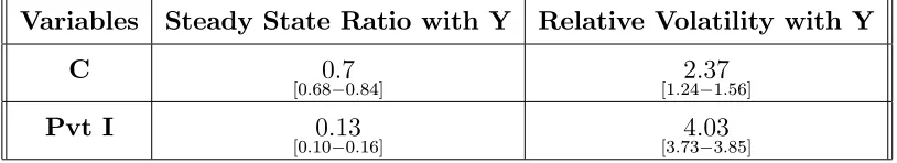
Tables 3a and 3b below present some preliminary results. We can see that steady state results of the model are either very close or within the empirical range of the data. The empirical range here are the minimum and the maxi-mum values of the series over a decade during the data period from 1980-81 to 2009-10. As far as the relative volatility of consumption and investment with output are concerned, our model overestimates these statistics as compared to the data.

Table 3a: Steady State Ratios and Relative Volatility2

Variables Steady State Ratio with Y Relative Volatility with Y

C 0:7

[0:68 0:84] [1:24 12:37:56]

Pvt I 0:13

[0:10 0:16] [3:73 34:03:85]

The cross-correlations of consumption and private investment with output obtained from the model are also higher vis-a-vis data. The autocorrelations of output and investment are lower while it is higher for consumption. However, all of these moments are not too far from the range obtained for the relevant moment from the data.

On the whole we can say that our model performs reasonably well on the basis of these criteria and is in line with acceptable performance for DSGE models in the literature.

We can see that most signi…cant deviations from the data moments of relative volatility and cross correlation with output occur with respect to

consump-2 _{Numbers in parenthesis are minimum and maximum values over di¤erent decades}

tion. This can be partly explained by the fact that there are doubts over the accuracy of private consumption data for Pakistan.

Table 3b: Auto/Cross Correlations3

Variables Y C Pvt.I

Y 0:56

[0:62 0:69]

C 0:97

[0:52 0:78] [0:26 00:47:43]

Pvt.I 0:86

[0:56 0:70] [0:46 00:34:57]

In the national income accounting system of Pakistan, private consumption is actually treated as a residual (also pointed out in Baqai, 1965). This point is discussed in detail in Choudhary and Pasha (forthcoming) and Malik (forth-coming).

5.2 Response of Economy to Structural Shocks

After the assessment of the simulation performance of the model, the next step is to use the model for policy analysis i.e. to analyze the impulse response functions generated in response to di¤erent exogenous structural shocks in our model. In our simulation exercises, we include three shocks namely technology; …scal or government spending and interest rate shocks.

Figure 1, shows that following a positive technology shock in the formal sector (where technology lies by design), investment, output and consumption in the formal sector rise, while in‡ation falls. Since output rises, wages and working hours also rise and as a result there is an overall rise in household’s income. On the other hand output in the informal sector falls instantly but tends to rise in the subsequent periods. Similar is the behaviour of the labor hours of the informal sector.

3 _{Numbers in parenthesis are minimum and maximum values over di¤erent decades}

5 10 15 20 0

0.005 0.01

y

5 10 15 20 0

0.02 0.04

y_f

5 10 15 20 -2

0 2x 10

-3 _{y_i}

5 10 15 20 0

5x 10 -3 _c

5 10 15 20 0

0.01 0.02

c_f

5 10 15 20 -2

0 2x 10

-3 _{c_i}

5 10 15 20 -2

0 2x 10

-3 _{h_f}

5 10 15 20 -2

0 2x 10

-3 _{h_i}

5 10 15 20 0

2 4x 10

-3 _h

5 10 15 20 0

0.005 0.01

w

5 10 15 20 0

0.005 0.01

w_f

5 10 15 20 0

0.005 0.01

w_i

5 10 15 20 0

0.02 0.04

i

5 10 15 20 -0.02

0 0.02

pi

5 10 15 20 -0.01

0 0.01

R

Figure 1: IRFs of the Technology Shock

Labor hours increase in the formal sector, however, the magnitude is small i.e. due to the advancement in technology labor productivity increases which then cancels out the demand for extra labor arising due to higher formal consumption.

The informal sector’s wage rate risies instantly after the shock resulting from the spillover e¤ect of an initial increase in demand for labor in the formal sector (it is due to the income e¤ect resulting from higher formal consumption due to initial increase in demand of labor and rise in the wage rate). Later the wage rate declines and follows that of the formal sector.

Since in our model, the link between formal and informal sectors is modeled in a way that they interact mainly through consumption, and technology only e¤ects the formal sector, the intensity of the impact of the technology shock on informal consumption and informal wage is minor and is only in form of spillover from the formal sector through income e¤ect …rst and then through a convergence oriented substitution e¤ect of consumption.

In response to a positive shock to government spending (see …gure 2) the nominal rate of return increases making it di¢cult for the private formal …rms to invest in capital. This is the crowding-out e¤ect of government spending on private investment and is experienced more intensely by the formal producers who need to raise capital on their own. To this extent the informal sector (i.e. informal production) is una¤ected by crowding-out as their production process only utilizes labor and hence has no role for capital, however, spillovers remain.

This crowding-out results in lower level of aggregate output which then lowers aggregate wage with a certain lag of time. However, initially, hours worked and wages rise in the formal sector. This rise in wages is only for a short duration after which they fall below the steady state level.

5 10 15 20 -0.1

-0.05 0

y

5 10 15 20 -0.05

0 0.05

y _f

5 10 15 20 -0.2

-0.1 0

y _i

5 10 15 20 -0.2

-0.1 0

c

5 10 15 20 -0.2

-0.1 0

c_f

5 10 15 20 -0.2

-0.1 0

c_i

5 10 15 20 0

0.05 0.1

h_f

5 10 15 20 -0.2

-0.1 0

h_i

5 10 15 20 0

0.05 0.1

h

5 10 15 20 -0.01

0 0.01

w

5 10 15 20 -0.01

0 0.01

w_f

5 10 15 20 -0.01

0 0.01

w_i

5 10 15 20 -0.5

0 0.5

i

5 10 15 20 -0.2

0 0.2

pi

5 10 15 20 -0.05

0 0.05

R

Figure 2: IRFs of the Fiscal Shock

Over time, the overall income of the household falls, consumption falls, and as a result output falls below the steady state, making demand for labor lesser than supply for labor. The in‡ationary rise in government spending makes formal goods more expensive.

hours of the informal sector. However, the wage level of the informal sector is also subject to spillovers from the formals sector.

The results of …scal shock leading to crowding-out of private investment have also been empirically veri…ed for Pakistan (see Khan and Khan, 2007; and Ahmad and Qayyum, 2008).

5 10 15 20 -2

0 2x 10

-4 _y

5 10 15 20 -2

-1 0x 10

-4 _{y _f}

5 10 15 20 -2

0 2x 10

-4 _{y _i}

5 10 15 20 -2

-1 0x 10

-4 _c

5 10 15 20 -5

0 5x 10

-4 _{c_f}

5 10 15 20 -2

0 2x 10

-4 _{c_i}

5 10 15 20 -2

0 2x 10

-4 _{h_f}

5 10 15 20 -2

0 2x 10

-4 _{h_i}

5 10 15 20 -5

0 5x 10

-4 _h

5 10 15 20 -4

-2 0x 10

-4 _w

5 10 15 20 -4

-2 0x 10

-4 _{w_f}

5 10 15 20 -4

-2 0x 10

-4 _{w_i}

5 10 15 20 -2

0 2x 10

-3 _i

5 10 15 20 -5

0 5x 10

-3 _pi

5 10 15 20 -0.02

0 0.02

R

Figure 3: IRFs of the Interest Rate Shock

but only for a short period. This immediate and strong response of in‡ation is due to ‡exible prices, a feature of Pakistan economy in an annual setting.

Aggregate consumption also declines. This behavior is rational since house-holds substitute consumption for investment in bonds issued by the govern-ment, whereas private investment in the formal …rms decline due to relatively higher interest rate.

Consumption at sectoral level increases with an insigni…cant size and for shorter period after which it starts decreasing and becomes negative. The sudden positive jumps in the level of formal and informal consumption in re-sponse to monetary policy shock are inconsistent with empirical evidence on consumption which generally is in the form of aggregate consumption only. We …nd no suitable explanation for such behavior of these sector speci…c impulse responses.

Our results are generally consistent with Batini, et al. (2011) for Indian econ-omy, and especially for sector speci…c consumption. The policy impact on informal sector are small in size and shorter in duration as the policy rate is not directly linked with the production process in the informal sector. The response by the informal sector variables is only due to spillover e¤ects from formal sector, mainly coming from the household’s consumption decisions, as explained earlier. Generally, on aggregate level, the direction of impulse re-sponses from all three shocks is in line with existing literature (see Smets and Wouters, 2003).

6 Conclusion

In this paper we develop a general equilibrium model with an informal sector and three types of shocks. The theoretical moments of the model perform reasonably well for private investment and less so for consumption. The latter is to be expected as private consumption and is treated as a residual in the aggregate resource constraint equation of the national accounting system of Pakistan. Further probing reveals that per capita consumption from aggregate data and surveys on household consumption do not match. Consequently, empirical claims on consumption have to be taken with a pinch of salt.

Appendix

A Parameter Estimation

Discount Rate ( )

The discount rate has been estimated using annual data from 1981 2011. Return on government bonds and change in CPI have been used to measure long term interest rate and in‡ation respectively. To incorporate expectations, lagged in‡ation has been used to calculate the real interest rate.

Elasticity of Substitution Between Formal and Informal Labour (#)

In order to estimate #, we used the micro-level data from the annual Labor Force Surveys. We compiled labor force survey data from the last several waves available between 1997-98 and 2008-09. The survey was not conducted in 2000-01, 2002-03 and 2004-05.We estimated the elasticity of substitution between formal and informal sector separately for each wave (as well as for all the data compiled together). We ran the following regression as in Psacharopoulos and Hinchli¤e (1972):

ln W

F t

WI t

!

=a+#ln L

F t

LI t

!

where WF

t & WtI are the hourly wage rates of formal and informal sector

employees in a household. LF

t & LIt are the average hours worked in a week

by employees in the formal and informal sector respectively. A caveat for our estimation of elasticity of substitution between formal and informal labor is that we were limited by the nature of LFS being a household survey. Our sample was reduced signi…cantly for estimation by the fact that we could only use data from households that have more than one employee as well as at least on each in the formal and informal sector.

accounts (as asked in the next question of the survey “Does the enterprise keep written accounts?”). On the other hand employees that responded to the enterprise question with either Individual Ownership, Partnership or Other and also answered the written accounts question with either “No” or “Don’t know” were considered part of the informal sector.

Taylor Rule ( _t and Y t )

To obtain response of policy interest rate to deviations of in‡ation and output from steady state, we regress log of interest rate on deviations of in‡ation and output from their trend values. We use average call money rate, GDP de‡ator and per capita real GDP for interest rate , in‡ation and output. Deviation of in‡ation from steady state is measured using residuals of following estimation:

ln t =c+ t

Results of this estimation showc=0.087331 implying steady state gross in‡a-tion equal to 1.09. For deviain‡a-tion of output from steady state, we regress log of per capita real GDP on constant and trend through following equation and take residuals:

lnYt=c+ t+ Yt

Furthermore, to estimate the response of interest rate to deviations in in‡ation and output, we estimate following equation:

lnRt =c+ t 1+ Y Yt 1

Estimated responses to in‡ation and output deviations are then normalized as ₊ Y and

Y

+ Y to yield values of 0.48 for and 0.52 for

y

.

Shock Process ( A, G, R; A, G; R)

The TFP series is obtained by using residuals of estimated neo- classical pro-duction function thorough following regression:

lnYt= lnKt+ (1 ) lnLt+ lnAt

To estimate A, we estimate the following equation:

lnAt=c+ AlnAt 1+uAt

A is calculated using residuals of above equation. Owing to unavailability

inventory method. There are di¤erent ways to calculate capital stock series and parameters of technology shock process are sensitive to variations in capital stock series. Using di¤erent series, we get a range of estimates for A between

0.85-0.95 and A 0.0095-0.025. From these ranges, we choose the values of

0.9 and 0.02 for A and A respectively. Similarly, to obtain G and G, we

estimate the following equation:

lngt=c+ Glngt 1+ gt

Using log of real per capita government consumption, estimation of the above yield values of 0.78 for G. Standard deviation of residuals from above

regres-sion yields estimate of G that is 0.14. The parameters of the interest rate

shock, i.e., R and R have been estimated in the similar manner as well.

However, we have used the residuals of the Taylor Rule instead the simple AR-1 formulation followed for the other two shocks. The values obtained for

B Complete Model

Financial assets optimization equation

1

ct

= (1 +Rt)Et

1

t+1ct+1

Physical assets optimization equation

Et

"

t+1

(1 +Rt)

n

(1 ) +rk

t+1 o#

= 1

Aggregate hours worked optimization equation

ht=

wt

ct

1

Money holding optimization equation

Mt=Pt

= 1

ct

Et

1

t+1ct+1

Capital accumulation equation

kt+1 = (1 )kt+it

Supply of formal labour

hFt =

wF t

wt

!1

#

ht

Supply of informal labour

hI

t = (1 )

wI t

wt

!1

#

ht

Composite wage rate

wt =

"

wFt

1+# #

+ (1 ) wIt

1+# #

# #

Informal wage rate PI t Pt = w I t

Formal wage rate

wF

t = w

I t where, = 1 !

Formal price level

PF t

Pt

= 1

(1 ) " 1 mc

F t

General price equation

Pt1 =! PtF

1

+ (1 !) PI

t

1

Formal consumption

cF t =!

PF t Pt ! ct Informal consumption

cIt = (1 !)

PI t

Pt

!

ct

Gross general in‡ation rate

t =

Pt

Pt 1

Gross sectoral in‡ation rates

F t = PF t PF t 1 and I t = PI t PI t 1

Formal production function

yF

t =atkt hFt1

Marginal cost

mcF t =

1

at

( ) (1 ) (1 ) wF

t

1

rk t

Informal production function

yI t = h

I t

Taylor type rule

Rt= tr t t

! 1

yt

yt

! 2

Fiscal budget constraint

Gt+T Rt+

(1 +Rt)Bt 1

Pt

= YF ₊ Bt

Pt

+ Mt Mt 1

Pt

Formal and informal sectors’ aggregate resource constraints

yF

t =cFt +it+gt

yIt =c I t

Economy wide aggregate resource constraint

yt=cFt +c I

C Complete Model in Steady State

Financial assets optimization equation

R= 1

Physical assets optimization equation

n

(1 ) +rko_{= 1}

Hours worked optimization equation

h= w

c

1

Money holding optimization equation

M=P =

1

c

1

c

Capital accumulation equation

i= k

Supply of formal labour

hF = w

F

w

!1

#

h

Supply of informal labour

hI = (1 ) w

I

w

!1

#

h

Composite wage rate

w=

"

wF

1+# #

+ (1 ) wI

1+# #

# #

1+#

Informal wage rate

wI = P

I

Formal wage rate

wF = wI

General price equation

P1 =! PF 1 _{+ (1 !) P}I 1

Formal consumption

cF _=! P F

P

!

c

Informal consumption

cI _{= (1 !)} P I

P

!

c

Gross general in‡ation rate

= 1

Formal production function

yF =k hF1

Capital-labour ratio

k hF = ₁

wF

rk

Marginal cost

mcF = ( ) (1 ) (1 ) wF

1

rk

Formal price

PF = 1

(1 )

"

" 1 M C

F

Informal production function

yI _{= h}I

Demand for informal labour equation

PI

P =W

Taylor type rule

R=r 1 y

y

! 2

Formal and Informal sectors’ aggregate resource constraints

yF _=cF _+i+g

yI _=cI

Economy wide aggregate resource constraint

D Complete Model in the Log-linearized Form

Financial assets optimization equation

e

ct = RRft+cgt+1+ gt+1

Physical assets optimization equation

Et gt+1 RRft = rkrgkt+1

Hours worked optimization equation

f

ht=

1

(wft cet)

Money holding optimization equation

e

ct = (1 ) M~t+ ~Pt Et(~t+1+ ~ct+1)

Capital accumulation equation

e

kt= (1 )kgt 1+ iet

Supply of formal labour

f hF t == 1 # g wF

t wft +fht

Supply of informal labour

f hI t = 1 # f wI

t wft +fht

Composite wage rate

f

wt=

1

w1+##

wF

1+# # g

wF

t + (1 ) wI

1+# # f

wI t

!

Informal wage rate

f

wI

t =PftI Pft

Formal wage rate

g

wF t = (

1)

f

wI t

Formal price level

~

PtF Pft =mcgFt

Informal price level

f

wI

General price equation

f

Pt=! PgtF + (1 !) PftI

Formal consumption

f

cF

t = PgtF Pft +cet

Informal consumption

e

cI

t = PftI fPt +cet

Gross general in‡ation rate

ft=Pft Pgt 1

Formal production function

f

yF

t = ket+ (1 )hfFt +aet

Capital-labour ratio

f

kF

t =wgtF +hfFt frtk

Marginal cost

g

mcF

t = frkt + (1 )wgFt aet

Informal production function

f

yI t =hfIt

Taylor type rule

~

Rct = 1ft+ 2yet+ et

f

yF t =

1

yF

h

cFcfF

t +iiet+get

i

yt=

1

y

h

cFcfF

t +cIceIt +iiet+get

i

Gross general in‡ation rate

References

Ahmad, I. and Qayyum, A. (2008), "E¤ect of Government Spending and Macro-Economic Uncertainty on Private Investment in Services Sector: Ev-idence from Pakistan", European Journal of Economics, Finance and Admin-istrative Sciences, Issue 11.

Ahmed, W., Haider, A. Iqbal, J. (Forthcoming), "A Guide for Developing Countries on Estimation of Discount Factor and Coe¢cient of Relative Risk Aversion", State Bank of Pakistan Working Papers.

Aksoy, Y., Basso, H. S. and Martinez, J. C. (2009), "Lending Relationships and Monetary Policy", Birkbeck Working Papers in Economics and Finance.

Andersen, T. M. (1998),"Persistency in Sticky Price Models”, European Eco-nomic Review, Papers and Proceedings, 42, 593-603.

Antunes, A. and Cavalcanti, T. (2007), "Start up Costs, Limited Enforcement, and the Hidden Economy", European Economic Review, 51, 203-224.

Arby, M. F., Malik, M. J., and Hanif, M. N. (2010), "The Size of Informal Economy in Pakistan", State Bank of Pakistan, Working Paper 33.

Aruoba, S. (2010), "Informal Sector, Government Policies and Institutions", Mimeo, University of Maryland.

Aruoba, S. and Schorfheide, F. (2011), "Sticky Prices versus Monetary Fric-tions: An Estimation of Policy Trade-o¤s"’ American Economic Journal, 60-90.

Baqai, M. U. (1965), "The Use of National Income Accounts in Planning Com-mission in Pakistan", Middle Income Studies in Income and Wealth, edited by Tau…q M. Khan, Bowes and Bowes Publishers, London.

Batini, N., Levine, P., Lotti, E., and Yang, B. (2011), "Informality, Frictions and Monetary Policy”, Discussion Papers in Economics, University of Surrey.

Castillo, P. and Montoro, C. (2008), "Monetary Policy in the Presence of Informal Labour Markets", Mimeo, Banco Central de Reserve del Peru.

Chari, V. V., Kehoe, P. J., and McGrattan, E. R. (2000), “Sticky Price Mod-els of the Business Cycle: Can the Contract Multiplier Solve the Persistence Problem?”, Econometrica, 68(5), 1151-1180.

Christensen, I., and A. Dib (2008): “The Financial Accelerator in an Estimated New Keynesian Model,” Review of Economic Dynamics, 11(1), 155–178.

Choudhary, A., Naeem, S., Faheem, A., Hanif, N. and Pasha, F. (2011), "For-mal Sector Price Discoveries: Preliminary Results from a Developing Coun-try", SBP Working Papers Series, No. 42.

Choudhary, A., Naeem, S. and Ahmed, W. (Forthcoming), "Formal Sector Wage Discoveries: Evidence from a Developing Country", State Bank of Pak-istan Working Papers.

Choudhary, A., and Pasha, F. (Forthcoming), "Modeling Pakistan: A First Step", Mimeo.

Collard, F. and Dellas, H. (2004). "The New Keynesian Model with Imperfect Information and Learning,". Mimeo, CNRS-GREMAQ.

Conesa, J. C., Diaz-Moreno, C., and Galdon-Sanchez, J. E. (2002), "Explain-ing Cross-Country Di¤erences in Participation Rates and Aggregate Fluctua-tions", Journal of Economic Dynamics and Control, 26, 333-345.

DiCecio, R., and Nelson, E. (2007), “An Estimated DSGE Model for the United Kingdom”, Federal Reserve Bank of St. Louis Working Paper Series, Working Paper 2007-006B.

Edge, Rochelle M. (2002), "The Equivalence of Wage and Price Staggering in Monetary Business Cycle Models," Review of Economic Dynamics, 5(3), 559-585.

Fabrizio, M. and Lorenz, R. (2010), "Optimal Monetary Policy in Economies with Dual Labor Markets", Journal of Economic Dynamics and Control, 33(7), 1469-1489.

Fagan, G., and Messina, J. (2009), “Downward Wage Rigidity and Optimal Steady State In‡ation”, European Central Bank, Working Paper Series, Work-ing Paper 1048.

Fuhrer, J. C., (2000). "Habit Formation in Consumption and Its Implications for Monetary-Policy Models", American Economic Review, 90(3), 367-390.

Gali, J. (1994), "Monopolistic Competition, Business Cycles, and the Compo-sition of Aggregate Demand", Journal of Economic Theory, 63, 73-96.

Huang, K. X. D. and Liu, Z. (2002), "Staggered Contracts and Business Cycle Persistence”, Journal of Monetary Economics, 49, 405-433.

Khan, S. A. and Khan, S. (2011), “Optimal Taxation, In‡ation and the Formal and Informal Sectors”, State Bank of Pakistan, Working Paper Series, Working Paper 40.

Khan, S. and Khan, M. A. (2007), "What Determines Private Investment? The Case of Pakistan", PIDE Working papers, 2007:36.

King, R. G. and Rebelo, S. T. (1999), “Resuscitating Real Business Cycles” in Handbook of Macroeconomics, Vol. 1B, edited by John B. Taylor and Michael Woodford.

Koreshkova, T. (2006), "A Quantitative Analysis of In‡ation as a Tax on the Underground Economy", Journal of Monetary Economy, 773-796.

Kremer,J., Lombardo, G., von Thadden, L., and Werner, T. (2006), “Dynamic Stochastic General Equilibrium Models as a Tool for Policy Analysis”, Eco-nomic Studies, Oxford University Press, 52(4), 640-665.

Kydland, F. and Prescott, E. (1982), "Time to Build and Aggregate Fluctu-ations”, Econometrica, 50, 1345-1370.

Liu, S. (2008), "Capital Share and Growth in Less Developed Countries”, China Centre for Economic Research.

Malik, M. J. (Forthcoming), "Mismatch between Household Survey and Na-tional Account Consumption Data Sets", State Bank of Pakistan Working Papers.

Pichler,P. (2007), “Forecasting with Estimated Dynamic Stochastic General Equilibrium Models: The Role of Non-linearities”, Department of Economics, University of Vienna, Working Paper 0702.

Psacharopoulos, G. and Hinchli¤e, K. (1972), “Further Evidence on the Elas-ticity of Substitution among Di¤erent Types of Educated Labour”, Journal of Political Economy, 80, 786-792.

Rotemberg, J. and Woodford, M. (1997), “An Optimization-based Econo-metric Framework for the Evaluation of Monetary Policy”, NBER Macro-economics Annual, 12. 297-346.

Smets, F. and Wouters, R. (2005), "Comparing Shocks and Frictions in US and Euro Area Business Cycles: A Bayesian DSGE approach”, Journal of Applied Econometrics, 20, 161-183.