Aggregate efficiency and interregional equity: a contradiction?

Aggregate efficiency and interregional

equity: a contradiction?

Alexiadis, Stilianos

15 June 2012

Aggregate Efficiency and Interregional Equity: A Contradiction?

Stilianos Alexiadis*

Ministry of Rural Development & Foods,

Department of Agricultural Policy & Documentation, Division of Agricultural Statistics

Room 501, 5 Acharnon Street, 101 76, Athens, Greece, Tel: ++30 210 2125517, E-mail: ax5u010@minagric.gr, salexiadis7@aim.com

Abstract

This paper attempts to rekindle interest on regional allocation of investment and to

show that a trade-off between aggregate efficiency and interregional equity is implied.

Modifying, however, the objective function it is established that this trade-off can be

avoided.

JEL Classification: R10

1. Introduction

A major concern for policy-makers is how to allocate resources across space (regional

investment) in order to achieve aggregate efficiency (maximum output) without

increasing regional inequalities (interregional equity). The purpose of this paper is to

contribute in that direction using Optimal Control Theory (hereafter OCT) and

amending the framework developed by Intriligator (1964). The rest of the paper is laid

out as follows. Section 2 summarises what we can learn from the model of regional

allocation of investment. Section 3 then outlines an alternative framework, modifying

the objective function by attaching a „weight‟ in each region. Section 4 summarises

the arguments and considers the lessons for policy making.

2. Regional Allocation of Investment

A starting point is provided by Intriligator (1964), who building upon the work of

Rahman (1963), showed that OCT can be applied in order to maximise national

output (Y_N ) in a „two-region‟ economy at some terminal time (T ). Given a

*

production function Y_i v_iK_i, i 1,2, fixed capital coefficient and assuming that a constant proportion of output is saved (S_i s_iY_i), capital accumulation evolves as

2 2 1 1 2

1 K K K

K  1. Intriligator (1964) assumes that once capital is placed in one region, it cannot be shifted into the other region. Total savings are pooled in a central

agency and allocated to each region, given an „allocation parameter‟ ( ). The

objective function is, therefore,MaxY_N(T), subject to the constraints, given by

equations (1), (2) and (2) below.

)

( _{1 1 2 2}

1 K K

K (1)

) )(

1

( _{1 1 2 2}

2 K K

K (2)

1

0 (3)

Assuming constant returns, at any point in time either *(t) 0 or *(t) 1, The problem can be solved by identifying the value of (t) that maximises the

Hamiltonian function, H [ (p₁ p₂) p₂]( ₁K_{1 2}K₂), where p₁and p₂are the auxiliary variables, frequently referred to as the implicit price of capital. The optimal

path of depends on the sign of the difference p₁(t) p₂(t). Put simply, the optimal solution suggests that the funds should be invested in the region where the shadow

price of capital is higher. Thus, if p₁(t) p₂(t) 0, then * 1 while if 0

) ( )

( ₂

1 t p t

p , then * 0. The Hamiltonian system must satisfy the conditions

} , {

max _{1 2}

1 1

1 p p

K H

p and ₂ max{ ₂, ₁}

2

2 p p

K H

p , implying that

1 2 2 1

1 [ (p p ) p ]

p and p₂ [ (p₁ p₂) p₂] ₂. Therefore,

2 2 1 2 2

1(t) p (t) p (t)

p (4)

The auxiliary variables must satisfy the terminal conditions 1

1 1 ) ( ) ( ) ( v T K T Y T p N and 2 2 2 ) ( ) ( ) ( v T K T Y T

p N . Given that

2 1 2 1 ) ( ) ( v v T p T p , then 2 2 1 2 2

1( ) ( ) ( )

v v v T p T p T

p (5)

1

For a given planning period, [0T], *(t) 1 at 0 t T if _{1 2}or *(t) 0 if

2

1 . Conversely, at t T invest only in the region with the highest output/capital

ratio; that is to say if v₁ v₂, then *(t) 1 while if v₁ v₂, then *(t) 0. Following Takayama (1967), setting 0 yields p₂ p_{2 2}, which is a first order differential equation with the solution _{p2(t) v2e} 2(T t)_{. Solving for t, the switching}

time can be estimated:

1 2 1

2 1 2

*

log 1

v s s T

t (6)

In the model so far, the possibility of uneven distribution of regional incomes is not

considered, at least explicitly. Nevertheless, a number of interesting implications can

be derived. In order to have a concrete vocabulary, define the initial income gap

between region 1 and 2 as G(0) Y₁(0) Y₂(0). Assuming that G(0) 0, _{1 2} and v₁ v₂, then the optimal solution *(t) 1, ∀t∈ [0T] yields maximum output but at the expanse of closing the income „gap‟ between region 1 and 2, i.e. a

trade-off between aggregate efficiency and regional equity. When _{1 2} and v₁ v₂

a switch in the allocation parameter is necessary if total output is to be maximised.

This will also reduce regional inequalities at t T2. A steady elimination of the income gap between the two regions while a constant increase in total output is

feasible if _{1 2} and v₁ v₂. Given that v₁ v₂ and _{1 2}, the solution 0

) (

*

t ,∀t∈[0T], enables the planner to overcome the trade-off between efficiency and equity3.

Nevertheless, it is possible to extend the argument by attaching a „weight‟ in each

region. While Takayama (1967) acknowledges that this possibility, nevertheless, to

the best of our knowledge, this remained a rather unexplored area and is examined in

the next section.

2

If 1 2 and v1 v2, then () 0 * _t

at0 t T and *(_t) 1

at t T . Regional disparities can be reduced at 0 t T and increase again at the end of the period.

3

Similarly, the trade-off is absent when *() 1

3. Regional Allocation of Investment: An Alternative Perspective

According to Intriligator (1964), the investment decision is determined exclusively by

different growth potentials in each region. It is possible, however, to attach a different „weight‟ to each region4

, reflecting political or social reasons. National output,

therefore, can be expressed as: YN(T) iYi(T), where i 0 is the weight attached to each region5. Maintaining OCT as the basic vehicle of analysis, the problem is

defined as ) ( ) ( )

(T ₁v₁K₁ T ₂v₂K₂ T Y

Max _N , with _{1 2} 0 (7)

subject to the constraints defined by equations (1), (2) and (3).

It follows that

2 2 1 2 2

1(t) p (t) p (t)

p while the terminal conditions

1 1 1(T) v

p and p₂(T) ₂v₂, imply that

2 2 2 2 1 1 2 2

1( ) ( ) ( )

v v v T p T p T

p (8)

Before the end of the planning period (0 t T) the optimal solution is *(t) 1 if

2

1 or ( ) 0 *

t if _{1 2}. At the end of the planning period (T ) if ₁v_{1 2}v₂, then *(t) 1 while if ₁v_{1 2}v₂, then *(t) 0. The switching time is given by the following expression:

2 2 1 1 2 1 1 2

2 ( )

) (

log

1 s s v

T

t (9)

Essentially, the objective function in equation (7) encapsulates two components,

aggregate efficiency and interregional equity. When G(0) 0 and _{1 2}, the

efficiency component dominates. By analogy, if G(0) 0 and _{1 2}, then the

equity element is of primary concern6. Nevertheless, the aim G(T) 0 might not be

feasible. Hence, it would be more reasonable to define an aim G(T) 0. The

4_{The notion of „region‟ can be extended to include groups of geo}

graphical areas. Just as an example

consider „agricultural‟ and „industrial‟ regions or „northern‟ and „southern‟ regions.

5

From a technical standpoint attaching weights (

n

i i

1

1) does not alter the structure of the

production functions.

6

investment sequence when _{1 2} and _{1 2}are set out in Table 1 and 2,

respectively.

Table 1: Regional Allocation of Investment when _{1 2}

_{1 2 1 2}

2 1 v

v v₁ v₂ v₁ v₂ v₁ v₂

2

1 1 2 0 1 2 0 1 2 0 1 2 0

) ( )

( 2

1T p T

p 1v1 2v2 0 1v1 2v2 0 1v1 2v2 0 1v1 2v2 0

) (

*

t at0 t T 1 1 0 0

) (

*

t at t T 1 1 1 1

Table 2: Regional Allocation of Investment when _{1 2}

_{1 2 1 2}

2 1 v

v v₁ v₂ v₁ v₂ v₁ v₂

2

1 1 2 0 1 2 0 1 2 0 1 2 0

) ( )

( 2

1T p T

p 1v1 2v2 0 1v1 2v2 0 1v1 2v2 0 1v1 2v2 0

) (

*

t at0 t T 1 1 0 0

) (

*

t at t T 0 0 0 0

Table 1 implies that if G(0) 0 and _{1 2}, then the optimal policy sustains the

initial gap in regional incomes, provided that _{1 2}. A change in the allocation

parameter triggers a reduction in regional inequalities if _{1 2}. Assume, however,

that G(0) 0 and that the planner has an explicit interest in reducing the income gap

between the two regions. This assumption can be expressed as _{1 2}7. According

to the conditions set out in Table 2, *(t) 1 at 0 t T if _{1 2}. Given that

2

1 , then ( )=0

*

t

δ at t=T, irrespective of the difference in the capital

coefficients. In this case, although initial regional disparities increase during the

period 0 t T, a reduction in the income gap between the two regions is possible due to a switch in at t=T. While Intriligator (1964) implies a trade-off when

2

1 and v1 v2, this can be avoided by imposing 1 2. Contrary to the

possibility of perpetuating regional inequalities, implied by Intriligator (1964) when

1 ) (

*

t , t [0T]. It is conceivable that regional equity dominates when _{1 2} and _{1 2}. The allocation parameter remains unchanged and a steady elimination

7

of the income gap is observed. The optimal solution implied by the conditions _{1 2}

and _{1 2} is *(t) 0, t [0T]. Thus, irrespective of the productivity differences between regions, a simultaneous reduction of regional inequalities and

maximisation of aggregate output is possible. In terms of the analysis by Intriligator

(1964) this is feasible only if v₁ v₂ and _{1 2}.

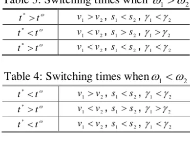
Table 3 and 4 compare the switching times implied by equation (6) and (9) when

2

1 and 1 2, respectively.

Table 3: Switching times when _{1 2}

t t*

2 1 v

v , s₁ s₂, _{1 2}

t t*

2 1 v

v , s₁ s₂, _{1 2}

t t*

2 1 v

v , s₁ s₂, _{1 2}

Table 4: Switching times when _{1 2}

t t*

2 1 v

v , s₁ s₂, _{1 2}

t t*

2 1 v

v , s₁ s₂, _{1 2}

t t*

2 1 v

v , s₁ s₂, _{1 2}

4. Conclusion

An aggregate efficiency and regional equity component is normally involved in the

design of regional policies. Nevertheless, these might contradict each other, given that

maximising aggregate efficiency may increase regional income differentials; a topic

that appears to be attracting increasing attention and interest amongst policy-making

bodies. This paper has shown that this contradiction can be avoided by a simple

modification of the model, developed by Intriligator (1964). Introducing, a weight to

the income of each region, provides a range of policies which result to a simultaneous

reduction of regional inequalities and maximisation of total output, allowing for a

more efficient allocation of scarce resources. Nevertheless, this depends on the time

horizon and the chosen spatial units. The variation discussed in this paper is versatile

and flexible enough to be applied in various contexts and provides a range of choices

to policy-makers in designing regional (or even sectoral) policies. Yet, economic

knowledge cannot be gleaned from theory alone. For theoretical innovation to

convince they need to be evaluated through observed facts. This clearly implies the

need for more detailed and focused analysis and research before the trade-off can be

main purpose should be to provoke interest and further discussion in the possibility of „bridging‟ the gap between aggregate efficiency and interregional equity.

References

Intriligator, M. (1964) “Regional Allocation of Investment: Comment”, Quarterly Journal of Economics, 78(4), 659-662.

Rahman, A. (1963) “Regional Allocation of Investment: An Aggregate Study in the

Theory of Development Programming”, Quarterly Journal of Economics, 77 (1), 26-39.

Takayama, A. (1967) “Regional Allocation of Investment: A Further Analysis”,