Munich Personal RePEc Archive
Pro poor growth : A partial ordering
approach
Sarkar, Sandip
Indian Statistical Institute Kolkata
9 May 2014
Pro poor growth : A partial ordering approach
Sandip Sarkar
Economic Research Unit, Indian Statistical Institute.
203, B. T. Road, Kolkata 700108, India.
9th May, 2014
Abstract
The paper examines the partial pro poor orderings for different
growth curves and sets of Equally Distributed Equivalent growth rate
dominance. A new pro poor growth curve as the of change of Gini
social welfare function, based on the quantiles of logarithmic income,
has been proposed. It has been established that the newly proposed
growth curve including its relative version i.e its deviation from the
growth rate of mean, is robust to other growth curves that has been
proposed in the literature, in terms of conclusiveness. Empirical
illus-trations are provided using Monthly per capita expenditure data, for
different states of India, officially collected by National Sample Survey
Office. It has been observed that the absolute and relative versions
provides conclusive result in many cases where other pro poor growth
curves fails to do so. Growth in rural and urban India is pro poor in
an absolute sense, since from the early 1990s. Although, relative pro
poor growth has been achieved for some spells in rural India, but, in
Urban India, it is in general biased to the non-poor in most of the
spells.
Key words: Pro Poor Growth; Stochastic dominance; Inequality;
India
1
Introduction
Most of the developing economies show evidence of increment of growth rate
over the last few decades. Questions have been raised by academicians and
policy makers, whether poorer section of the society enjoys the benefit from
it. Thus the concept of pro poor growth evolved, mainly, to analyze the fact,
whether growth is favorable to the poor or not.
The notion “pro poor growth” might be analyzed by two different senses.
In general growth is said to be pro poor in an absolute sense, if it raises income
of the poor, or poverty declines See Kraay (2006) . Following Kakwani and
Pernia (2000), growth is labelled as “pro-poor” in a relative sense, only if it
raises the incomes of poor proportionately more than that of the non poor.
Osmani (2005), criticized, both these approaches.1 He proposed a stronger
absolute definition of pro-poor growth, that growth is pro poor if the poverty
reduction is higher than the benchmark level. However, establishing such a
benchmark is not easy and is always debatable. On the other hand, this is
also a relative approach, which can be traced back to Kakwani and Pernia
(2000).
Both, absolute and relative pro poor growth might also be evaluated with
two alternative ordering approaches, viz complete and partial ordering
ap-proach. Any ordering satisfying reflexivity, transitivity, and completeness
property is a complete ordering approach.2 For example, as a result of
incre-ment of average income, if head count ratio declines, growth is said to be pro
poor in an absolute sense. The main problem of this approach is it ignores
1According to Osmani, ‘‘simply reducing poverty cannot, in general, be a sufficient
condition for pro-poorness....In that sense, Kakwani’s definition is a move in the right di-rection. He calls a growth process pro-poor only when the poor benefit proportionately more than the rich. But he takes the bias to an extreme, leading to potentially counterintuitive implications.” (Osmani,2005).
the fact that choice of a different poverty index, or a different poverty line
might alter the result. Partial ordering pro poor growth on the other hand
relaxes the completeness axiom. Although situations might end
inconclu-sively, but conclusions if provided is robust to the choice of different class of
index and/or parameter used to compute those index.
Partial pro-poor ordering begins with the contribution of Ravallion and
Chen(2003). They proposed Growth Incidence Curve (GIC), which measures
the rate of change of income quantile. A conclusive result is obtained
follow-ing GIC, if it lies strictly above zero for at least one quantile and not below
zero for any of the quantiles. Son (2004) developed a new approach on the
basis of Atkinson (1987) theorem linking the generalized Lorenz curve and
changes in poverty, and proposed a new growth rate curve namely poverty
growth curve (PGC). GIC and PGC provides conclusive result if there is
evi-dence of first and second order stochastic dominance of one distribution over
the other respectively. Since, Stochastic dominance conditions are nested,
PGC provides better results than GIC, in terms of conclusiveness. A
rela-tive version of GIC and PGC are derived considering their deviations from
the average growth rate of the society. Recently, Duclos (2009) suggested
a relative pro poor orderings approach, based on normalizing income of all
individuals by any pro poor standard.
Adopting a complete ordering approach, Nssah(2005) introduced a
con-cept called Equally distributed Equivalent Growth rate(EDEGR). EDEGR is
almost similar to equally distributed equivalent income introduced by
Atkin-son (1970), as the growth rate socially equivalent to observed one, for some
choice of a focal parameter, which measures the degree of inequality aversion.
EDEGR might also be represented as weighted average of the points of the
type. Nassah also defined Distributive Adjusted Factor (DAF), considering
the deviation of EDEGR from the growth rate of mean. She declared that
absolute and relative pro poor growth occurs in the society, when EDEGR
and DAF respectively are strictly positive.
Our first objective in this article is to relax the restrictions on the weights
adopted by Nssah. We begin by introducing a concept called EDEGR
domi-nance. EDEGR dominance is obtained, if EDEGR is non negative for a class
of the weights attached, and strictly positive for at least one of those weights.
The choice of the class of the weights is based on some ethical restrictions
on EDEGR, which we believe a pro poor growth index must satisfy. The
restrictions are based on weak monotonicity, Transfer principle(PT) and
po-sitional version of transfer principle (PPTS) , discussed in details by Zoli
(1999). Accordingly, we have first, second and third order EDEGR
domi-nance. Further, third order EDEGR dominance of one distribution over the
other, implies growth is pro poor following the class of EDEGR following
Nssah. Since, EDEGR is weighted average of all income quantile, our
do-main of interest will be logarithmic income. We have shown that the EDEGR
dominance and inverse stochastic dominance (ISD) based on logarithmic
in-come domain are equivalent. The nested property of ISD implies dominance
conditions derived in this article are also nested. Hence, the third order
EDEGR dominance is the most general one, and theoretically it is possible
to construct situations where it provides conclusive results, unlike others.
In order to apply the third order EDEGR dominance empirically, we have
further introduced a new growth curve based on gini social welfare function.
In spite of the fact that, the newly proposed growth curve is based on
log-arithmic income domain, we have shown that conclusive GIC and/or PGC
the newly proposed growth curve. We have also characterized the relative
version of EDEGR i.e DAF, using the normalization approach suggested by
Duclos (2009). Thus if we consider a domain with income of all individuals
being normalized by their mean, we obtain DAF dominance almost similar to
EDEGR dominance. Further, we have shown that DAF dominance implies
(implied by) EDEGR dominance when the avearge growth rate of the society
is positive (negative).
The paper has been organized in the following fashion. The next section
consists of discussion on some preliminary topics, related to this article. In
section 3 we have introduced the new dominance result. An empirical analysis
has been done in section 4. The first part of the empirical analysis deals with
the performance of new growth curve in terms of conclusiveness. The second
part is mainly to evaluate the pro poor scenarios of India for the last two
decades. The paper is concluded in section 5.
2
Preliminaries
In a society, let at time point t and t-1, yt = (y1t, y2t...ynt) ∈ Rn++, and
yt−1 = (y
t−1
1 , y2t−1...ymt−1)∈Rm++, be the vector of incomes arranged in
ascend-ing order. Through out this paper our aim is to evaluate whether movement
of income profile yt−1 to yt is pro poor or not. Let Ft(y) be the
empiri-cal distribution function, representing percentage of individuals with income
≤y. In some cases we will also represent the distribution function as F(yt),
where yt denotes the underlying domain of the distribution function.
Con-sider ypt = F−1
t (p) = inf{y : Ft(y) ≥ p} as the pth income quantile of the
income distribution at time point t. Let, µt =
R1
0 y
p
tdp, be the mean income
rate.3
2.1
Stochastic and inverse stochastic dominance
If yt is defined on a continuum, the recursive integral for the distribution
function may be written as Ftr+1(y) =
Ry
0 F
r
t(s)ds ∀s ∈[0,∞) where r ≥0
is an integer. Stochastic Dominance (SD) and Inverse Stochastic Dominance
(ISD) has remained one of the major tolls of partial ordering approaches,
including partial pro poor ordering analysis. We will discuss these issues
very briefly. Our main analytical results also depends on these techniques.
Definition 1. Stochastic dominance : F(yt) stochastically dominates
F(yt−1) by r+1 th order/degree i.e F(yt)≻r+1 F(yt−1) if Ftr+1(s)≤F r+1
t−1(s) ∀ s ∈[0,∞) & < for at least one s.
Instead of considering a distribution function, the same purpose might be
solved using the inverse distribution function. LetF−(r+1)
t (p) =
Rp
0 F
−(r)
t (p)dp
where r≥0 is an integer.4
Definition 2. Inverse Stochastic dominance : F(yt)dominatesF(yt−1)
by (r+1)th order/degree Inverse Stochastic Dominance i.e F(yt) ≻−(r+1)
F(yt−1) if F −(r+1)
t (p)≥F−
(r+1)
t−1 (p) ∀p∈[0,1] & > for at least one p.
SD and ISD are nested, i.e lower order implies higher order dominance.
However, the reverse is not necessarily true. SD implies ISD and vice versa
for r ≤ 2. However, for r > 2 the relationship is no longer valid. SD of
one distribution over the other implies a decline of poverty for a class of
poverty index discussed in Atkinson(1987). SD also implies an increment of
3The operator ∆ will denote the the difference of the function between time point t
and t-1; e.g ∆xt= (xt−xt−1) 4For expressions ofFr+1
t (y) andF
−(r+1)
welfare for different class of social welfare functions also known as “Welfare
Dominance”, SeeFoster and Shorrocks (1988a,b).
2.2
Absolute and Relative Pro poor growth
We will now formally introduce the concepts of absolute and relative pro
poor growth. In a nutshell a growth is said to pro poor in an absolute sense
if it raises the income of the poor Kraay (2006). It may also be defined as
follows
Definition 3. Absolute Pro Poor growth : A change from yt to yt−1
is said to be pro-poor in an absolute sense whenever, as a result of growth,
poverty declines.
Considerg >0, and for a given poverty index and poverty line, if poverty
declines we would say growth is pro poor in an absolute sense, following a
complete pro poor ordering approach. The absolute pro poor growth might
be accessed by considering the growth elasticity of poverty, which measures
the % change in poverty as a result of increment of 1% growth. Thus following
the above definition if the elasticity is negative, growth might be considered
as pro poor.
It is possible that pro poor growth ordering might depend on choice of
poverty indexes and/or ordering. In order to rule out these inconsistencies,
Ravallion and Chen (2003), considered a partial ordering approach based
on first order SD and proposed Growth Incidence Curve (GIC). GIC is the
rate of change of ytp, which can be represented as GIC(p) = ∆log(y p t). If
GIC(p) ≥ 0 ∀ p & > 0 for at least one p we refer the situation as pro
poor growth or GIC(p) ≻ 0. Whereas GIC(p) ≤ 0 ∀ p & < 0 for at
Son (2004) considered poverty growth curve (PGC) on the basis of second
order stochastic dominance. The proposed growth curve is the rate of change
of generalized lorenz curve of two distributions, P GC = ∆log(µpt), where µ p t
might also be interpreted as the mean of poorest 100p% of population. Since,
GIC and PGC are respectively based on first and second order stochastic
dominance, conclusive ordering of these curves would also imply decline of
poverty for a wide range of poverty index. The ordering is also robust to the
choice poverty line.
Kakwani and Pernia (2000) introduced the concept of relative pro poor
growth, where the focus is mainly based on the income growth rate of the
poor. The formal definition may be written as follows
Definition 4. Relative Pro poor growth : A movement from yt to yt−1
is said to be pro poor in a relative sense, if the growth rate of income of poor
is greater than that of the non poor.
It should be noted that the above definition remains unchanged, even if
we simply replace “growth rate of the non poor”, by the average growth rate
of the society. A relative version of GIC and PGC might be related to Lorenz
curves. The relative versions of GIC and PGC might be written as follows
g1 = GIC−g = ∆L′t(p)
g2 = P GC −g = ∆Lpt (1)
where Lpt and L′t(p) stands for lorenz curve and slope of lorenz curve
respectively. Thus growth is pro poor following GIC and PGC in a relative
sense, if and only if the slope of the lorenz curve and lorenz curve does not
normalization approach suggested by Duclos(2009). If we normalize income
of all individuals at time point t and t−1 by their respective means and
denote the domains ¯yt and ¯yt−1 respectively, it can be shown that GIC and
PGC ordering, will essentially lead to g1 and g2 ordering, where
¯
yt = {y1t/µt, y2t/µt, ..ytn/µt}
¯
yt−1 = {y
1
t−1/µt−1, y
2
t−1/µt−1, ..y
n
t−1/µt−1} (2)
It should be noted that the approach suggested byDuclos(2009) is more
general in the sense that the normalization is not necessary to be by the
mean. It may be any summary statistics, which the policy maker is
actu-ally interested in, e.g Median, Percentiles e.t.c. However, for the sake of
simplicity, we consider the normalization by mean, mainly to track Kakwani
and Pernia (2000) definition. We will discuss more on this issue when we
introduce our dominance results.
2.3
Equally Distributed Equivalent Growth Rate
Nssah (2005) considered a complete ordering approach and defined Equally
Distributed Equivalent Growth Rate(EDEGR) as growth rate socially
equiv-alent to the observed growth for some choice of the focal parameter which
cap-tures the degree of inequality. EDEGR might be considered as the weighted
average of the points of GIC
ζ =
Z 1
0
v(p)∆log(ytp)dp=λ¯v 1−
cov ∆˜ytp, v(p)
−λv¯
!
(3)
where v(p) is the weight attached to pth quantiles and ¯v = R1
Nssah considered weights as v(p) = v(1−p)v−1, where v is an indicator of
aversion of inequality. The choice of specific weight function leads to ¯v = 1,
thus from equation 3,ζ takes the form of EDEGR, almost similar to Equally
distributed as proposed by Atkinson (1970). However, for any choice of
weight function w(p) =v(p)/v¯, EDEGR might be obtained from 1 provided
¯
v 6= 0, and finite.
Thus from 3we can write
ζ∗ =λ 1− cov ∆˜y
p t, w(p)
−λ
!
(4)
A relative version of EDEGR might also be obtained following its
devia-tion from the average growth rate. Nassah termed it as distributed adjusted
factor (DAF).
DAF = ζ∗−g
=
Z 1
0
w(p)∆log(ytp/µt)dp (5)
It is possible to obtain the DAF dominance, similar to g1 and g2
order-ing, by considering the normalization approach suggested by Duclos(2009).
However, we have to consider a logarithmic transformation of all the points
of domain ¯yt and ¯yt−1. Let the new domain is defined as ¯lt and ¯lt−1, where
¯
lt = {log(yt1/µt), log(y2t/µt), ..log(ytn/µt)}
¯
lt−1 = {log(y
1
t−1/µt−1), log(y
2
t−1/µt−1), ..log(y
n
t−1/µt−1)} (6)
nor-malization should necessarily be mean income of the society. This also leads
DAF as the weighted average of the rate of change of slopes of the Lorenz
curve.
3
A new dominance result
In this section we will introduce a new dominance result, based on the
re-strictions of the weight function on an ethical point of view. Since, EDEGR
is weighted average of all income quantile, our domain of interest will be
logarithmic income denoted by ˜yt = {log(y1t), log(y2t)...log(ynt)}. Essentially
we establish relationship between EDEGR dominance and inverse stochastic
dominance based on this domain.5 Before introducing the dominance
re-sults and discussing on the restrictions necessary on the weight function, we
formally introduce the concept of EDEGR dominance as follows.
Definition 5. EDEGR Dominance : For a class of weightsWR ∈W that
satisfies properties R, EDEGR dominance occurs whenζ∗(w)≥0 ∀w ∈W
R
and ζ∗(w)>0 for at least one w∈W
R or ζ∗(w)≻0.
3.1
Restrictions on EDEGR
For the sake of simplicity, we will consider only the class of weight function
which is differentiable. The first restriction we would like to impose is similar
to the monotonicity property of a poverty index. We will consider the case,
such that, if there is positive growth for at least one quantile given other
quantiles remains unchanged, growth rate must not be anti pro poor. Let x
be the growth profile consisting of all the points of GIC, and xi denotes the
5The results are motivated from Zoli’s work on inverse stochastic dominance and welfare
GIC for the ith quantile. Let Dn denotes the set of all growth profiles and
N = {1,2..n} denotes the set of integers of order n, where n is the number
of quantiles.
Axiom 1. Week monotonicity (WM) : ∀x ∈ Dn, ∀ i, j ∈ N, x j >
0, &xi ≥0, ∀j =6 i =⇒ EDEGR(x)≥0.
The second restriction is essentially on the line of transfer axiom as
pro-posed in the inequality literature. It is likely that in a society, a rank
pre-serving progressive (regressive) transfer of income from the richer to poorer
quantile, would lead to an increase (decrease) of EDEGR.6 The definition of
rank preserving transfer might be formally written as follows7
Definition 6. Rank preserving Transfer(RPT) : Let x, z ∈ Dn be
the growth profiles, x is obtained from z by a rank preserving Transfer, if
for some i, j (i < j) & xl = zl, ∀l 6= {i, j}, xi −zi = zj −xj = δ, where
δ ≤ zj−zi
2 if j =i+ 1 and δ ≤min{(zi+1−zi),(zj−zj−1)} if j > i+ 1.
The transfer is progressive and regressive ifδ >0 andδ <0 respectively.
Let x(i, j) denotes that in a growth profile x, a RPT takes place from j to i.
The transfer is progressive and regressive if j > i and j < i, respectively.
Axiom 2. Week Transfer principle (PT) : ∀x∈ Dn, ρ ∈ N and 1<
ρ < n, EDEGR(x, x+ρ)≥EDEGR(x)andEDEGR(x+ρ, x)≤EDEGR(x)
Our next axiom will be introduced mainly to consider the fact that
trans-fer will be valued more if it takes place at the bottom of the distribution.
Axiom 3. Week Principle of positional version of Transfer
sen-sitivity(PPTS) : ∀x ∈ Dn, ρ, i, l ∈ N and 1 ≤ ρ ≤ n−l, i < l, then
6It is difficult to imagine the transfers between the quantiles. However, using this axiom,
comparison of pro poor growth performances between different societies is possible.
EDEGR x(i, i+ρ)
≥ EDEGR x(l, l+ρ)
and EDEGR x(i+ρ, i)
≤
EDEGR x(l+ρ, l)
.
We will use the following lemma that essentially establish the relationship
between the weights function of EDEGR and the axioms discussed above.
Lemma 1. Any twice differentiable EDEGR satisfies WM if w(p)>0,
sat-isfies PT if w′(p)≤0 and satisfies PPTS if w′′(p)≥0.
Consider the following class of weight functions for which EDEGR satisfies
different axioms.
w1(p) = {w(p)∈W :w(p)≥0} (7)
w2(p) = {w(p)∈W :w(p)≥0 & w′(p)≤0} (8)
w3(p) = {w(p)∈W :w(p)≥0, w′(p)≤0 & w′′(p)≥0} (9)
Forw1 EDEGR satisfies WM, for w2 WM and PT and lastly forw3 WM,
PT an PPTS. Using the above set of weight functions, we will now introduce
our first main result of the article, that essentially establish a partial ordering
of EDEGR dominance.
Theorem 1. ζ∗(w
i)≻0iff F(˜yt)≻−i F(˜yt−1)∀i∈ {1,2,3}and additionally
λ ≥0 for i=3.
Whereλ is the growth rate of geometric mean. Even if λ <0, but ˆg ≻0,
EDEGR dominance is obtained. For example, if one sets weights for the
richest quantile as 0 i.e w4 = {w(p) ∈ W : w(p) ≥ 0, w′(p) ≤ 0, w′′(p) ≥
0 and w(1) = 0} then ˆg ≻ 0 ⇒ ζ∗(w
4) ≻ 0. Weights adopted by Nssah is
a subset of w4. It should be further noted that since ISD are nested, would
imply EDEGR dominance derived in this article are also nested. Thus our
Corollary 1. Higher order EGEDR dominance implies lower order
domi-nance, however, the reverse is essentially not true.
It is important to emphasize that, the 3rd order EGEDR dominance, will
be most robust in terms of conclusiveness. For the empirical application of
the third order EDEGR dominance, we will introduce a new pro poor growth
curve.
3.2
A new pro poor growth curve
The dominance result derived in the previous section, essentially are based
on ISD on log transformed incomes. The empirical applications of the first
and second order EDEGR dominance might be easily obtained constructing
GIC and PGC on this domain. For application of the third order EDEGR
dominance, we propose a new growth curve as the change of gini social
wel-fare functions of logarithmic income for the poorest 100p% of population.
The gini social welfare function also known as Sen’s welfare function, is
the product of mean and one minus gini coefficient thus captures notions
of both equity and efficiency. Thus the new growth curve is written as
ˆ
g = ∆wpt = ∆˜µ p t(1−˜g
p
t), where w p t, ˜µ
p
t and ˜g p
t are the gini social welfare
function, mean and gini coefficient respectively of logarithmic incomes for
the poorest 100p% of population. We will use a result of Zoli(1999) in order
to establish relationship between ISD and ˆg.
Lemma 2. If gˆ≻0 ⇐⇒ F(˜yt)≻−3 F(˜yt−1)
Our next target is to relate GIC, PGC and ˆg ordering. Since, the domain
of the first two curves are different from that of ˆg, we will consider our next
the relationship between SD and Welfare dominance byFoster and Shorrocks
(1988a,b), which we consider as our next Lemma.
Lemma 3. F(yt) ≻−2 F(yt−1) =⇒ 1
R
0
u(yt)dF >
1
R
0
u(yt−1)dF where u is
differentiable and u′ >0 and u′′ <0 (Foster and Shorrocks, 1988a,b)
Using the above Lemma8, we derive a new lemma, which basically relates
the EDEGR dominance on log transform domain and income domains.
Lemma 4. GIC ≻ 0 ⇐⇒ Ft(˜yt) ≻−1 Ft−1(˜yt−1) and P GC ≻ 0 ⇒
Ft(˜yt)≻−2 Ft−1(˜yt−1)
Using Lemma 4 and nested property of ISD, it can be shown that PGC
ordering might be considered as a sufficient case for ˆg ≻ 0. However, the
reverse is not true, thus the new growth curve provides conclusive results in
many cases where both GIC and PGC fails to do so. Hence,
Proposition 1. If P GC ≻0⇒gˆ≻0
Although, the new growth curve provides conclusive results in cases the
PGC fails to do so. However, it should be noted that unlike PGC where pro
poor growth and poverty indexes might be related, it is not possible for the
new growth curve. The rationale, for the choice of this curve, is that the
third order EDEGR dominance is obtainable using the new growth curve. A
conclusive ˆg ordering is sufficient to say that growth is pro poor at least for
the class of EDEGR as suggested by Nssah.
8For income domain being continuous the result was derived in Foster and Shorrocks
3.3
Relative Pro-poor growth
So far our discussion was based on the absolute notion of pro poor growth. It
is possible to extend the dominance condition also in the context of relative
pro poor ordering. Similar to EDEGR dominance, DAF dominance might
also be considered provided domain is considered as ¯lt (See equation6).
Let ¯ltp, denotes thepthquantile based on ¯lt. Thus the next theorem
essen-tially establish relationship between DAF dominance and inverse stochastic
dominance on the domain ¯lt. Like third order EDEGR dominance an extra
condition is also required for DAF dominance β = R1
0 ∆¯l
p
tdp ≥ 0, which
again can be relaxed for choice of w4.
Theorem 2. For any EDEGR with weights being wj, DAF(wj) ≻ 0 iff
Ft(¯lt)≻−j Ft−1(¯lt−1)∀j ∈1,2andDAF(w3)≻0iff Ft(¯lt)≻−3 Ft−1(¯lt−1)and
β ≥0.
Like the EDEGR dominance results our next corollary will essentially
imply DAF dominance is also nested.
Corollary 2. DAF(W1)≻ 0⇒DAF(w2)≻ 0⇒DAF(w3)≻ 0.
The third order DAF dominance is the most general in terms of
con-clusiveness. It might be obtained by computing ˆg on ¯lt, or might also be
accessed by considering the curve g3 = ˆg −g. The g3 curve might also be
related to g1 and g2 defined in 1.
Proposition 2. g1 ≻0 =⇒ g2 ≻=⇒ g3 ≻0.
Essentially the proposition shows that g3 might conclude in many
situ-ations where g1 and g2 fails to do so. A conclusive ordering of the gi curve
We will now investigate on the relationship between DAF dominance
and EDEGR dominance. Our next proposition essentially says that DAF
dominance is a sufficient condition for EDEGR dominance if the growth rate
of mean g > 0. On the other hand, DAF dominance will always hold if
EDEGR dominance occurs provided g <0. Hence our next proposition
Proposition 3. If g > 0, DAF ≻ 0 =⇒ EDEGR ≻ 0 and if g <
0 EDEGR ≻0 =⇒ DAF ≻0.
In the next section we will consider the performances absolute and relative
versions of GIC, PGC and the newly proposed growth curves empirically.
4
Empirical analysis
Our aim in this section is twofold. Firstly, using major states of rural and
urban India, we will analyze the performances of GIC, PGC and ˆg along
with their relative versions g1, g2 and g3. Secondly, we will discuss on pro
poor scenarios of rural and urban India, mainly for the last two decades.
We will use National Sample survey Office (NSSO) data on consumer
expen-diture. Under the program, the survey on consumer expenditure provides
a time series of household consumer expenditure data, which is the prime
source of statistical indicators of level of living, social consumption and
well-being, poverty estimation e.t.c. NSSO does not collect data on income, thus
expenditure is considered to be a proxy. We shall use monthly per-capita
ex-penditure(MPCE), based on mixed recall period method. In a mixed recall
period method in India, data for educational, medical (institutional),
cloth-ing, beddcloth-ing, footwear and durable goods are collected on a recall period of
30 days.9 In this article we will use consecutive rounds data on consumer
expenditure vij 43rd, 50th, 55th, 61st and 66th, which provides information’s
respectively for the period of July 1987 - June 1988, July 1993 - June 1994,
July 1993 - June 1994, July 1999- June 2000, July 2004-June 2005, and July
2009-June 2010. In order to account for the price adjustments, we have
ad-justed MPCE of rural India using consumer index for agricultural labourer
(CPIAL), whereas consumer price index for Industrial workers(CPIIW) for
urban India.10 For both the state and all India level of rural and urban India
the number of quantile is 20.
4.1
Pro poor evaluation in states of India
We will evaluate the performance of both absolute and relative versions of
GIC, PGC and the newly proposed growth curves, using 20 states for rural
India and 17 for Urban states of India. The number of years considered in
this study is 5. We consider all possible combinations of state and year, thus
we have altogether 4950 and 3570 pairs of distribution respectively for rural
and urban India.
For each states, we compute GIC, PGC and ˆg following the five
consec-utive NSSO rounds. In Table 1, we have reported the number of pro poor,
anti poor, inconclusive and inconsistent conclusive (IC) cases along with the
percentage of conclusive cases (CC). IC refers to the number of cases where
9Comparison in terms of survey design is same for all the rounds. However, 55th
rounds contains information of both 7 days and 30 days recall period and is likely to create problems in comparability issues. See Deaton et al Deaton and Kozel (2005). Although there are several methodologies available for the adjustments of this recall error, we will not consider these issues for the sake of simplicity.
10The same procedure was also used in adjustments of poverty line estimation in India.
lower order dominance provides conclusive result but the higher order fails
to do so. Theoretically this is not possible, it arises due to choice of small
number of income quantiles.11 If the number of quantiles is increased
sub-stantially, the conclusive results as shown by GIC and/or PGC in these cases
eventually turns out to be inconclusive.
The last column of Table 1 refers to the percentage of conclusive cases,
excluding IC. GIC provides conclusive statements nearly about 40% cases in
both rural and urban India. However, the performance of its relative version
g1 is very poor and provides less than 1% cases in both rural and urban
India. PGC on the other hand provides conclusive statements on 80% cases,
but its relative version performs poorly and more than 40% cases remains
as inconclusive. The performance of the newly proposed growth curve is not
only better in terms of the absolute sense but also in a relative sense. For
both the cases more than 80% cases are concluded.
Insert Table 1 here.
4.2
Pro poor evaluation in Rural and Urban India
Our target in this part is to see whether the evidence of sustained GDP
growth in India is favorable to the poor or not. Growth process started
mainly on the 1990s when liberalization took place in India, and policies
changed substantially at that point.12 Using NSSO data for the last five
11It has been observed that for all these cases the inconsistency arises at the lowest
quantiles.
12In the 1980’s India lacked the confidence of international community on her economic
quinquennial rounds, we will evaluate the pro-poor scenarios of India for all
possible spells of comparison of rural and urban India. Since, one of our
data point is before 1990 (43rd round), we thus also have the opportunity to
evaluate pro poor scenarios before and after liberalization.
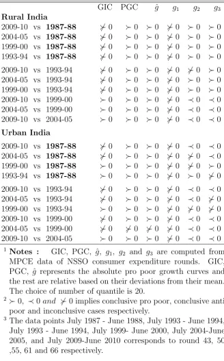
All comparison results has been provided in Table2. It is readily
observ-able that, for both rural and urban India, growth is pro poor in an absolute
sense, following PGC and ˆg. GIC fails to provide conclusive results in
al-most all cases. However, it has been observed that in alal-most all the cases
inconsistency arises due to a negative value in the last quantile. Since, the
last quantile in GIC is the growth rate of the maximum values, there is
ev-ery possibility that the inconsistency arises due to presence of outliers in the
data.13
Following g3, it has been observed for any comparison of other rounds
with the pre liberalization period, growth is pro poor in relative sense in the
rural India. The conclusion remains same even if we simply replace the data
point by just after the period of liberalization i.e 1993-94. However, for the
remaining spells of comparisons, growth is favorable to the rich.
Pro poor scenario in urban regions of India, are almost opposite to that
of her rural regions. Here, we get six out of the ten cases as anti pro poor
in a relative sense. Only in one case i.e. for 55 th vs 43 rd round, following
g3 we found growth is pro poor in a relative sense. However, since there are
comparability problems of the 55th round data, this result should be reported
with caution. An example of inconsistent conclusive case might be observed
in the comparison of 55 vs 43 round. In this case although the relative PGC
provides conclusive result, but the newly proposed fails to do so. Perhaps a
13The inconclusive situations of GIC, might be concluded using a technique called
better way to deal this situations is to consider different statistical tests for
Stochastic dominance that has been proposed in the literature. We consider
this as our future research plan.
Insert Table 2 here.
5
Conclusion
Nssah(2005) introduced the concept of equally distributed equivalent growth
rate (EDEGR) as the growth rate socially equivalent to the observed one for
some choice of focal parameter capturing the degree of inequality. EDEGR
appeared to be the weighted average of points og the growth incidence curve
(Ravallion and Chen, 2003). However, the weights were restricted to the
relative extended Gini type class of functions. A relative version of it, also
known as distributed adjusted factor(DAF), was also proposed in the same
article as the deviation from growth rate of mean.
Our main contribution in this article is to introduce a partial ordering
con-dition for EDEGR and DAF, which we have termed as EDEGR and DAF
dominance. The dominance results derived in this article, are based on
ethi-cal restrictions, which we assume a pro poor growth index must satisfy. The
first order EDEGR (DAF) dominance corresponds to the satisfaction of week
monotonicity property of pro poor index, i.e if growth is positive in at least on
quantile, growth must not be anti poor. For the second order EDEGR(DAF)
dominance an additional transfer principle has been incorporated, which
im-plies is transfer of income from richer to poorer quantile growth rate will
be pro poor. Additionally we need principle of positional version of
trans-fer sensitivity for third order EDEGR dominance. It states that transtrans-fer is
condi-tions are based on inverse stochastic dominance on log transformed income
distribution. Thus the conditions are nested i.e lower order EDEGR(DAF)
dominance will always imply higher order, but the reverse is not necessarily
true. The EDEGR chosen by Nssah, satisfies all these properties and we have
shown that if there is evidence of third order dominance of one distribution
over the other, EDEGR will be pro poor.
Since, the third order dominance curve is most general in terms of
conclu-siveness, we have introduced a new growth curve for its empirical application.
The growth curve corresponds to the change of gini social welfare function
based on the quantiles of logarithmic income. It provides conclusive result if
and only if there is evidence of third order inverse stochastic dominance of
one distribution over the other (Zoli, 1999). However, the domain has to be
modified by considering a log transformation of income of all the individuals.
Previously there has been evidence of two growth curves Growth incidence
curve (GIC) and Poverty growth curve (PGC) based on first and second
or-der stochastic dominance. It has been established in spite of the fact that the
domain of the growth curves being different, a conclusive statement of GIC
and/or PGC would always imply the same for the new growth curve.
How-ever, it is possible to construct situations where unlike the previous curves,
the newly proposed curve provides conclusive statements.
The same analysis might also be extended for the context of relative pro
poor comparison. However, it is necessary to change the domain by
con-sidering normalization of incomes by any pro poor standard (Duclos,2009).
For the sake of simplicity and for DAF dominance we consider the pro poor
standard as the mean income of the society.
The performance of the newly proposed growth curve and its relative
(MPCE) data for rural and urban regions of Indian states. We have used data
for five consecutive NSSO quinquennial rounds, for the period of 1987-88,
1993-94, 1999-00, 2004-05 and 2009-10. For each data points we have further
divided into 20 and 17 major states of rural and urban India respectively. Our
results shows that the absolute and relative version of the newly proposed
growth curve provides conclusive results nearly in 80% of the cases. The
absolute and in particular the relative version performs much better than
the same for PGC and eventually for GIC.
Another empirical exercise has also been considered mainly to analyze
whether the growth process started in the early 1990s is pro poor or not.
Instead of considering subgroups of Rural and Urban Indian states, this
ex-ercise is based on the full sample of rural and urban India. Thus for the five
data points we have 10 spells of comparisons separately for each sectors. It
has been observed that, growth is in general pro poor in an absolute sense in
both rural and urban India, for all the spells of NSSO rounds. Although we
have found some evidence of relative pro poor growth in the spells of rural
India, but mostly anti poor in urban India.
In the empirical analysis, we found that in a very few cases, lower order
dominance provides conclusive results, but higher order fails to do so. This
arises due to choice of low number of income quantiles, and the inconsistency
disappears once we increase the number of quantiles. We refer these cases as
inconsistent conclusive results. A future research program in this direction
will be to derive the asymptotic properties of the newly proposed curves, and
References
Atkinson, A.B. (1970), “On the measurement of inequality.” Journal of
Eco-nomic Theory, 2, 244–263.
Atkinson, A.B. (1987), “On the measurement of poverty.”Econometrica, 55,
749–764.
Chakravarty, S.R. (1990), Ethical Social Index Numbers. Springer Verlag,
New York.
Chakravarty, S.R. (2009), Inequality Polarization and Poverty. Advances in
Distributional Analysis. Springer Verlag, New York.
Deaton, A and V. Kozel (2005), “Data and dogma : The great indian poverty
debate.” The World Bank Research Observer, 20, 177–199.
Duclos, J. Y. (2009), “What is pro-poor?” Social Choice and Welfare, 58,
32–37.
Foster, J. E. and A. F. Shorrocks (1988a), “Poverty orderings.”
Economet-rica, 56, 173–177.
Foster, J. E. and A. F. Shorrocks (1988b), “Poverty orderings and welfare
dominance.”Social Choice and Welfare, 5, 179–198.
Kakwani, N. and E. Pernia (2000), “What is pro-poor growth?” Asian
De-velopment Review, 16, 1–22.
Kraay, A. (2006), “When is growth pro-poor ? evidence from a panel of
countries.”Journal of Development Economics, 80, 198–222.
Nssah, E.B. (2005), “A unified framework for pro-poor growth analysis.”
Osmani, S. (2005), “Defining pro-poor growth.” One Pager Number 9,
In-ternational Poverty Center, Brazil, 9.
Ravallion, M. and S. Chen (2003), “Measuring pro-poor growth.”Economics
Letters, 78, 93–99.
Son, H.H. (2004), “A note on pro-poor growth.” Economics Letters, 82, 307–
314.
Zoli, C. (1999), “Intersecting generalized lorenz curves and the gini index.”
6
Appendix
Proof of Theorem 1
Proof : Fori = 3 the proof is similar to Zoli (Zoli, 1999) on Yaris social
welfare function and ISD. We will prove for i={1,2}
Case 1 : i=1
(Sufficiency) If F(yt) ≻ F(yt−1) ⇐⇒ GIC ≻ 0 ⇐⇒ ∆log(ytp) ≻ 0,
since w(p) ≥ 0, thus ζ∗(w
1) =
R1
0 w(p)∆log(y
p
t)dp ≥ 0. Clearly if w(p) >
0 ∀p∈[0,1]⇒ζ∗ >0.
Necessary : We begin with the assumption, that, GIC fails to provide
conclusive results. Thus in interval u1 = (¯p,p¯¯)⊂ (0,1), GIC(p) <0∀p ∈u1
and >0∀p∈[0,1]−u1. Consider the following weight function
w(p) = a >0 ∀p∈(0,p¯)
= b >0 ∀p∈(¯p,p¯¯)
= c >0 ∀p∈(¯¯p,1)
Considering the weight structure mentioned above we get the following
expression for ζ∗ = aRp¯
0 ∆log(y
p
t)dp + b
Rp¯¯
¯
p ∆log(y p
t)dp + c
R1
¯ ¯
p ∆log(y p t)dp.
Clearly for b chosen very high and low compared to a and c, would lead
to ζ∗ < 0 and ζ∗ > 0 respectively. The last part F
t(˜yt) ≻−1 Ft−1(˜yt−1) iff
Ft(yt)≻−1 Ft−1(yt−1) is trivial and is left to the reader.
Case 2 : i=2
(Sufficiency) Integrating by parts ζ∗ we get
ζ∗ =
Z 1
0
∆log(ytp)dp−
Z 1
0
w′(p)
Z s
0
∆log(yts)ds
!
dp (10)
Ft(yt) ≻−2 Ft−1(yt−1)⇒
Rs
0 ∆log(y
s
the second term is always>0 given w′(p)≤0. Since the first term is always
positive whenever Ft(yt) ≻−2 Ft−1(yt−1) holds. Hence ζ∗ ≥ 0. Choosing
weights such that w′(p)<0∀p∈[0,1], would always lead to ζ∗ >0.
Sufficient : LetFt(yt)6≻−2 Ft−1(yt−1), consider the following weight
func-tions
w(p) = a−L1p >0 ∀p∈(0,p¯)
= b−L2p >0 ∀p∈(¯p,p¯¯)
= c−L3p >0 ∀p∈(¯¯p,1) (11)
where all the parameters a, b, c, L1, L2 and L3 are positive. From 10 we can
always getζ∗ <0 andζ∗ >0 for choice of high and low values ofL
2, provided
a, b, c L1 and L3 has been restricted accordingly. Hence EDEGR dominance
breaks.
Proof of Theorem 2
Proof : Similar to Theorem1.
Proof of Lemma 3 : FOr domain being continuous see Foster and
Shorrocks (1988a), while domain being discrete see Foster and Shorrocks
(1988b).
Proof of Lemma 4
Proof : The first part i.eGIC ≻0 ⇐⇒ ˆg ≻0 is trivial and is left to the
author.
For the second part essentially, have to showF(yt)≻F(yt−1)⇒F(˜yt)≻
F(˜yt−1). Consider, income profiles are discrete (for the sake of simplicity)
F(yt)≻F(yt−1)⇒ i X i=1 yi t≻ i X i=1 yi
t−1 (12)
Similarly, considering logarithmic income domain
F(˜yt)≻F(˜yt−1)⇒
i X i=1 ˜ yi t≻ i X i=1 ˜ yi t−1 ⇒
i Y i=1 yi t≻ i Y i=1 yi
t−1 (13)
We shall show 12⇒13, by method of induction. For n = 1, it would be
a trivial exercise. For n = 2, if 12 holds we can write
yt1 ≥ yt1−1 (14)
yt1+yt2 ≥ yt1−1+y
2
t−1 (15)
with strict inequality for at least one case.
Ify2
t−1 ≤y
2
t it would be once again a trivial exercise to show that yt1yt2 ≥
y1
t−1yt2−1. The maximum value of yt2−1, following 15 can written as zt2−1 =
y1
t +y2t −yt1−1. It can be shown
yt1yt2 ≥yt1−1zt2−1 (16)
whenever14holds. Clearly, if we consider any smaller value thanzt−1 the
inequality would always hold. For n= 3 the same results can also be proved
easily.
Without loss of generality assuming the equivalence is established for
n = k, where k is any integer and k > 3. We will establish the relationship
for n =k+ 1.
Clearly, the conditions implies a generalized Lorenz dominance of income
distribution t over t-1. Following Lemma 3 Pk+1
any x >0, u′(x) >0 & u′′(x) <0. Putting u(x) = log(x) satisfies both the
conditions. Hence we can write Pk+1
i=1(yti−yti−1)>0⇒
Qk+1
i=1 yti >
Qk+1
i=1 yit−1.
Hence proved.
If population size is not fixed, letym
t andytn−1 bemtimes replication of all
individuals of the first distribution andntimes replication of all individuals in
the second distribution. It is well known that stochastic dominance
relation-ship are replication invariant, thus Ft(yt)≻−r Ft−1(yt−1) ⇐⇒ Gt(ytm)≻−r
Gt−1(ytn−1), r being an integer. Thus the analysis again might be thought as
a comparison exercise on fixed population size.
Proof of Proposition 1
Proof : Following Lemma 4 we can write P GC ≻ 0 =⇒ F(˜yt ≻−2
F(˜yt−1). Since, ISD is nested F(˜yt≻−2 F(˜yt−1) =⇒ F(˜yt ≻−3 F(˜yt−1) =⇒
ˆ
g ≻0. Hence Proved
Proof of Proposition 2 Proof : Using nested property of ISD g1 ≻
0 =⇒ g2 ≻0. The last part is similar to Proposition 1, only domain being
different.
Proof of Proposition 3 Proof : The proof is easy, and might be
con-structed computing EDEGR on domain ¯lt defined on 6, which is eventually
Table 1: Performances for different growth curves
States of Rural India
Index Inconclusive Anti Poor Pro poor IC CC
GIC 2804 724 1422 173 39.86%
P GC 917 1121 2912 122 79.01%
ˆ
g 616 1171 3163 NA 87.56%
g1 4932 11 7 7 0.22%
g2 2084 946 1920 107 55.74%
g3 659 1434 2857 NA 86.69%
States of Urban India
Index Inconclusive Anti Poor Pro poor IC CC
GIC 2026 424 1120 85 40.87%
P GC 675 738 2157 77 78.94%
ˆ
g 418 915 2237 NA 88.29%
g1 3556 13 1 5 0.25%
g2 1532 1361 677 66 55.24%
g3 572 1886 1112 NA 83.98%
1 Notes : Results are based on spells of 20 major states
of Rural India and 17 major states of urban India for the July 1987 - June 1988, July 1993 - June 1994, July 1999-June 2000, July 2004-1999-June 2005, and July 2009-1999-June 2010. The results of pro poor conclusions are based on any two possible combinations of state and round. Thus we have altogether 4950 and 3570 pairs of distributions, for com-putation of the growth curves.
2 GIC, PGC, ˆg, g
1, g2 and g3 are computed from MPCE
data of NSSO consumer expenditure rounds. GIC, PGC, ˆ
g represents the absolute pro poor growth curves and the rest are their relative versions i.e. their deviations from their mean. The choice of number of quantile is 20.
3 IC represents inconsistent conclusive cases, due to low
Table 2: Pro poor growth scenarios in India
GIC PGC gˆ g1 g2 g3
Rural India
2009-10 vs 1987-88 6≻0 ≻0 ≻0 6≻0 ≻0 ≻0 2004-05 vs 1987-88 6≻0 ≻0 ≻0 6≻0 ≻0 ≻0 1999-00 vs 1987-88 6≻0 ≻0 ≻0 6≻0 ≻0 ≻0 1993-94 vs 1987-88 6≻0 ≻0 ≻0 6≻0 ≻0 ≻0 2009-10 vs 1993-94 6≻0 ≻0 ≻0 6≻0 6≻0 ≻0 2004-05 vs 1993-94 6≻0 ≻0 ≻0 6≻0 ≻0 ≻0 1999-00 vs 1993-94 6≻0 ≻0 ≻0 6≻0 ≻0 ≻0 2009-10 vs 1999-00 ≻0 ≻0 ≻0 6≻0 ≺0 ≺0 2004-05 vs 1999-00 ≻0 ≻0 ≻0 6≻0 ≺0 ≺0 2009-10 vs 2004-05 ≻0 ≻0 ≻0 6≻0 ≺0 ≺0
Urban India
2009-10 vs 1987-88 6≻0 ≻0 ≻0 6≻0 ≺0 ≺0 2004-05 vs 1987-88 6≻0 ≻0 ≻0 6≻0 6≻0 ≺0 1999-00 vs 1987-88 ≻0 ≻0 ≻0 6≻0 6≻0 ≻0 1993-94 vs 1987-88 ≻0 ≻0 ≻0 6≻0 ≻0 6≻0 2009-10 vs 1993-94 6≻0 ≻0 ≻0 6≻0 ≺0 ≺0 2004-05 vs 1993-94 6≻0 ≻0 ≻0 6≻0 ≺0 6≻0 1999-00 vs 1993-94 ≻0 ≻0 ≻0 6≻0 6≻0 6≻0 2009-10 vs 1999-00 6≻0 ≻0 ≻0 6≻0 ≺0 ≺0 2004-05 vs 1999-00 6≻0 6≻0 6≻0 6≻0 ≺0 ≺0 2009-10 vs 2004-05 ≻0 ≻0 ≻0 6≻0 ≺0 ≺0
1 Notes : GIC, PGC, ˆg, g
1, g2 and g3 are computed from
MPCE data of NSSO consumer expenditure rounds. GIC, PGC, ˆg represents the absolute pro poor growth curves and the rest are relative based on their deviations from their mean. The choice of number of quantile is 20.
2 ≻0, ≺0and 6≻0 implies conclusive pro poor, conclusive anti
poor and inconclusive cases respectively.
3 The data points July 1987 - June 1988, July 1993 - June 1994,