Munich Personal RePEc Archive
Local politics and economic geography
Berliant, Marcus and Tabuchi, Takatoshi
Washington University in St. Louis, University of Tokyo
15 May 2013
Local Politics and Economic Geography
Marcus Berliant
yDepartment of Economics, Washington University in St. Louis
Takatoshi Tabuchi
zFaculty of Economics, University of Tokyo
May 15, 2013
Abstract
We consider information aggregation in national and local elections when voters are mobile and might sort themselves into local districts. Using a
standard model of private information for voters in elections in combination with a New Economic Geography model, agglomeration occurs for economic reasons whereas voter strati…cation occurs due to political preferences. We
compare a national election, where full information equivalence is attained, with local elections in a three-district model. We show that full information
equivalence holds at a stable equilibrium in only one of the three districts
The authors thank Rod R. Blagojevich for inspiring this work. We are grateful to Yasushi Asako, Stefano Barbieri, Arnab Biswas, John Duggan, Gilles Duranton, Antoine Loeper, Teemu Lyytikäinen, Debraj Ray, Nathan Seegert, Alastair Smith, Razvan Vlaicu, and seminar audiences at the Public Choice Society meetings in San Antonio, the Wallis Institute at the University of Rochester, and the Econometric Society Winter Meetings in San Diego for helpful comments. We are grateful to the University of Tokyo for …nancial support, but we retain responsibility for any errors.
yDepartment of Economics, Washington University, Campus Box 1208, 1 Brookings Drive,
St. Louis, MO 63130-4899 USA. Phone: (314) 935-8486. Fax: (314) 935-4156. E-mail: berliant@artsci.wustl.edu
zFaculty of Economics, University of Tokyo, Hongo 7-3-1, Bunkyo-ku, Tokyo 113-0033, Japan.
when transportation cost is low. The important comparative static is that full information equivalence is a casualty of free trade. When trade is more costly,
people tend to agglomerate for economic reasons, resulting in full information equivalence in the political sector. Under free trade, people sort themselves
into districts, most of which are polarized, resulting in no full information equivalence in these districts. We examine the implications of the model using data on corruption in the legislature of the state of Alabama and in the Japanese
Diet.
Keywords and Phrases: information aggregation in elections,
informa-tive voting, new economic geography, local politics
JEL Classi…cation Numbers: D72, D82, R12
1
Introduction
“Meanwhile, the di¤erences between the parties have become so strong, and so sharply split across geographic lines, that voters may see their choice of where to live as partly re‡ecting a political decision. This type of voter self-sorting may contribute more to the increased polarization of Congressional districts than redistricting itself.” Nate Silver, 538 Blog, New York Times, December 27, 2012
We seek to address questions at the boundary of politics and geography: Under what circumstances do localities, such as cities, become politically polarized? How much information is revealed in local as opposed to national elections? Does the mobility of voters help or hinder information aggregation in local elections? Of course, the electorate is generally smaller in local as opposed to national elections, but does voter migration for economic reasons result in polarization of local elections?
is corrupt. In polarized districts, our model predicts that candidates with an ex-treme view that coincides with the electorate in their district will be elected whether they are corrupt or not, whereas in unpolarized districts fewer corrupt candidates are elected, as people vote using their signals as if they were pivotal. A complicating factor, that we shall address speci…cally in our model, is the mobility of consumers and their endogenous selection of district.
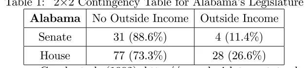
Consider the following data, collected by Couch et al. (1992), on whether Alabama state-elected o¢cials received income from serving on boards of local state-funded universities in 1987-1988. House districts are evidently smaller.
Table 1: 2 2 Contingency Table for Alabama’s Legislature
Alabama No Outside Income Outside Income Senate 31 (88.6%) 4 (11.4%)
House 77 (73.3%) 28 (26.6%)
Sources: Couch et al. (1992), http://www.legislature.state.al.us/
Note that House districts are not necessarily subsets of Senate districts.
2 = 3:46
Degrees of Freedom =1
Probability = 0:063
From this table we can see that the likelihood that House and Senate members di¤er in their receipt of outside income is large but not de…nitive. Could it be that some elections for the House imply more information aggregation than others?
[image:4.612.148.463.291.361.2]Table 2: 2 2 Contingency Table for Japan’s Diet1
Japan No Allegations Resigned Under Duress or Convicted House of Councilors 145 (99.3%) 1 (0.7%)
House of Representatives 289 (96.3%) 11 (3.7%) Source: http://www.notnet.jp/data04index.htm
Note that House of Representatives districts are subsets of House of Councilors districts.
2 = 3:33
Degrees of Freedom =1
Probability = 0:068
Again, there appears to be more corruption in elections involving smaller districts, but this is not de…nitive.
To address the theoretical questions we have posed as well as to explain the data, we formulate a model of politics and information aggregation in elections where voters are also economic agents and mobile. Geography and politics interact and feed back in interesting ways: On the one hand, economic factors might cause agglomeration of agents, thus a¤ecting the polarization of districts, the aggregation of information in local elections, and the outcomes of local elections. On the other hand, the outcomes of elections in localities might a¤ect the agglomeration of agents into these localities. This interplay leads us to the introduction of geography into models of politics, in particular those associated with the Condorcet jury theorem such as Austen-Smith and Banks (1996) and Feddersen and Pesendorfer (1997). It also leads us to introduce politics into models of strati…cation or agglomeration, such as Krugman (1991). In this respect, we could have used a model of local public goods for this purpose, but …nd the New Economic Geography model from urban economics to be both more tractable and less biased toward strati…cation. For example, in the US context, local education and quality of schools, along with property taxes, are the most important criteria used by consumers/voters for determining location of residence. Tiebout
1In the House of Councilors of Japan’s Diet, 146 of the 242 seats are elected in single-seat districts
sorting models will generally lead directly to strati…cation by type of consumer in equilibrium, implying a failure of full information equivalence (de…ned in the next paragraph) in the various districts. In summary, we could use a model of equilibrium in a local public goods economy in place of the New Economic Geography part of our model, but we conjecture that results would be similar. In general, New Economic Geography models lead to agglomeration, but not directly to strati…cation. We shall elaborate on this in the conclusions.
Our main …ndings are summarized as follows. We compare a national election, where the same outcome is attained whether voters know everyone’s private infor-mation or not (called full information equivalence2 in the political science literature),
with local elections in a three district model. We show that full information equiva-lence holds in only one of the three districts when transportation cost of goods is low. The important comparative static is thatfull information equivalence is a casualty of free trade. When trading goods is more costly, people tend to agglomerate for eco-nomic reasons, resulting in full information equivalence in the political sector. Under free trade, people sort themselves into three districts, two of which are polarized, resulting in no full information equivalence in these districts. The remaining district still satis…es full information equivalence. Thus, if the signals voters receive concern the con‡ict of interest or corruption of candidates in their district, it is expected that elections in districts with smaller populations (local elections) will result in a higher proportion of compromised elected o¢cials. This might even happen if the electorate is large, as in our model. But some of these districts will still satisfy full information equivalence, so the correlation between size of electorate and information aggregation in elections is imperfect. Nevertheless, our model endogenously generates politically polarized districts.
The literature on information aggregation in elections has a focus on an electorate that is exogenously given and thus is immobile. Austen-Smith and Banks (1996) presented the seminal work on the Condorcet jury theorem, showing in a game-theoretic context that for some states of nature, not all the information of voters is revealed in Nash equilibrium even if they all have the same objective functions and priors. Feddersen and Pesendorfer (1997) …nd su¢cient conditions for which full
information equivalence holds at Nash equilibrium, and that is the framework we employ below.
The literature on economic geography has almost no focus on voting, particularly when there is asymmetric information about candidates or ballot measures.
We wish to emphasize that one interpretation of the model, speci…cally taking the uncertainty to be about political corruption, is useful primarily because there are empirical implications that can be taken to data. Other interpretations of the alter-natives over which there is uncertainty, for example the e¤ects of policies regarding a local public good such as schooling, or candidate productivity or valence, are equally valid and possibly more interesting, but are harder to take to data. This will be discussed further in the conclusions.
The outline for the balance of the paper is as follows. Section 2 gives the model and de…nitions of equilibrium and stability. Section 3 contains a characterization of equilibrium and the comparative statics of the model with a focus on local politics. Section 4 discusses the general implications of the model, returning to our discussion of the data. Finally, Section 5 gives our conclusions.
2
The model
The spatial structure of the model consists of three districts indexed by i = 1;2;3, located at each vertex of a regular triangle. These can be cities, regions or jurisdic-tions within a city. There is an exogenously given mass L > 0 of consumers, each of whom supplies one unit of labor inelastically. Let the population of district i be denoted by Li.
The model has a political as well as an economic sector. Overall utility is given by the sum of subutilities from the two sectors. The utility from the economic sector for a resident of district i is given by ui, whereas the utility from the political sector is given by v. The total utility is given by
Ui ui+v:
2.1
The economic sector
Preferences are de…ned over a continuum of varieties of a horizontally di¤erentiated good. The preferences of a typical resident of district i are represented by the following CES utility:
ui = " 3
X
j=1
Z
j
dji(!)
" 1 " d!
!# " " 1
; (1)
where dji(!) is the consumption in district i of variety! produced in district j, and
j is the set of varieties produced in districtj withj = 1;2;3. The parameter" >1 measures both the constant own-price elasticity of demand for any variety, and the elasticity of substitution between any two varieties. Unlike standard models in the tradition of New Economic Geography, there is no freely traded homogeneous good. The freely traded homogeneous good is unrealistic and its presence might not be innocuous (Davis, 1998).
To explain how the economic sector works, …rst …x the locations of consumers. Production of any variety of the di¤erentiated good takes place under increasing returns to scale by a set of monopolistically competitive …rms. This set is endoge-nously determined in equilibrium by free entry and exit. In what follows, we denote by ni the mass of …rms located in district i. Production of each variety requires both a …xed and a constant marginal labor input requirement, denoted by c and c
respectively. As for transportation costs, inter-district shipments of any variety are subject to iceberg transportation costs: ij 1units have to be shipped from district
i to district j for one unit to reach its destination.
Given our assumptions, in equilibrium …rms di¤er only by the district in which they are located. Accordingly, to simplify notation, we drop the variety label!from now on. Letpji be the delivered price of a variety from districtj to districti. Then, the maximization of (1) subject to the budget constraint
3
X
j=1
njpjidji =wi (2)
yields the following individual demand in district i for a variety produced in district
j:
dji =
pji" P1 "
i
where wi is the wage in district i and Pi is the CES price index in district i de…ned by:
Pi
3
X
k=1
nkp1ki"
! 1
1 "
: (4)
Due to the iceberg transportation cost assumption, a typical …rm established in dis-trict i has to produce qij = ijdijLj units to satisfy …nal demand dij in district j, where Lj is the number of consumers in district j. The …rm takes (3) into account when maximizing its pro…t given by:
i =
3
X
j=1
pijdijLj !
wi c
3
X
j=1
qij+c !
: (5)
Pro…t maximization with respect topij, taking the price indexPj as given because of the continuum of varieties, then implies that the price per unit delivered is:
pij =
"c
" 1 ijwi = ijpii: (6)
Due to free entry and exit, pro…ts must be non-positive in equilibrium. Then (5) and (6) imply that …rms’ equilibrium scale of operation in districti must satisfy
i = 0, which is rewritten as:
(pii cwi)
3
X
j=1
ijdijLj =wic: (7)
Because the labor input is given by cP3j=1qij +c in (5), the labor market clearing
conditions are given by:
ni c
3
X
j=1
ijdijLj+c !
=Li: (8)
Eliminating pij and P3j=1 ijdijLj from (6), (7) and (8), we get:
ni = Li
"c: (9)
Substituting (4), (6) and (9) into the zero pro…t condition (7), we have:
3
X
j=1
ijwjLj P
k kjw
1 " k nk
=w"i: (10)
Due to the geographically symmetric location of the districts, we set
ij
1 " ij =
(
2[0;1] if i6=j
1 if i=j ;
which is a measure of how free trade is, since" >1. Its value is one when trade is free and zero when trade is prohibitively costly. There are three equilibrium conditions (10) and three unknowns: w1, w2 and w3. However, one of the three equations in
(10) is redundant by Walras’ law. We set w1 = 1by choosing the wage in district 1
as the numéraire. As is standard in the New Economic Geography literature, it can be shown that there is a unique solution, namely (w1; w2; w3) = (1; w2; w3).
The indirect equilibrium utility (with a …xed distribution of consumers) is given by:
ui = wi
Pi =
wi h
1
"c P3
j=1 ji wj
1 "
Lj i 1
1 "
: (11)
It can also be shown that if Li > Lj, then wi > wj and ui > uj. This is called the market size e¤ect: the nominal and real wages are higher in the larger district.
2.2
The political sector
There are two types of elections, namely national elections and local elections. For national elections, every consumer votes. For local elections, the alternatives are chosen in each district independently. Only the residents of a district vote in the local election for that district. We formulate two models, one with only a national election, and one with only local elections. We adopt the framework of Feddersen and Pesendorfer (1997) for the political sector. There are two alternatives in any election, A and Q. Let 2 fA; Qg. A preference parameter for a voter is given by
has a density, call itf), whereas the common prior over states is given byG(if it has a density, call itg). De…ne the utility from the political sector of typexfrom alternative in state s to be v( ; s; x). We assume that v(s; x) v(A; s; x) v(Q; s; x) is continuous and increasing in s and x.
The total utility of a consumer in district i of typex is abbreviated as
Uix ui +v:
Each voter receives a signal 2 f1; :::; Mgat the beginning of the political stage, before voting, but after the economic stage. Denote by p( js) the probability that a consumer receives signal in states.
2.3
Timing of the game
All players have perfect foresight. The timing of the game is as follows. First, the …rms and consumers locate themselves in the three districts, knowing what lies ahead. The agents cannot relocate after this step. Then economic equilibrium in the districts is achieved. Next, each consumer receives a signal about the alternatives in the political sector. Then they simultaneously vote over the two alternatives, the winner determined by majority rule. For national elections, the outcome is independent of the district of residence. For local elections, the outcome is speci…c to each of the three districts. This is equilibrium in the political sector. Finally, all players receive their utility payo¤s. We seek the subgame perfect Nash equilibria in weakly undominated strategies of this game.
Notice that for national elections, only the economic sector matters in the choice of location, so the game reduces to a standard New Economic Geography model. Hence, we focus on local elections.
2.4
Equilibrium
De…nition 1 Astrategy pro…leis a measurable map = ( 1; 2)where 1 :X !
f1;2;3g and 2 :X f1;2;3g f1; :::; Mg ! [0;1]. Here, 1 denotes the strategy
at stage 1, the economic stage, whereas 2 denotes the strategy at stage 2, the political
stage. In general, the range of 2 denotes a mixed strategy where 0is a pure strategy
In stage 1, each consumer (of any type) chooses a location. In stage 2, they vote. We face a technical issue here that is faced by most working on information ag-gregation in elections. In general, models with a …nite number of voters are used due to division by zero in applying Bayes’ rule when there is a continuum of voters. In other words, the event that a person is pivotal when there is a continuum of voters often has probability zero, so conditioning on this event is not possible. One option to address this problem is to use regular conditional probabilities, but that is not possible in our context. The alternative that we (and the literature) use is speci…ed as follows.
The …rst stage of the game proceeds as an economy and game with a continuum of players. This yields a population distribution in each of the three districts. For national elections, votes from all districts are counted. For local elections, only votes from a district are counted for the election in that district. When there are local elections, there is an outcome for each district.
Fix population distributionsF1,F2, andF3 in districts 1, 2, and 3, respectively (if
there is a density f for F, then Fi has density fi for i= 1;2;3). For local elections (national elections follow in an obvious way) we draw randomly and independently
N voters from each district using the appropriate district-wide distribution, where
N is exogenous. Focus on a district i and a symmetric strategy pro…le for the district 2(; i; ). Following Feddersen and Pesendorfer (1997, p. 1034), for each
state s 2 [0;1] we can calculate the updated posterior for the state, conditional on a voter being pivotal, on the signal they receive, and on others’ strategies. Using this posterior, we can compute expected utility from the two alternatives, namely
E[v(A; s; x) j 2; ] and E[v(Q; s; x) j 2; ]. A voter can choose Q or A. Mixed
strategies are de…ned in the obvious way. If the proportion of voters who chooseQis larger than1=2, thenQ is the outcome. Otherwise,A is the outcome. Expectations over the randomization are counted for mixed strategies.
Asecond stageN-equilibriumis a symmetric Bayesian Nash equilibrium in this second stage of the game, where no consumer/voter uses a weakly dominated strategy. Proposition 1 (actually the proof in the appendix) of Feddersen and Pesendorfer (1997) shows that such an equilibrium exists under their Assumption 1.
where N tends to in…nity. Such exists if second stage N-equilibrium exists for each
N due to the following argument. Let N
2 be a second stage N-equilibrium with
N voters drawn from Fi. If necessary, draw a converging subsequence so that for
i= 1;2;3: RX N
2 (x; i; )dFi converges for each .4 This yields the expected number
of votes forQgiven at equilibrium. Then apply Fatou’s lemma in several dimensions (see Hildenbrand, 1974, p. 69) to obtain a limit. The law of large numbers implies that if this number exceeds 1
2 in district i, then given , the winner isQ. Otherwise,
it isA.5 Notice that the limit is not necessarily an equilibrium of the limiting game,
due to problems with division by zero mentioned above. Rather, it is the limit of a sequence of equilibria for games with …nitely many players, where the number of players tends to in…nity. In the limit, there is a continuum of players in each district unless that district is empty. However, it is really the relative measure of players in the districts that matters for agglomeration. Moreover, each district electorate is large, so it is not the fact that local elections have smaller electorates than national elections that is driving the equilibrium information aggregation properties of voting. Rather, it is the presence or absence of strati…cation.
Notice that even if the second stage N-equilibrium is unique, there might be multiple limit points, so the second stage equilibrium might not be unique. However, for our analysis we shall focus on an example where the second stage N-equilibrium is unique and independent of population, so the second stage equilibrium is unique.
Fix a strategy pro…le = ( 1; 2). Fix a districti. At stage 2, the posterior over
states conditional on being pivotal in that district and observing signal is denoted by i(sjpiv; 2; ). Then the explicit derivation of i can be found in Feddersen and
Pesendorfer (1997, p. 1034) and below in the Appendix. The objective of a voter of typex2X is given by
max
2fA;Qg
Z 1
0
v( ; s; x) i(s jpiv; 2; )ds:
4Notice that for each N this is just a list of real numbers of …xed, …nite length, so such a
converging subsequence exists provided that the sequence is bounded. Here, each element of the vector and sequence is in the unit interval.
5Of course, there is a continuity issue when the vote share converges to 1
2 from above asN ! 1
An equilibrium is the limit point of a sequence of subgame perfect, symmetric Bayesian Nash equilibria in this two stage game, where (almost) no consumer/voter in the sequence of games uses a weakly dominated strategy.
Informally, an equilibrium is said to satisfy full information equivalence in district i if the alternative that wins the election in that district is almost surely the one that would have been chosen if the electorate in that district were fully informed about the state s. The formal de…nition of full information equivalence is technical because it relies on statements about the asymptotic properties of large but …nite elections, and can be found in Feddersen and Pesendorfer (1997, p. 1042).
2.5
Stability
To ease notation, we de…ne i = LLi. Take an equilibrium population distribution
( 1; 2; 3)with indirect economic utilityui and with indirect political expected util-ityEvi(x)fori= 1;2;3. Letfi be the equilibrium density of types in districti, and letSi be its support. We say that the equilibrium is stable if
d Uj Ui
d j
= d Evj Evi
dx
dx d j
+ d uj ui
d j
x2Si\Sj
<0 for i; j = 1;2;3; i6=j:
(12) Here we are assuming that the economic equilibrium does change at the margin. However, the marginal change in the distribution of voters in the districts does not
probability that any particular person is even chosen as a member of a …nite draw is zero. Thus, each individual agent does not think that their move to another district will a¤ect the political outcome in either their origin or destination. (One can move a set of positive measure between districts and take limits as both the size of the draw and the measure of the set moved tend to zero. In that case, the order of limits is important. Since the limit of the equilibria as the size of the draw tends to in…nity is not necessarily an equilibrium of the limiting game, we must focus on a …xed, …nite size of draw and take the limit as the measure of agents moved tends to zero …rst, then focus on the limit of such equilibria as the sample size tends to in…nity. In essence, we are testing for stability of the equilibria of the games with …nite random draws of the electorate from the distribution rather than stability of the limit game. The latter has ill-de…ned conditional probabilities of being pivotal.)
If the supports don’t overlap on an open set, ddx
j =
1
fj. If they overlap on an open set, then on that open set, ddx
j = 0.
3
Characterization of stable equilibrium and
com-parative statics
paper.
A related issue pertaining to the modeling strategy concerns the fact that we have made functional form assumptions for the New Economic Geography sector of the model, for reasons detailed in that literature. This allows us to …nd equilibrium in that sector explicitly. If we were to use the general functional form we have speci…ed for the political sector, then although we could know about existence of equilibrium and perhaps its general properties, we would not be exploiting the speci…c functional form assumptions made in the economic sector, and thus we could not use this to …nd equilibrium explicitly. In other words, we waste the additional information provided by functional form assumptions in the economic sector. With functional form assumptions in the political sector as well, we have balanced the assumptions in the two sectors so that we can exploit all of the functional form assumptions we use to …nd equilibrium explicitly, and thus …nd comparative statics explicitly.
Finally, there is the issue of existence of equilibrium in pure strategies when the second stage equilibrium is not unique. In that case, the classical problem that the equilibrium correspondence for the second stage equilibrium is not convex-valued arises, so existence of equilibrium in pure strategies is not assured.
For national elections, existence of a unique equilibrium satisfying full information equivalence follows directly from Feddersen and Pesendorfer (1997, Example 2).
distribution of preferences within a polarized district has full support (with density above a …xed, positive value). It does not have full support due to strati…cation.
To see that the second stageN-equilibrium (or the voting equilibrium) is unique in each district, we use the fact that “equilibrium strategies are not weakly dominated” in a strong way, as in Feddersen and Pesendorfer (1997). For example, one might think that in a national election, if everyone always votes for the same outcome independent of state, then nobody is ever pivotal and this “equilibrium” does not satisfy full information equivalence. The problem with this idea is that there are non-equilibrium strategies that will make a non-extreme voter pivotal, and the strategy that tells this voter to always vote for the same outcome is weakly dominated by a state-dependent one.
Similarly, for the polarized districts, if one has a suggested “equilibrium” where some person does not always vote for the same outcome, then there are non-equilibrium strategies that will render this person pivotal in the district, and the strategy they are using is weakly dominated by the strategy that tells them to always vote for the same outcome.
Assume that the political utility v is given by
v( ; s; x) =K 1
2(x x)
2
x +1
2 s
2
;
where xA= 1 and xQ = 1. Then,
v(s; x) v(A; s; x) v(Q; s; x) = 2 ( 1 +x+ 2s);
which is similar to the examples in section 5 of Feddersen and Pesendorfer (1997). Also assume that f(x) is uniform over [ 1;1], g(s) = 1 for s 2 [0;1], there are only two signals soM = 2, and
p(1js) =
(
1 if s <1=2
if s >1=2 ,
where <1=2.
Given our symmetric setting, we shall examine only equilibria with an axisym-metric population distribution:
Please refer to Figure 2 for a graphical illustration of Theorem 2. The vertical axis represents the population distribution, whereas the horizontal axis represents the exogenous parameter , trade freedom. The solid lines in the diagram illustrate the stable, axisymmetric equilibria for various values of ; the thresholds A and B are de…ned in the Appendix.
Theorem 2 For the national election model, there is a unique equilibrium, and it satis…es full information equivalence. For the local election model, there exists a stable equilibrium that has an axisymmetric population distribution. For every set of (exogenous) parameters aside from c and , there are c0 and
A such that for all
c < c0 and
A, full agglomeration, namely = 0, is a population distribution for
a stable equilibrium. For every set of parameters aside from" and , there are"0 and
B such that for all " "0 and for all B, strati…ed equilibrium with district 2
empty, namely = 1
2, is a population distribution for a stable equilibrium. For every
set of parameters aside from , for all A, partial agglomeration, namely an
axisymmetric population distribution for some 2(0;1
2), is a population distribution
for a stable equilibrium.
The proof of Theorem 2 can be found in the Appendix.
Figure 2 illustrates the equilibrium distribution ( 1; 2; 3)as a function of trade
freedom given"= 5 and L=c= 100.6 Observe that there are multiple equilibria for
small (< B).
The conclusion that should be drawn from this analysis is that for high and low freedom of trade, stable equilibria where not everyone is in the same district occur. Higher freedom of trade means location is less important for economic welfare. For the highest trade freedom ( = 1), the equilibrium location of consumers is not driven by the economic sector, but by the political sector. With low trade freedom, either everyone is agglomerated in the same district, or the electorate is polarized in two separate districts. For moderate trade freedom, everyone is agglomerated in the same district, and the political outcome is state dependent. For high trade freedom, all three districts are occupied in equilibrium. Two of the districts are polarized,
6Note that ifL=cis su¢ciently large, the “symmetric” equilibrium is unstable for small . This
always voting for the same candidate or outcome independent of state, whereas the occupants of the larger moderate district vote according to their information.
4
Information aggregation in local elections
Using Feddersen and Pesendorfer (1997, Example 2), full information equivalence always holds in thenational elections for this model, where every agent votes in the same election. Thus, elections aggregate information e¤ectively, and we expect to see relatively few corrupt politicians elected.
On the other hand, local elections have di¤erent properties in this model with migration, where only the residents of a district have the opportunity to vote in that district’s election. In this model with 3 districts and, for example, high trade free-dom, only one of the 3 features full information equivalence at equilibrium. This is the largest district. The other two will always elect the same candidate, independent of individual signals and information. In other words, these two districts are polar-ized. The conclusion is that elections in larger geographical districts, called national elections in our terminology, will lead to the election of less corrupt candidates in those districts, whereas elections in smaller geographical districts, called local elec-tions in our terminology, will lead to less information aggregation, and thus will lead to the election of more corrupt candidates as representatives of those districts. This matches the empirical evidence used as motivation for our work in the introduction. Notice that the theory does not predict that corrupt o¢cials will be elected in every local district in every state of the world, but rather only for certain states of the world in the more polarized districts. Thus, one cannot expect a low p-value for this test.7
Ideally, we would want to use data from the US Congress to test this theory. The reason is that Senate districts are quite large and contain the House districts as subsets. However, there are data issues with this idea. Criminal convictions of members of the US Congress for corruption, for example by the Public Integrity Section of the Criminal Division of the US Department of Justice, are few. Although
7We note that our data could be generated using a simple selection process for politicians moving
they are made public in their annual reports, most of the convictions are of o¢cials in other branches of the federal government or of local o¢cials. One could weaken the standards and look only at ethics investigations by congressional committees, but information about this is primarily con…dential or leaked. Actual data, for example from the group Citizens for Responsibility and Ethics in Washington, is consistent with our hypotheses, but rather imprecise.8
Notice that the implication of the model that we apply to data has little to do with trade freedom, our comparative static parameter. Instead, it is based on the characterization of equilibrium, and relies on the idea that mobile voters can polarize the electorate endogenously in local as opposed to national elections, and polarization implies that corrupt politicians are more likely to be elected.
5
Conclusions and extensions
We have constructed a model where politically polarized districts emerge endoge-nously. One consequence is that full information equivalence holds for only one of three districts in the local elections model, whereas it always holds in the national elections model. We have interpreted the model for empirical purposes as a model of politician corruption, and veri…ed the informational implication of the theory in data. This particular interpretation of the model was used so that we could apply it easily to data. However, other interpretations of the uncertainty, such as the produc-tivity or valence of the alternatives or candidates, are equally valid and perhaps more interesting, but less amenable to empirical applications. For example, the two alter-natives in the model could represent di¤erent levels (high and low) of a local public good such as schooling, including appropriate taxes. The e¤ectiveness of the policies might be unknown to voters, but they receive a signal about it. A big issue in trying to take this interpretation of the model to data is that many variables are changing as we observe the swing district’s outcome changing, for example rents, wages, and populations of the districts.
8It would be interesting to examine data from lesser developed countries for consistency with the
An interesting implication is that large districts and more centralized politics, as opposed to smaller districts and decentralized politics, can enhance information revelation. As we shall explain below, it is di¢cult to draw welfare conclusions from this implication.
Full information equivalence is a casualty of free trade. The reason is that under free trade, people sort themselves into districts, most of which are polarized. When trade is more costly, people tend to agglomerate for economic reasons, resulting in full information equivalence in the political sector.
It is interesting to discuss welfare in the context of this model. Originally, the New Economic Geography, representing the economic side of our model, was designed to answer the positive question: Why are there cities? The early literature shied away from normative questions, though more recent literature has examined e¢ciency. Similarly, the literature on information aggregation in elections also tends to focus on positive questions. There are reasons this has happened.
First and foremost, in the context of the Feddersen and Pesendorfer (1997) model, under assumptions that ensure full information equivalence, their model reduces to a standard political model where all policies, speci…callyA and Q, are Pareto optimal. As is standard in many political economy models, this represents a purely redistrib-utive game, and thus welfare evaluation reduces to interpersonal utility comparisons. This is not desirable. Since our model is an adaptation of the Feddersen-Pesendorfer model, something similar happens here. An implication is that we cannot say that the swing district features a higher level of e¢ciency in provision of local public goods than the other districts. Second, beyond interpersonal utility comparisons, when discussing allocations that Pareto dominate equilibrium allocations but might not be equilibrium allocations themselves, it is unclear what information structure to use for evaluation of the political sector, for instance full information or a structure less informative to agents. Third, as is well-known, more information revelation, for example full information equivalence in place of no information revelation, does not necessarily improve the welfare of consumers. So full information equivalence should not be used as a proxy for welfare.9
Fourth, the New Economic Geography part of the model features a built-in market
failure, in that monopolistic competition is used in place of perfect competition. So even without the political sector, the equilibrium allocation is likely to be ine¢cient. Thus, the theory of the second best comes into play.10
Finally, it is clear that welfare evaluations in our model will hinge on the relative weight given to the economic and political sectors in the utility functions.
For all of these reasons, we eschew explicit welfare comparisons using our model. They will be quite speci…c to the choice of parameters. For example, take an equi-librium in which there is relatively free trade and full information equivalence in only one of three occupied locations. Compare this to an allocation where everyone is forced into one location with full information equivalence. The political utilities of the extreme voters will be lower in the allocation with one occupied location, as they would prefer to separate. Economic utilities will be higher in this allocation, but this utility gain is tempered by the fact that trade cost is relatively low. Moderate consumers will be happy with this alternative. The net welfare change will depend on interpersonal utility comparisons as well as parameters such as", determining the bene…ts of agglomeration.
If we were to use a model of local public goods in place of our New Economic Geography model for the economic sector, it is likely that strati…cation would always occur in equilibrium. Thus, it is likely that full information equivalence would never hold in local elections.11 But there are also models of local public goods
in the literature, such as Epple and Platt (1998), that do not imply complete one-dimensional strati…cation in equilibrium. Let us consider this model in a bit more detail. There are two dimensions of consumer heterogeneity in this framework, income and preferences. We wish to make 3 remarks. First, there is no theorem on existence of equilibrium in this model. Second, as illustrated in Figure 3 of that paper, if one considers income as our parameter x, there is some of every income type in every jurisdiction due to preference heterogeneity, leading to no polarization and full information equivalence. Finally, it makes less sense to us to look at a comparative static on the variance of idiosyncratic preference heterogeneity than on trade freedom, something that is observable.
Related to this, another variation of the model is of interest: combine a local public
good model with an NEG model. Actually, this represents another interpretation of our model, provided there is some uncertainty. In essence, local elections allow sorting and let mobile consumers obtain their desired bundle of local public goods, in contrast with national elections. Thus, in regional economies such as ours, consumers face a tradeo¤ between a local policy match with their preferences, causing dispersion, and agglomeration for standard NEG purposes. One can conclude that the bene…ts of Tiebout sorting are a casualty of trade barriers, though this has no implication for overall welfare from both sectors. The equilibria of this model would be second best or worse. It would be possible to formulate a simpler combination Tiebout and NEG model with no uncertainty to make this precise, but that is beyond the scope of this paper.
With only 2 instead of 3 districts, the comparative statics reduce to the left hand half of Figure 2. That is, when trade costs are high, there is an equilibrium with full agglomeration of agents in one district, and an equilibrium with half the population in each district, sorted by voter type. For lower trade cost, only the strati…ed equilibria survive. Thus, our main conclusion still holds. With more than 3 districts, it is di¢cult to calculate the second stage (political) equilibria in the districts.
Many extensions of our work come to mind. It would be interesting to allow the alternatives or candidatesA and Q to move with the composition of the district, migrating toward the median or at least toward the endpoints of the support of the population distribution in a district. We conjecture that this would be possible if we force the candidates to move …rst and commit, before populations are determined. However, if we allow candidates to move after migration occurs, we run into the problem that this model has not been solved, to our knowledge, even in the national elections (or exogenous population) case. Castanheira (2003) makes some progress in a related model.
equivalence, so the outcome in the legislature would also satisfy full information equivalence. In contrast with Maug and Yilmaz (2002), we do not require that the same alternative win a majority in all 3 districts.
Our utility function has equal weights on the utility derived from the economic and political sectors, and is additive across the sectors. It would be interesting to consider more general utility functions, in particular asymmetric weights on the sectors, to see if it produces districts that might be asymmetric in various senses.
An interesting conjecture is that higher transportation cost into and out of a district leads to isolation, lower population, and polarized electoral outcomes. To analyze this conjecture, the New Economic Geography part of the model would have to be extended to allow asymmetries in either transportation cost or distance. This is not easy; see Ago et al. (2006) and Bosker et al. (2010).
Finally, it would be interesting to allow politicians to choose the transportation infrastructure. This involves the same complications as making transportation cost asymmetric, and more.
References
[1] Ago, T., I. Isono and T. Tabuchi, 2006. “Locational Disadvantage of the Hub.”
Annals of Regional Science 40, 819-848.
[2] Austen-Smith, D. and J.S. Banks, 1996. “Information Aggregation, Rationality and the Condorcet Jury Theorem.” American Political Science Review 90, 34-45.
[3] Bosker, M., S. Brakman, H. Garretsen and M. Schramm, 2010. “Adding Geog-raphy to the New Economic GeogGeog-raphy: Bridging the Gap between Theory and Empirics.” Journal of Economic Geography 10, 793–823.
[4] Castanheira, M., 2003. “Why Vote for Losers?” Journal of the European Eco-nomic Association 1, 1207-1238.
[5] Couch, J.F., K.E. Atkinson and W.F. Shughart, 1992. “Ethics Laws and the Outside Earnings of Politicians: The Case of Alabama’s “Legislator-Educators”.”
[6] Davis, D.R., 1998. “The Home Market, Trade, and Industrial Structure.” Amer-ican Economic Review 88, 1264-1276.
[7] Epple, D. and G.J. Platt, 1998. “Equilibrium and Local Redistribution in an Ur-ban Economy when Households Di¤er in both Preferences and Income.” Journal of Urban Economics 43, 23-51.
[8] Feddersen, T. and W. Pesendorfer, 1997. “Voting Behavior and Information Aggregation in Elections with Private Information.” Econometrica 65, 1029-1058.
[9] Hildenbrand, W., 1974. Core and Equilibria of a Large Economy. Princeton: Princeton University Press.
[10] Krugman, P., 1991. “Increasing Returns and Economic Geography.” Journal of Political Economy 99, 483-499.
[11] Maug, E. and B. Yilmaz, 2002. “Two-Class Voting: A Mechanism for Con‡ict Resolution.” American Economic Review 92, 1448–1471.
[12] Tabuchi, T. and D.-Z. Zeng, 2004. “Stability of Spatial Equilibrium.” Journal of Regional Science 44, 641-660.
Appendix: Proof of Theorem 2
Proof. Preliminaries:
The probability that a randomly selected voter votes for Q in state s is
t(s; ) =
2
X
=1
p( js)
Z
X
(x; )f(x)dx
=
(
(1 )F(x1) + F(x2) if s <1=2
F(x1) + (1 )F(x2) if s >1=2
(14)
from the de…nition of p( j s). The probability that a vote is pivotal in state s is given by
Pr (pivjs; ) = n
n=2
!
t(s; )n=2
where t(s; )is given by (14).
Analogous to Feddersen and Pesendorfer (1997), let x1 and x2 be cutpoints,x1 >
x2, namely for x < x2 the voter always votes forQ, forx > x1 the voter always votes
forA, and for x2 x x1 the voter uses a state-dependent strategy. Because of the
symmetric setting relative tox= 0, it must be that the cutpoints are symmetric: x1+
x2 = 0, implying that Pr (piv js; ) as calculated above is constant for alls. Then,
the probability distribution over states conditional on being pivotal, (sjpiv; ), is also constant, and hence, the probability distribution over states conditional on being pivotal and observing signal is reduced to
(sjpiv; ; ) = R1 (sjpiv; )p( js) 0 (wjpiv; )p( jw)dw
= R1 p( js)
0 p( jw)dw
:
Because
(sjpiv; ;1) =
(
1 if s <1=2
if s >1=2
(sjpiv; ;2) =
(
if s <1=2 1 if s >1=2 ;
we have
E[sjpiv; ; ] =
R1
0 (sjpiv; ; )sds
R1 0 sds
=
( 1
4(1 + 2 ) if = 1 1
4(3 2 ) if = 2
:
Solving
E[v(x1; s) j piv; ;1] = 1 + 2x1+ 2E[sjpiv; ;1] = 0
E[v(x2; s) j piv; ;2] = 1 + 2x2+ 2E[sjpiv; ;2] = 0
respectively, we obtain the two cutpoints:
x1 =
1
2 and x2 = 1 2:
Plugging them into (14) yields
t(s; n) 1 2 =
1
4(1 2 )
2
As t is constant, conditioning on being pivotal provides no information at the equi-librium.
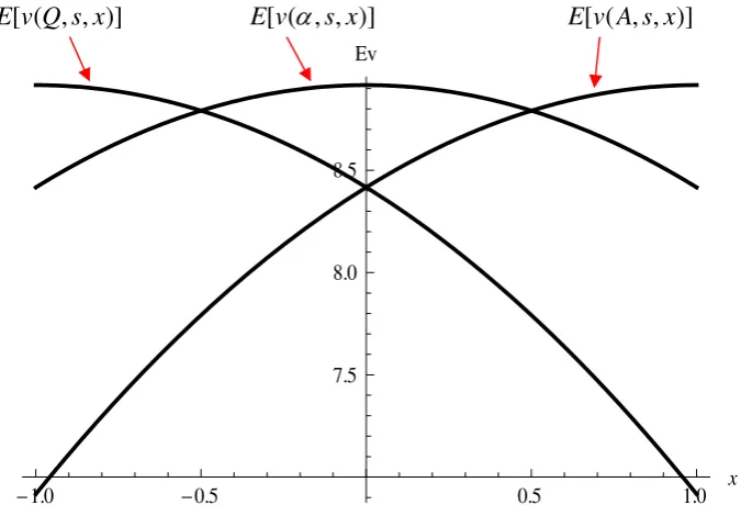
Hence, the political expected utilities are computed as
E[v(Q; s; x)] =
Z 1
0
v(Q; s; x)ds =K 1
12 6x
2
+ 12x+ 19
E[v(A; s; x)] =
Z 1
0
v(A; s; x)ds =K 1
12 6x
2
12x+ 19 :
In the case of full information equivalence,
E[v( (s); s; x)] =
Z 1=2
0
v(Q; s; x)ds+
Z 1
1=2
v(A; s; x)ds=K 1
12 6x
2
+ 13 :
See Figure 1 for these political expected utilities.
Existence of stable equilibrium:
The part of the Theorem concerning national elections follows from Feddersen and Pesendorfer (1997) and the argument that a second stage equilibrium exists if a second stage N-equilibrium exists for each N. The part of the proof concerning local elections proceeds as follows. First, we …nd a candidate symmetric allocation. Then we prove that it is an equilibrium. Finally, we prove that it is stable.
We will guess that district 1 always votes unanimously for Q, district 3 always votes unanimously for A, and district 2 satis…es full information equivalence, so the state-dependent outcome in district 2 is the same as the outcome with no uncertainty. For notational purposes, de…ne that outcome to be (s).
U1x = u1 +E[v(Q; s; x)]
U2x = u2 +E[v( (s); s; x)]
U3x = u3 +E[v(A; s; x)]:
Given an axisymmetric distribution (13), we de…ne the potential equilibrium value 2[0;1
2]to be the minimal value of such that the marginal consumer is indi¤erent
between districts 1 and 2:12
u1( ) +
Z 1
0
v(Q; s; F 1
( ))dG(s) = u2( ) +
Z 1
0
v( (s); s; F 1
( ))dG(s):
Next, we show that this is in fact an equilibrium. To accomplish this, we must simply consider the decision of one individual at this allocation. No individual can unilaterally a¤ect the economic allocation in any district, no matter their action.
To show that this is a second stage equilibrium in the political sector, we must show that it is a second stageN-equilibrium forN tending to in…nity, where we draw agents randomly in their respective districts. For the polarized districts, this is easy, since the strategy pro…le that has everyone voting for example for Q in district 1 means that nobody is ever pivotal. As argued in section 3, this Nash equilibrium strategy pro…le is the only one that is weakly undominated. The harder case is district 2, the middle district. Since nothing is learned from conditioning on being pivotal, players rely only on their private signals, as in Feddersen and Pesendorfer (1997, Example 2). Hence a second stage N-equilibrium for district 2 exists and satis…es full information equivalence. So a second stage equilibrium exists.
So now it is simply a matter of showing that the agents we have assigned to each district are at least as happy with the outcomes in that district as they would be in any other. By symmetry, if the argument works for one side of the distribution, it works for the other. So we focus on the left side. Notice that since v(s; x) is increasing in s and x,v( (s); s; x) v(Q; s; x) is non-decreasing inx for eachs.
u1( ) u2( )
=
Z 1
0
[v( (s); s; F 1
( )) v(Q; s; F 1
( ))]dG(s):
So forx F 1( ),
u1( ) u2( )
Z 1
0
[v( (s); s; x) v(Q; s; x)]dG(s)
and thus Ux
1 U2x. A similar argument works forx F 1
( ), implying Ux
2 U1x.
A symmetric argument holds for the boundary between districts 2 and 3. Notice that this argument also holds if = 1
2, noting that (s) is replaced by A in the
expressions above.
is easier, and is the one we will use, the issue is that their framework is set up for homogeneous consumers. Obviously, we have heterogeneous consumers/voters. So in order to apply the result, we formulate an arti…cial model that gives all consumers in a district the utility of the consumer at the margin or boundary for that district. Then this arti…cial model …ts into the framework of Tabuchi and Zeng (2004).
De…ne
U1( 1) = u1( 1) +
Z 1
0
v(Q; s; F 1( 1))dG(s) (15)
U2( 2) = u2( 2) +
Z 1
0
v( (s); s; F 1
(1 2
2
2 ))dG(s)
= u2( 2) +
Z 1
0
v( (s); s; F 1(1 2 +
2
2))dG(s)
U3( 3) = u3( 3) +
Z 1
0
v(A; s; F 1
(1 3))dG(s);
where
1+ 2+ 3 = 1: (16)
The remainder of the proof consists of 3 steps. First, apply Tabuchi and Zeng (2004, Theorem 2) to the system de…ned by (15) and (16) to obtain generic existence of a stable equilibrium for this system. Actually, we must delve into the proof of Lemma C1 of that paper, p. 659, as it is not immediately clear that Theorem 2 of that paper applies to a standard New Economic Geography model, such as our economic sector. (Recall that only the economic sector matters for stability, due to our de…nition of stability.) As it turns out, the Theorem does apply. From the discussion just below equation (11), it follows that the indirect utility of a nonempty region is higher than that of an empty region. Moreover, from standard calculations for the New Economic Geography model, we know that the derivative of indirect utility as a function of cannot be zero. Thus, conditions (i) and (ii) of Tabuchi and Zeng (2004, pp. 658-659) arealwaysmet (not just generically), so a stable equilibrium exists.
Second, we claim that there is no asymmetric equilibrium of the system (15) and (16), so the stable equilibrium must be symmetric, namely 1 = 3. This holds
contradiction.
Third, we claim that any stable equilibrium of the system (15) is also a stable equilibrium for the original system in the sense of equation (12). It is an equilibrium of the original system because the utilities of the consumers at the boundaries between districts are equated. Stability holds because the derivatives of the two systems, evaluated at equilibrium populations, are the same. This is easily veri…ed for each part of the left hand side of inequality (12), where each part is evaluated at the boundary (in consumers/voters) between districts.
Characterization of Stable Equilibria:
Due to symmetry, the necessary condition for interior equilibrium is given by
U( ) U2x U
x
1jx=1 = 0:
(i) Full agglomeration in district 2 ( = 0)
Suppose all individuals are agglomerated at district 2. Plugging = 0 into (10), we havew = 1=", and thus,
U(0) = L
"c 1 " 1
1 "2("" 11) 1
2:
Full agglomeration at district 2 is a stable equilibrium if and only if U(0) 0. Solving U(0) = 0, we get the agglomeration sustain point:
A " 1 1 2 "c L 1 " 1
#"(" 1) 2" 1
2(0;1) if 1> 1
2 "c L 1 " 1 :
Hence, full agglomeration emerges if the …xed labor requirement is su¢ciently small relative to the mass of workers (c < c0 2" 1L
") and the transportation cost is large enough ( A).
(ii) Strati…ed equilibrium with district 2 empty ( = 1=2)
This is an equilibrium with a symmetric population distribution in districts 1 and
3. Substituting = 1=2 into (10) yields w = 1+2
1 "
. Strati…ed equilibrium with district 2 empty exists if
U(1=2) = L
"c 1
" 1 " 2" 1 "(" 1) 2
1 +
1
" 1 +
2
1 " 1#
Solving for Lc yields
L
c h1( ; "); (17)
where
h1( ; ") =
"
2" 1 1+ 2
1
" 1 "2("" 11) 2
1+
1 "
" 1:
This equilibrium is stable if
d
d U3 U1 =1=2
<0:
Solving for L
c by using (11) for this speci…c symmetric distribution yields
L
c < h2( ; "); (18)
where
h2( ; ") =
2"
1 +
(" 1) (2"+ 1) (2" 1) (1 )
" 1
:
Therefore, there exists a stable strati…ed equilibrium with district 2 empty if
h1( ; ")
L
c < h2( ; "): (19)
It can be shown that
lim
"!1; !0h1( ; ")<0 and "!1lim; !0h2( ; ") =1.
By continuity, (19) holds for any given L and c if " is su¢ciently large and is su¢ciently small. Hence, the strati…ed equilibrium emerges and is stable if the goods are complementary (" "0) and the transportation cost is large enough (
B).
(iii) Partial agglomeration ( 2(0;1=2))
When is su¢ciently large, full agglomeration in district 2 is not an equilibrium because lim !1 U(0) = 1=2<0. Similarly, full agglomeration in district 1 or 3 is
not an equilibrium.
When is su¢ciently large, the strati…ed equilibrium with district 2 empty does not exist because lim !1 U(1=2) = 1=2>0. Similarly, there is no equilibrium with
district 1 or 3 empty.
Figure 1: Political expected utilities with K=10
)] , , ( [v Q s x
E E[v(
,s,x)] E[v(A,s,x)]-1.0 -0.5 0.5 1.0 x
7.5 8.0 8.5
Ev
Figure 2: Equilibrium distributions when
5andL/c100Dotted arrow is L1, solid arrow is L2 and dashed arrow is L3
B
A0.0 0.2 0.4 0.6 0.8 1.0 f
20 40 60 80 100
[image:32.595.84.448.485.752.2]