Munich Personal RePEc Archive
Estimating the value of additional wind
and transmission capacity in the rocky
mountain west
Godby, Robert and Torell, Greg and Coupal, Roger
University of Wyoming, Laramie, USA.
16 January 2013
Estimating the Value of Additional Wind and Transmission Capacity in the Rocky Mountain West.
January 2013
Robert Godbya, Greg Torella and Roger Coupalb
Contact and correspondence, please email: rgodby@uwyo.edu.
Mailing Address: Robert Godby
Department of Economics and Finance University of Wyoming
Laramie, WY 82070 USA
307-766-3843
Comments welcome. All errors remain the authors’ alone. This work has been supported through a grant from the University of Wyoming School of Energy Resources, Center for Energy Economics and Public Policy.
a.
Department of Economics and Finance, University of Wyoming
Abstract
The expansion of wind-generation in the United States poses significant challenges
to policy-makers, particularly because wind’s intermittency and unpredictability can exacerbate problems of congestion on a transmission constrained grid. Understanding
these issues is necessary if optimal development of wind energy and transmission is to
occur. This paper applies a model that integrates the special concerns of electricity
generation to empirically consider the challenges of developing wind resources in the
Rocky Mountain region of the United States. Given the lack the high frequency data needed
to address the special problems of intermittency and congestion, our solution is to create a
dispatch model of the region and to use simulations to generate the necessary data, then
use this data to understand the development patterns that have occurred as wind
resources have been developed.
Our results indicate that the price effects caused by changes in power output at
intermittent sources are strongly dependent on supply conditions and the presence of
market distortions caused by transmission constraints. Peculiarities inherent in electric
grid operation can cause system responses that are not always intuitive. The distribution
of the rents accruing to wind generation, particularly in unexpectedly windy periods are
strongly dependent on the allocation of transmission rights when congestion occurs, which
impacts potential returns to developing wind resources. Incidents of congestion depend on
the pace of development of wind and transmission capacity. Not accounting for such
distortions may cause new development to worsen market outcomes if mistaken estimates
Introduction:
The expansion of wind-generation in the United States poses significant challenges
to policy-makers. Of primary concern is how to incorporate wind and other renewable
resources into the existing electricity-grid while maintaining power supply at low cost and
high reliability. On the supply side, adding generation with the unique characteristics of
wind and solar power to the grid presents significant reliability and cost challenges.
Electricity cannot easily be stored and the intermittency and unpredictability of these
sources can make scheduling electricity in a reliable but efficient way difficult.
Transmission capacity and network congestion also complicate these efforts (see Green
and Vasilakos, 2008, DOE, 2009 and NREL, 2010 as examples). On the demand side,
electricity demand is unresponsive to cost change, lacking both the information to react to
cost conditions and changes, and the short-run flexibility to meaningfully change an
inelastic demand. Given supply must always equal demand on an electricity system and
that demand will not respond to changes in the availability of wind energy, sudden
increases in the wind energy can cause significant economic changes as well as operational
problems on the electricity-grid. This paper attempts to illuminate these problems and
their interrelationship with a simulated model of the Rocky Mountain area power grid.
Among renewable sources, wind power poses the most serious challenge to
electricity network planners and regulators due to the intermittency of the resource. While
backstop sources can be added to the grid for use when wind or other renewable resource
availability is low, these large fixed capital investments are costly and their use as a
backstop ensures lower capital return and higher system costs than when the same
generation sources, along with the spatial location of wind generating sources could reduce
the potential intermittency of total generation, and reduce the fixed costs of backstop
sources necessary to ensure system reliability. Location of wind resources, however, often
requires transmission capacity to deliver power to market when it is available. Since
intermittency exists, the coordination of wind generation to total demand on a fixed
transmission system can be difficult and result in problems of congestion. Congestion may
occur due to demand spikes in one portion of the grid requiring delivery of additional
power using the transmission network, or from unexpected increases in renewable
generation, which strains the transmission system capacity to deliver this low-cost power
to load. When such congestion events occur, local rents can be created for generators in
areas where congestion constrains deliverable energy as the value of energy on the
downstream side of any constraint rises relative to uncongested conditions. Significant
rents may not only be created for generators within the areas affected by constrained
delivery capacity, but they may also be created for the holders of transmission rights able
to deliver to such areas. Understanding the stochastic nature of wind energy and the
grid-cost dynamics of this resource also requires an understanding of system-wide transmission
outcomes and the associated economic rents generated by wind installations. This requires
a modeling framework that mimics the special nature of electricity markets, the problems
posed by inelastic demand and lack of inventory or storage.
A challenge to the empirical study of renewable energy integration is a lack of data,
specifically high frequency (hourly or higher frequency) wholesale electricity price data
that describe market outcomes. Spot prices for electricity in specific regions are not
often reported as an index of average prices representing lower frequency intervals. The
nature of demand, renewable generation changes, as well as transmission congestion on an
electricity system is that they are intermittent. Congestion can occur in several hours in a
day and then disappear for several hours or days depending on network conditions. In
order to understand the nature of intermittent sources, congestion rents and price impacts,
high frequency (hourly or better) data is necessary. To overcome this challenge simulation
methods are used here to model market prices and estimate potential congestion effects
using available hourly demand and transmission data.
This paper informs policy with a simulation model of an electrical grid that
incorporates the stochastic nature of wind resources to explore the dynamics of system
costs. Results are presented for a model of the Rocky Mountain Power Area (RMPA), an
area that encompasses most of the state of Wyoming, all of the state of Colorado and small
areas of some adjacent states in the western United States. This area is of particular
interest to consider the potential economic issues of integrating wind resources for several
reasons. First, areas of the RMPA have some of the best potential for wind power
development in the United States. Second, this area experienced a significant build-out of
wind development and other transmission sources over a short period of time while
transmission capacity and other grid conditions remained relatively unchanged. Third,
because of its relative size compared to other control regions in the United States, the
Rocky Mountain Area is more easily modeled than other larger regions. These
characteristics allow a study of the area to inform and quantify the congestion costs of
The simulation model used to model the RMPA minimizes estimated system costs
while meeting transmission constraints and power demand on an hourly basis using actual
data from the years 2008 to 2010 to simulate hourly generation, price outcomes and
network congestion conditions. Two types of generation sources are used with unique cost
and capacity characteristics reflecting actual field relationships: (i) traditional and
non-intermittent sources including fossil-fuel thermal-generating (coal and natural gas) units
and hydro-electric generation, historically developed to exploit the existing natural
resources in the study area, (ii) wind generators whose cost and capacity conditions reflect
the local stochastic climate conditions. Using the model output, hourly estimates are
computed of efficient power market prices. When transmission congestion occurs these
are used to estimate congestion rents that occur over a three-year period. These rents
form an estimate of the social benefits of reducing grid congestion through possible
transmission system expansion if additional renewable resources are to be added to the
electrical grid. Congestion rents are also related to wind outcomes to describe the
potential impediments to wind development caused by grid conditions, and which may
explain observed patterns of actual development while predicting future challenges to
additional large scale wind development.
Such information is critically important to policy-makers, especially if there is to
continue to be public-sector involvement in fostering conditions for renewable energy
development and integration, and in identifying where such public involvement would be
most beneficial. For example, the state of Wyoming’s wind generation capacity in the RMPA
increased by a factor of eight from 2007 to 2010, jumping from 143.4 MW of potential capacity in 2007
the state is still largely untapped. In Colorado during the period from 2008-2010 only 236 MW of wind
capacity was built (increasing from 1063 MW to 1299 MW), but since then it has increased by over
500MW, with an additional 16,602 MW planned.1 This shift in development has had significant
economic impact to both states. According to officials in Wyoming and Colorado, the greatest
impediment to additional development in both states is the lack of transmission capacity out of the RMPA
necessary as the combined planned development in both states is twice their peak demand levels.
Transmission congestion between Wyoming and Colorado within the RMPA, however, has also been
cited as the reason why development in Colorado continues to occur while in Wyoming development has
not since 2010, despite the fact that wind resources in Wyoming are considered to be better than those in
Colorado. To overcome this hurdle the state of Wyoming embarked on financing a $200 million
transmission capacity enhancement between the two states. Some might wonder why, if such
development were so valuable, is state involvement necessary when in the past private entities have
developed such transmission capacity? This question is even more relevant given several multi-billion
dollar fully private projects are underway to expand potential transmission capacity out of Wyoming to
locations over five times more distant. This puzzle regarding why there is less private interest in making
smaller investments to improve transmission infrastructure to nearby markets than to embark on very
expensive projects to serve more distant ones is also an example of questions that might be answered
using such a model.
The paper proceeds as follows: a description of the generation, transmission and
institutional context present in the western United States and Canada is described and the
study region is introduced. A simple theoretical model is then presented to describe the
electricity dispatch problem. A solution to this system provides a simulation framework
that can then be parameterized for the study region. A simple parameterization of the
Rocky Mountain Power Area is outlined in a static context to demonstrate how problems of
1
intermittency and transmission capacity can impact energy cost outcomes. Solutions are
then presented from the hourly simulation model. These results are used to estimate
market price outcomes and to describe how the rents created by wind generation can vary
with the stochastic nature of wind as an energy resource, as well as the stochastic nature of
electricity demand, and how these rents could be influenced by the existence of specific
transmission constraints. Conclusions are then presented based on the findings described.
Electricity Generation in the Rocky Mountain Power Area.
The North American electricity-grid in Canada and the United States actually
consists of three separate and isolated grids, the eastern and western interconnects, and
the ERCOT (Texas) interconnect. These span the United States and Canada and include a
small portion of Mexico. The North American Electric Reliability Corporation (NERC)
administrates standards to ensure the coordination between interconnections and the reliability of
the grid within each. Electricity generation and supply in the western United States and
Canada is administrated by the Western Electricity Coordinating Council (WECC), which
further sub-divides this grid into four reporting areas, one of which is the Rocky Mountain Power
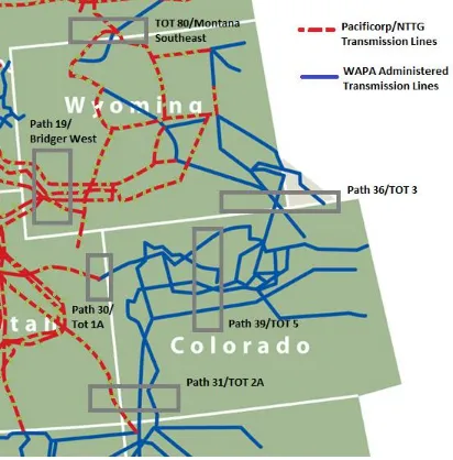
Area (RMPA). The geographic boundaries of the WECC administrated western interconnection
and the RMPA are shown in Figure 1.
The Rocky Mountain Power Area (RMPA) provides power to over 5.5 million people
within all or parts of five US states: the entire state of Colorado, eastern and central
Wyoming, portions of western South Dakota and Nebraska, and a small area in the extreme
northwest corner of New Mexico. Figure 2 presents the RMPA transmission network.
and several much smaller municipal utilities and rural electric associations.2 These entities
engage in generation and/or purchase wholesale power through bilateral trades with
suppliers of electricity. Generation facilities are located throughout the RMPA, however
renewable sources; specifically wind generators are primarily located in central Wyoming
and northeastern Colorado. Transmission access to deliver generated power to RMPA
load-centers may be scheduled through utilities’ own transmission facilities or through two transmission networks. A simplified schematic of the RMPA transmission networks is
shown in Figure 2. The simulations presented here assume an efficient market outcome
and ignore any price distortions that may actually occur due to these institutional realities.3
Modeling Framework
To model and evaluate the wind energy generation, transmission and policy issues
within the RMPA, a DC load-flow modeling framework is used to model hourly generation
price and generation outcomes as an approximation to the actual AC system.4 The modeling
framework follows the nodal pricing model outlined by Green (2007) and formalizes the
choice of generation sources used (referred to as “dispatch”) to serve a given demand or “load” subject to the technical constraints of the electric-power network. The general
2
Three investor owned utilities serve the RMPA: Rocky Mountain Power (a subsidiary of PacifiCorp) in central and southeast Wyoming, Black Hills Power serving eastern Wyoming, parts of Nebraska, South Dakota and Colorado, and the Public Service Company of Colorado (Xcel Energy) serving central Colorado including the Denver region. There are also 29 municipal utilities in Colorado and three in Wyoming, 15 rural electrical cooperatives in the
RMPA area of Wyoming and 26 in Colorado (Navigant, 2010 and Wyoming Office of Consumer Advocate website. 3
The RMPA does not utilize an organized power market. Some authors have noted that the existence of multiple power providing agencies using bilateral power contracts could result in a less than efficient outcome (Beck, 2009). 4
modeling problem assumes that the system minimizes generation cost.5 The relevant cost
of electricity generation is the variable cost of producing each unit of output measured in
megawatts (MW), and ignores fixed costs of production.6 Total costs are minimized
relative to the technical constraints of the system; specifically that generation (supply
including line losses) and demand are always balanced, that total generation cannot
exceed generation capacity plus system net imports, and that transmission flows do not
exceed capacity constraints. Generation and demand occurs at all nodes in the transmission
system, and transmission systems allow power flows between nodes. The general problem
to be solved on an hourly basis can be described as
s.t.
(Generation capacity constraint)
(energy balance constraint)
(transmission line flow constraint)
(individual generator production constraints)
5
Unlike Green, 2007 and other papers, due to the hourly frequency of the simulation we do not maximize net benefit and take reported demand within the region as given. This makes the demand modeled perfectly inelastic. 6
This is consistent with the theory of profit maximization in the short run. Variable costs include include fuel and production input costs, operation and maintenance costs that vary with the quantity of output. See standard
hich gives the associated Lagrangian:
where dk is the net demand at node k, wj,k is the power generated at generator j in node k
where k = 1, 2 and z is the flow of power along the transmission line connecting nodes k = 1,
2 given the RMPA can be modeled as a 2-node network. Transmission lines each have a
fixed capacity of zmax and flow on the transmission line is defined as the difference between
demand and supply in each node. Total line losses in the system are l. NI defines
exogenous system net imports of generated power from outside the RMPA and can be
positive or negative. Generators cannot exceed their capacity.7 e is the Lagrangian
multiplier associated with the energy balance constraint that demand plus line losses must
equal generated power and any net imports, and TS is the multiplier associated with the
transmission line i capacity constraint. The first order conditions of equation (6) with
respect to optimal choice of generator choice and output (dispatch) and taking constraints
and net imports as given, the optimal price at each node in a 2-node system can be found:
.8
The multiplier on the energy balance constraint is equal to the marginal cost of generation
at the swing bus in the absence of line losses, where the swing bus is the node defined to
contain the last unit of generation called upon in an optimal (cost minimizing) dispatch.
Due to the existence of line losses, more or less than one unit of generation can be required
to create an additional unit of power. Increasing line losses would require a greater than
7
We assume that the all generators face no constraints regarding the ability to supply less than full capacity. 8
one unit increase in generation to create one more unit of power at the load, but if due to
line constraints, the optimal configuration of generators across the network changed to
accommodate the extra power, it can also be the case that line losses will fall, resulting in
less than one unit of additional generated power being necessary to create one additional
unit of power delivered to final demand.9
The second term in this equation shows how line constraints affect marginal costs at
each node. When the transmission constraint is non-binding, TS =0 and the price in the two
nodes is equal. Consider a cost minimizing outcome in a 2-node system and suppose that in
the optimal solution the combined load of both nodes is just met by the combined
generation in each node, with the last unit of generation dispatched in the upstream node.
If a single transmission line operates between the nodes and is just at maximum capacity
(in which case the transmission line is said to be “just congested”), any additional unit of demand added at the downstream node will require the additional generation to take place
in that node and the transmission constraint will be binding. The price in node 2 will differ
from that in node 1, with the price in node 1 equal to the price of the marginal unit of
generation there, and the price in node 2 equal to the price of the marginal generation at
the new source of generation. The value of TS would then become the difference between
the marginal costs of the last generators dispatched in each node. The second multiplier in
(2) is then the difference between the cost of power on the network at the swing bus and
the marginal cost at a node with a line constraint.
9
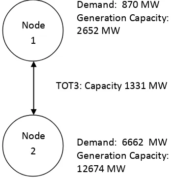
To implement the cost minimization model summarized in a simulation context the
transmission network described in Figure 2 can be reduced to a 2-node network. This
methodology is consistent with published results in other power studies including DOE
(2009).10 Node 1 comprises all areas in the RMPA north of Wyoming border and Node 2 all
areas south (the state of Colorado). Power can flow between Wyoming and Colorado only
using a transmission pathway referred to in the industry as Path 36/TOT3. Figure 3
presents the simplified nodal network, identifying average demands, generation capacities
transmission capacities used in the simulations. WECC Path Data is used to define NI for
the pathways shown in Figure 2 leading out of the RMPA and it is subtracted from total
nodal loads consistent with Equation 3.11
Implementing the simulation model also required identifying RMPA generation
potential. Generator capacities by site were defined using EIA form 860 data for over 360
individual sources. Fuel sources within the RMPA include coal, natural gas, hydropower,
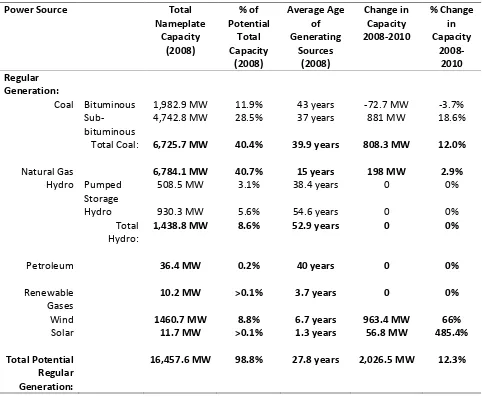
diesel fuel, wind, solar power, and renewable gases. Table 1 describes generation capacity
by fuel type or power source within the RMPA at the end of 2008 and changes in capacity
through 2010. The growth of wind resources is clear – wind potential grows 66% from 8.8% to 13.1% of total generation capacity from 2008-2010. The only other major source
of growth in generation capacity over this time period was in coal generation, which
increased by 12%, increasing coal’s share of total potential generation from 40.4% to
40.8%. The growth in wind capacity was from 2008-2010 is even more dramatic when
10
WECC (2012) and DOE (2009) model the RMPA as a three-node system splitting Colorado into eastern and western nodes. Both studies find no congestion on this pathway, these two areas are modeled as a single node. 11
considered by Node. Wind generation capacity in Wyoming (Node 1) increases by from
143 MW to 1130 MW of potential power, while Colorado Wind potential increases by 229
MW to 1292.1 MW over the same period.
To estimate an efficient dispatch outcome that minimizes total generation costs as
previously outlined, individual generator costs must be identified or estimated. Since such
costs are proprietary, little of such data exists publicly. Many cost estimates exist in the
economic and policy literature, but these studies most often consider the capital costs
necessary to create new generating capacity, which are inappropriate for use in the
theoretic model described.12 Marginal generator costs are instead estimated using
published production engineering estimates of their determinants, plant characteristics
from EIA Form 860 data, published fuel and transport costs, and transmission costs based
on the location of generators. The methodology used to estimate these costs
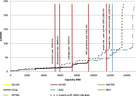
deterministically is detailed in the Appendix.13 Figure 4 shows the modeled efficient
dispatch “merit order” or supply curve for the entire RMPA assuming no transmission
congestion occurs between nodes using summer 2008 reported peak capacities, and
estimated marginal costs by generator expressed in 2008 dollars. Maximum generator
capacities are shown by fuel type, which determines plant marginal costs. Lowest cost
generators in the dispatch order are renewable sources: solar, wind and hydro as their fuel
is effectively free and the only costs faced are those operations and maintenance costs that
12
Studies often consider “levelized” costs - all capital and fixed costs, financing costs and forecasted operating costs averaged over the projected lifetime of the plant. Others cite the “overnight cost” of a plant - the total cost to construct a plant if it were built in one night. Neither of these costs is appropriate to model dispatch. In the long run, fixed costs are covered by the economic rents created by inframarginal units of generation. See Stoft (2002). 13
increase with output. Solar and wind power have significant intermittency and the
potential effect on the estimated supply curve of wind intermittency in particular is shown
by the broken line which reduces wind capacity to 12% of potential capacity as used by
NERC to estimate system reliability. If renewables were to provide 100% potential power,
this would shift the supply curve by about 1300MW to the right, and this could significantly
alter power market conditions.
To illustrate the hourly power dispatch market outcomes the simulation model
computes (without the complication of transmission congestion) and how they vary with
the potential intermittency of wind generation, Figure 4 shows summary measures of
actual 2008 hourly RMPA load data reported, along with NERC’s summer 2008 forecast peak load (NERC, 2008). The efficient market price and quantity of electricity is shown for
the minimum, maximum (average and forecast), average, 5% and 95% load levels by the
intersection of the supply curve and these demand levels, conditional on wind output.14
The estimated equilibrium wholesale price of electricity in the market would have ranged
from a minimum cost of $15.38/MWh to a maximum of $77.02 ($77.10 at the forecast
peak), would have ranged from $15.50 to $39.63 in ninety percent of the hours in 2008,
and averaged $29.38 over 2008 assuming that the wind output was 12% of potential
capacity. This is a very conservative worst-case scenario but in any hour the shift of the
supply curve could be more dramatic than presented as occasionally almost no wind power
is present on the grid. At maximum wind potential, the efficient market prices at the given
loads would have ranged from $12.24 to $45.90/MWh ($59.76 at the forecast maximum),
14
would have ranged from $12.93 to $39.21 in ninety percent of the hours, and averaged
$15.50 over the year. These results, however, assume no congestion occurs on the
transmission pathway between Nodes 1 and 2. If congestion were to occur, the RMPA
market would separate into two distinct markets, and a dispatch solution similar to that in
shown in Figure 4 would be computed in each. Power would flow along the transmission
line from the node with the lower price to that with the higher price. The supply curve in
the higher priced node would be composed of the residual supply curve from Node 1 up to
the capacity of the transmission line and the generator marginal costs located in that node.
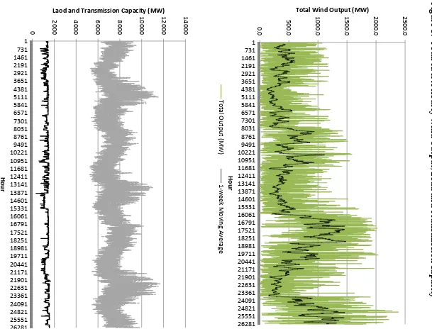
Hourly simulation solutions solve the simple problem illustrated in Figure 4 using
estimated generator marginal costs, generator capacities for traditional generators,
simulated wind capacities using weather data at each wind farm in the RMPA, actual RMPA
demand data and actual transmission constraints hourly from 2008 to 2010. The hourly
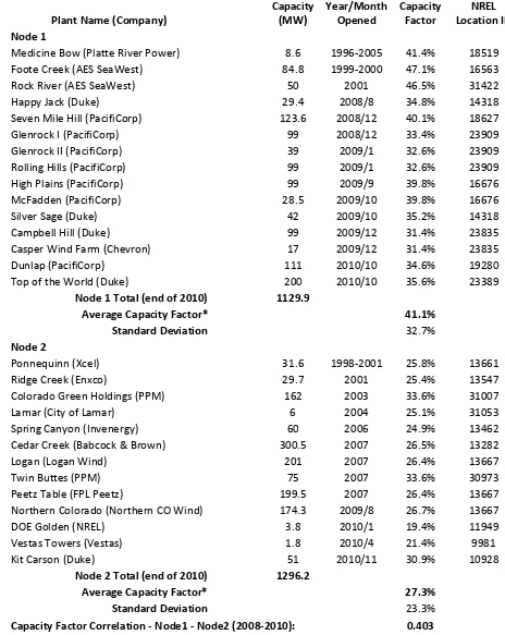
wind outcomes used in the simulations are summarized in Figure 5 and Tables 2 and 3.
The RMPA included 28 windfarms in 21 separate locations during the 2008-2010 period.
As noted in Tables 1 and 2, wind capacity grew over the simulation period. Lacking data on
exact start-up dates for new expansions, a plant was assumed to come online in the first
hour of the month it began operation. To model the wind at each plant location, the
National Renewable Energy Laboratory (NREL) Western Wind Dataset was used.15 This
dataset models hourly wind patterns across the western United States based on 2004-2006
data over 32,403 actual and potential windfarm locations in the western United States. The
meteorological model also accounts for and simulates spatial and temporal correlations
across the region. Data from the nearest locations modeled by NREL to each of the RMPA
15
windfarms was used to simulate wind outcomes by farm.16 The summary data in Table 2
explains why wind resources are so valued, particularly in Wyoming. The average capacity
factor of all Wyoming sources in the simulation was 41.1% while in Colorado it was 27.3%.
Both wind areas have a strong seasonal component as well as a diurnal one, and both
experience stronger winds and higher capacity factors in winter than summer months.
Colorado wind tends to peak at night, while Wyoming wind often a peaks in late afternoon.
Hourly balancing area load-data from Federal Energy Regulatory Commission
(FERC) Form 714 was used to define nodal demands.17 Since balancing areas do not
correspond to the nodes defined in the simulations, it was assumed underlying demand is
similar on a per-person basis in each node, and annual county-level census data from
2008-2010 was used to define nodal demands as the population-weighted shares of the total
load. This leaves an asymmetric pair of markets with Node 2 accounting for approximately
88% of total demand over the three year period. Demand patterns on a daily basis reflect a
typical diurnal pattern, peaking in daylight hours, with clear shoulder periods in evening
and mornings, and minimum demand occurring overnight. Seasonal peaks occur in
mid-summer, with a secondary peak in mid-winter. The data may also contain an economic
cycle, with average load falling during the 2008-2009 national recession. Hourly demands
are treated as perfectly inelastic and exogenous in the simulation model, as almost all
16
Capacity factor refers to actual power produced relative to the potential generation, or "nameplate" capacity. 17
residential and commercial demand in the region does not have real-time metering, nor are
instantaneous spot prices posted or charged. The three year demand pattern is shown in
Figure 5 and described in Table 3.
The ability of the grid to maintain low generation costs depends on transmission
constraints present on the grid. Actual hourly transmission limits for Path 36/TOT3 in
2008-2010 are also described in Figure 5 and Table 3. While the nominal capacity of this
link is 1605MW, its maximum rating in any given hour can vary depending on load and
generation conditions, temperature and weather, maintenance operations and
configuration changes, other transmission line conditions in the RMPA and reliability
considerations.18 For these reasons the average capacity over the simulation period was
1331 MW with a standard deviation of 173 MW. Transmission rights across this link are
determined by the ownership of the lines, which are both privately and publicly owned. As
of 2008, 71.4% of the capacity was owned by a consortium of utilities and agencies
involved in the Missouri Basin Power Project and owners of the Laramie River Generating
station in Wheatland, Wyoming, which can produce up to 1140 MW of power for the RMPA.
The remaining Path 36/TOT3 capacity is held by Xcel Energy (3.7%) and the federally
owned Western Area Power Administration (24.9%), which markets transmission rights
on its share of the link.
Results:
Electricity price outcomes are solved using the dispatch model and incorporating
actual RMPA demand (load) and transmission constraints, estimated generation costs,
18
wind conditions over the 26,304 hours simulating Jan 1, 2008 at 12:00 am to December 31,
2010 at 11:00 pm. A simulated unconstrained transmission solution in which no
transmission capacity was imposed between Nodes 1 and 2 was also computed using GAMS
to determine the impact of transmission constraints on the system. Results were also used
to consider the effects of wind intermittency and increased capacity on power prices and
transmission congestion, and to construct an estimate of congestion rents created by
inadequate transmission capacity between the two nodal markets. A summary of the
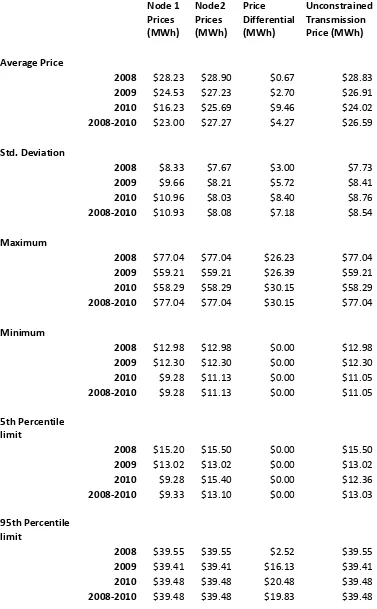
computed market price outcomes is presented in Table 4.
Price results indicate the effects of congestion on the grid. When the transmission
constraint is not binding price differentials disappear between Nodes 1 and 2. Comparison
of the efficient results to the results using the actual Path 36/TOT3 transmission limits
shows the constraint causes average prices in Node 1 to fall and Node 2 to rise relative to
the unconstrained case, as expected if power flows from north to south along the
transmission link. The impact of the constraint appears to increase over time as the
average price differential increases in each year, as does the standard deviation of prices in
Node 1 and for the price differential. Node 2 prices fall on average throughout the
simulation. Despite the fact that, all else equal, congestion should raise price in the
downstream node relative to the unconstrained outcome, the increase in the amount of
cheaper wind energy available in Node 1 over the simulation period both creates
transmission congestion which has the effect of raising Node 2 prices, and reduces the cost
of power exported from Node 1, potentially reducing costs in Node 2. In the unconstrained
transmission simulation the first effect is clear as the availability of increased low-cost
The change in congestion over time can also be seen by comparing annual price
differential outcomes. Figure 6 shows the duration of price differentials expressed as a
percentage of the total hours in each year of the simulation. Price differentials of a penny
or more between the nodal markets occur in only 7.2% of the hours in 2008, but this rises
to 20.5% of hours in 2009 and 69.3% in 2010. Additionally the maximum price differential
increases from $26.23 in 2008 to $30.15 in 2010, while average price differentials increase
from $0.67 to $9.46 in the same simulated period. While the incidence of congestion will
always occur more often when transmission capacity is reduced, as growth in wind
capacity occur ed in Node 1 the transmission capacity constraint appears binding in
significantly more hours regardless of the constraint level.
To quantify this impact a Tobit regression was run to determine the relationships
between demand, transmission capacity and the level of wind capacity available upstream
and downstream of the transmission constraint. These results are shown in Table 5. All
else equal, one would expect that growth in demand, which is always distributed in our
model proportionate to population in each node to reduce congestion as it allows the
upstream node a greater ability to absorb available power, leaving less for export. A
tightened transmission constraint will increase congestion. One would also expect that
since wind is unpredictable but nearly free when available, greater wind output in Node 1
would increase congestion by making more cheap power available for export to Node 2.
Increased wind in Node 2, however, would lessen the demand for Node 1 power as efficient
dispatch would use this energy first given it is cheaper than any exported power from Node
1 (it incurs no transmission costs since it is located in Node 2 and generation costs at each
results suggest the marginal effects of transmission constraints and wind output in Node 1
are an order of magnitude greater than demand changes or wind output changes in Node 2
suggesting these are the two primary determinants of transmission congestion price
differentials. On average, throughout the three year period, a 100 MW increase in
transmission capacity would reduce the price differentials by $3.75 while an increase of
100 MW of wind output in Node 1 (equivalent to approximately 243 MW of new capacity
given the average capacity factor of Node 1 wind-farms) would increase the average price
differential by $4.26.
To quantify the cost of increased congestion caused by additional wind capacity and
inadequate transmission capacity, congestion rents were also determined. These rents
were computed as the value of the exported flows from Node 1 to Node 2 given the price
differential in that hour. These form our estimate of the potential benefit of additional
transmission capacity being under efficient market conditions.19 To determine the amount
of capacity necessary to avoid these rents, simulations were also run increasing the
available transmission capacity in each hour by 100 MW increments up to 1000 MW.
Table 6 describes the congestion rents that were estimated to occur and the estimated
avoided rents of each additional 100 MW increment of transmission capacity. Results show
the increase in congestion rents accruing to transmission rights holders as predicted
congestion increased over time. Again, these appear to have been driven by the additional
generation capacity installed on the grid, particularly wind.20 The estimated value of total
19
Actual benefits in the RMPA are potentially higher given the fact that the wholesale market is not organized as a competitive auction but instead relies on bilateral agreements between utility providers and power generators. 20
rents accrued over the three simulated years was over $141 million. As shown in Table 6, a
relatively small addition of transmission capacity could have significantly reduced total
congestion rents in any year, with the first 100 MW potentially avoiding over 29% of the
total rents generated, and over half of the total rents generated in the years 2008 and 2009
respectively. In the first two years of the simulation an additional 500 and 700 MW of
capacity would have eliminated all congestion rents, while a 1000 MW increase would have
been necessary to nearly eliminate all rents in 2010.
Analysis of the distribution of estimated rents and how they change reveals how the
price and quantity changes in the market affect generator’s revenues, especially in the
presence of transmission congestion. Given the ownership of transmission rights over the
Path 36/TOT3 link, a single consortium of companies involved in the Missouri Basin Power
controlling one coal-generating station (the Laramie River Station) could earn an estimated
$101 million share of the rents generated under current market conditions.21 Only just
over $35 million could be earned from users of the transmission rights marketed by the
Western Area Power Administration’s (WAPA) to other producers in Node 1.22 The largest
utility in Node 2, Xcel Energy would be estimated to receive a $5.2 million share of these
rents.
A further analysis of rents accruing to all producers in Nodes 1 and 2 is presented in
Table 7. The presence of congestion and the impacts this has on prices in each node are
21
Results suggest that the Laramie River Station would only earn $87.6 million from rents due to exports to Node 2. The efficient dispatch would allocate some of this plant’s production to Node 1, leaving it unable to use its entire transmission rights allocation. If the plant could sell its excess transmission rights to other firms in Node 1 it could potentially capture the rents available, thus the actual rents to accruing to the consortium would likely be between $87.6 million and $101 million.
22
clear from comparison of profits for generators in Nodes 1 and 2 under the simulations
using actual hourly transmission limits, and those that could occur if such constraints were
not present. In Node 1, 9% of potential profits are lost due to congestion and the resultant
lower prices in that node, costing almost $80 million over the three years of the simulation.
Node 2 producers reap the benefit of the higher prices the congestion causes, which causes
total profits to rise by over $88 million, or over 4% relative to outcomes had no
transmission congestion occurred over the three years.
Wind producers are even more affected than the general market in Node 1 by profit
losses due to congestion effects. Because of the cost-minimizing dispatch that is assumed
to occur in each node, wind power is almost always sold in the node it is produced. For
Node 1 producers, very seldom is there a surplus of power available for export after such
dispatch occurs thus they earn very little rents. As wind capacity increases in Node 1 this
pushes coal-fired generation up the supply curve and closer to the margin, and contrary to
what might be expected, this actually can benefit some coal-producers as it allows them to
export more of their power and in times of congestion this allows coal-fired producers to
earn most of the congestion rents available. The result is improved profitability for the
coal-generation sector over what it would have been without such rents.
Wind producers in Node 1 have the opposite experience, and as their power
production rises over time, which then causes more congestion on the grid, prices fall in
Node 1, lowering wind-producer’s profitability. In effect, windier conditions, causing greater wind production costs wind producers while benefiting coal producers. Wind
producers suffer almost 47% of the total profit loss experienced in the Node 1 due to
congestion effects. Most of the remainder of the profit loss in Node 1, particularly in the last
year of the simulation is experienced by hydro-electric producers.23 While some coal
plants can experience profit loss due to congestion-caused lower prices in Node 1, as a
sector, coal-generation in Node 1 becomes the primary export power source when
congestion occurs and actually experiences increased profits when congestion occurs. 24
Node 2 wind producers benefit from the congestion caused by abundant and low-cost
production in Node 1. Their profits over the entire simulation rise by 22% relative to
simulations without a transmission constraint, accounting for 44% of the total profit
increase in that node.
Discussion of Results
The impact of the additional wind output in our simulated RMPA markets is
dramatic when transmission congestion occurs. Congestion caused by additional wind
energy causes regional market prices to diverge, sometimes significantly on average from
those that would occur in uncongested circumstances. Price results presented in Table 4
for the RMPA simulations suggest the greatest impact to prices occurs in Node 1 where
prices fall due to the stranded wind power flooding the local nodal market and driving
wholesale prices downward. While it may seem initially counter-intuitive, additional wind
energy arriving on the grid is not necessarily a benefit to wind producers as the price
decreases caused in Node 1 by congestion can eliminate much of the additional profits the
23
Hydro electric generation accounts for 290.1 MW of potential power in Node 1 and collectively defines the next step on the supply curve above wind generators. Coal generators are collectively grouped in the next portion of the supply curve for Node 1, and the marginal generation type in most hours.
24
additional power might create. Further, traditional fossil-fuel power producers are
displaced in the dispatch queue by sudden and unpredicted increases in wind power.
While this could be expected to lower the profits and return to these capital assets if their
generated power were dispatched locally, both due to the lower prices congestion creates
and potentially reduced power output as more expensive coal-fired power becomes less
competitive, this need not happen. Our simulations show that if these plants have
transmission rights, exporting their power to neighbouring markets where prices due to
congestion become higher can allow them to offset such losses and actually benefit from
the presence of wind-generators. Overall then, the addition of unpredictable wind
resources in a transmission constrained area such as Wyoming can have the effect of
lowering returns to capital for wind producers in that area relative uncongested
conditions, while having an ambiguous effect on higher-cost traditional generators.25
Downstream of the congestion the effect is the opposite. Congestion has the effect of
driving a wedge between the efficient power price and transmission constrained outcomes,
raising profits over what they would have been without congestion. The effect to
consumers in the downstream market would likely be unambiguous; customers whose
utilities were forced to pay higher wholesale prices than would occur in the absence of
congestion would face higher prices.
The impact of congestion on power market outcomes also may not create price
incentives for the creation of additional transmission capacity. In the results presented, the
estimated additional capacity needed to avoid congestion is over 1000 MW by the end of
25
the simulation. While transmission expansion costs vary by location, the Wyoming
Infrastructure Authority estimates the cost of an 800-900 MW expansion of the Path
36/TOT3 line modeled to be less than $300 million.26 Simulated Node 1 price outcomes
and profit outcomes suggest that wind generators have little incentive to provide
additional transmission capacity to Node 2. Node 1 wind producers’ lost profits over the three year simulation total $37.3 million, suggesting the payoff time to such an investment
could be decades. Further, wind generators are owned by multiple firms suggesting that
coordination for such an investment could be difficult and free-riding incentives could
undermine any such effort. Increases in capacity would have no benefit and potentially
create losses for wind producers downstream of the congestion as it would eliminate most
of the congestion rents and price differentials occurring that drive their estimated excess
profits over unconstrained conditions. Ironically, increases in wind output seem to create
the greatest benefits in Node 1 to fossil-fuel generators with transmission rights to Node 2
thus they would have little incentive to invest in additional capacity. Third-party
transmission companies may also not be willing to invest in additional transmission
capacity for the same reasons - doing so would reduce the rents and potential profits of
building more lines.
Comparing the predicted simulation outcomes and implied incentives to actual
development in the RMPA suggests the results are consistent with the observed pattern of
development. Initially wind resources were exploited in Colorado nearest the major load
center in the area (the City of Denver). While Wyoming’s wind resources were known to be
superior in quality to those in Colorado they were initially developed slowly. By the
26
2000s however, these resources began to be developed quickly by several large power
companies. Development of the wind potential appears to have contributed to
transmission congestion by 2010 in the area, with the result that lower prices in Wyoming
(Node 1) drove down potential rates of return to these new investments, while raising
prices over what would otherwise have been expected in the absence of congestion in Node
2 (Colorado). While lower rates of return may not necessarily cause consumer electricity
rates to rise, PacifiCorp did request rate increases in its Rocky Mountain Power service
area during this time. The impact, however, of the increased congestion and its effects on
prices and profits appears to have been in halting wind development in Wyoming. No new
wind generation development of any kind has occurred in the Wyoming portion of the
RMPA since 2010. Simulation results here suggest that was the year congestion impacts
became critical.
In Wyoming, concerns over congestion have spurred the state government’s Wyoming Infrastructure Authority (WIA) to engage in transmission development. The
stated goal of the WIA was to encourage development of Wyoming’s electricity resources, including wind.27 It was understood that without additional transmission capacity to move
the power to market such development may not occur. The first major transmission
project the WIA will complete is an 800 MW expansion of the Path 36/TOT3 transmission
link to Colorado, at an estimated cost of over $200 million. The proposed line is currently
under construction and will be in operation in summer 2014. The simulations presented
here suggest the size of expansion will nearly eliminate congestion that would occur under
efficient dispatch conditions. The WIA also has been active in developing additional
27
transmission capacity between Wyoming and Colorado. Other efforts have focused on
transmission expansion westward to allow wind resources to have transmission access to
western markets such as California and the Pacific Northwest. Due to planned renewable
portfolio standards being implemented in these regions, both areas are expected to have
significant demand for wind power, and wind resources in Wyoming with their high
capacity factors could be a very lucrative location for generation.28
Conclusions:
This paper has presented a framework for modeling electricity dispatch, with a
specific application to the Rocky Mountain Power Area. Specific data sources required to
model such an area have been identified, and a method of estimating proprietary
production costs has been outlined. The outcomes were simulated in efficient as well as
transmission constrained conditions. Results indicate that the effects caused by changes in
wind power output at intermittent sources are dependent on the demand conditions in the
market and the presence of transmission constraints. The outcomes may not always be as
one might expect intuitively due to market imperfections causing outcomes to depart from
first-best conditions - efficiency outcomes in the presence of second-best market conditions
may not always be predictable. Electricity markets are bound to be distorted by such
market imperfections. Output is not storable, markets include constraints to output and
transmission, and rights to use portions of the grid may not be distributed in a manner that
ensures efficiency. Accounting for such problems is necessary if economics is to be useful
in making informed policy decisions. Not accounting for such distortions in a policy
28
assessment may cause the analysis to even worsen market outcomes if the results suggest
mistaken benefits or costs.
The simulations presented here demonstrate the club-good aspects of transmission
capacity. As a club-good, transmission capacity is excludable but non-rivalrous until
congestion occurs. Because the incentives to create additional transmission capacity may
be weak, transmission may be privately provided at a level that is socially inefficient. This
could eliminate incentives to develop otherwise high-quality power resources if the
location of such resources is distant from adequate transmission capacity and suggests a
possible role for public involvement in transmission provision. Finally, the analysis above
suggests that any policies that effect power pricing are not easily predicted in a market that
is distorted by technical constraints such as transmission capacity limits. Market outcomes
in such circumstances cannot be assumed to be efficient and therefore costs and benefits of
policy changes (carbon taxes, regional renewable portfolio standards, endangered species
protections that affect electrical generation or transmission development, wind production
taxes, or coal severance taxes) that have an impact on electricity production costs may not
be straightforward to predict. Similarly it is important to assess the resulting winners and
losers for any policy change – as demonstrated here, renewable energy expansion may benefit the traditional sources it is meant to displace. The results presented here suggest
that if society desires more renewable energy sources to be developed, efforts may require
more than production subsidies to be employed. Such development may need to focus on
References
Beck Inc., R.W. (2009), “Renewable Energy Development Infrastructure (REDI) Project: Regulatory and Economic Analysis”, Prepared for Colorado Governor’s Energy Office, September 21, 2009.
Department of Energy (2009), National Electric Transmission Congestion Study, US Department of Energy, December 2009.
Electric Power Research Institute (EPRI) (2011), “Program on Technology Innovation: Integrated Generation Technology Options,” 1022782 Technical Update, June 2011
Green, R., 2007. “Nodal Pricing of electricity: how much does it cost to get it wrong?” Journal of Regulatory Economics, Vol. 31, pp. 125-149.
Green, R. and Vasilakos, N., 2010. "Market behaviour with large amounts of intermittent generation,"Energy Policy, Elsevier, vol. 38(7), pages 3211-3220, July
Navigant (2010), “2010 Colorado Utilities Report,” Colorado Governor’s Energy Office.
NERC – North American Electric Reliability Corporation, (2008) “2008 Summer Reliability Assessment,” http://www.nerc.com/files/summer2008.pdf.
NREL – National Renewable Energy Laboratory, (2010) “Western Wind and Solar Integration Study,”
http://www.nrel.gov/wind/systemsintegration/pdfs/2010/wwsis_final_report.pdf
Stoft, S. (2002), Power System Economics, IEEE Press, Piscataway, NJ.
Figure 1: The RMPA within the Western Interconnect.
Source: North American Electric Reliability Corporation (NERC).
Figure 2: RMPA Transmission System including Major Power-flow Pathways
Figure 3: Simplified Nodal Network with Average Simulation Parameters.
Node 1
Node 2
TOT3: Capacity 1331 MW Demand: 870 MW Generation Capacity: 2652 MW
Figure 4: RMPA-wide Estimated 2008 Supply Curve assuming no Congestion 0 50 100 150 200 250
0 2000 4000 6000 8000 10000 12000 14000
$/M
Wh
Capacity MW
SOLAR WIND WATER
COAL GAS REN
PETRO Supply with NERC Derates
Fi
gu
re
5
: Tot
a l RM P A H ou rly Wi n d O ut pu t, L oa d a n d T ra n smissi on Cap a ci ty 0.0 500.0 1000 .0 1500 .0 2000 .0 2500 .0 1 731 1461 2191 2921 3651 4381 5111 5841 6571 7301 8031 8761 9491 10221 10951 11681 12411 13141 13871 14601 15331 16061 16791 17521 18251 18981 19711 20441 21171 21901 22631 23361 24091 24821 25551 26281
Total Wind Output (MW)
H o u r T o ta l Ou tp u t (MW) 1 -w e e k Mo vin g Av e ra ge 0
2000 4000 6000 8000 10000 12000 14000
1 731 1461 2191 2921 3651 4381 5111 5841 6571 7301 8031 8761 9491 10221 10951 11681 12411 13141 13871 14601 15331 16061 16791 17521 18251 18981 19711 20441 21171 21901 22631 23361 24091 24821 25551 26281
Laod and Transmission Capacity (MW)
[image:36.612.101.710.69.533.2]Figure 6: Percentage of hours of Congestion by Year
$0.00 $5.00 $10.00 $15.00 $20.00 $25.00 $30.00 $35.00 $40.00
0.0% 20.0% 40.0% 60.0% 80.0% 100.0%
Pr
ic
e
D
iff
e
re
n
tial
% of hours in year
Table 1: RMPA Electricity Generation by Power Source (2008)
Power Source Total
Nameplate Capacity (2008) % of Potential Total Capacity (2008) Average Age of Generating Sources (2008) Change in Capacity 2008-2010 % Change in Capacity 2008-2010 Regular Generation:
Coal Bituminous 1,982.9 MW 11.9% 43 years -72.7 MW -3.7%
Sub-bituminous
4,742.8 MW 28.5% 37 years 881 MW 18.6%
Total Coal: 6,725.7 MW 40.4% 39.9 years 808.3 MW 12.0%
Natural Gas 6,784.1 MW 40.7% 15 years 198 MW 2.9%
Hydro Pumped Storage
508.5 MW 3.1% 38.4 years 0 0%
Hydro 930.3 MW 5.6% 54.6 years 0 0%
Total Hydro:
1,438.8 MW 8.6% 52.9 years 0 0%
Petroleum 36.4 MW 0.2% 40 years 0 0%
Renewable Gases
10.2 MW >0.1% 3.7 years 0 0%
Wind 1460.7 MW 8.8% 6.7 years 963.4 MW 66%
Solar 11.7 MW >0.1% 1.3 years 56.8 MW 485.4%
Total Potential Regular Generation:
16,457.6 MW 98.8% 27.8 years 2,026.5 MW 12.3%
Table 2: Wind Farm Capacities, Capacity Factors and Locations
Plant Name (Company)
Capacity (MW) Year/Month Opened Capacity Factor NREL Location ID Node 1
Medicine Bow (Platte River Power) 8.6 1996-2005 41.4% 18519
Foote Creek (AES SeaWest) 84.8 1999-2000 47.1% 16563
Rock River (AES SeaWest) 50 2001 46.5% 31422
Happy Jack (Duke) 29.4 2008/8 34.8% 14318
Seven Mile Hill (PacifiCorp) 123.6 2008/12 40.1% 18627
Glenrock I (PacifiCorp) 99 2008/12 33.4% 23909
Glenrock II (PacifiCorp) 39 2009/1 32.6% 23909
Rolling Hills (PacifiCorp) 99 2009/1 32.6% 23909
High Plains (PacifiCorp) 99 2009/9 39.8% 16676
McFadden (PacifiCorp) 28.5 2009/10 39.8% 16676
Silver Sage (Duke) 42 2009/10 35.2% 14318
Campbell Hill (Duke) 99 2009/12 31.4% 23835
Casper Wind Farm (Chevron) 17 2009/12 31.4% 23835
Dunlap (PacifiCorp) 111 2010/10 34.6% 19280
Top of the World (Duke) 200 2010/10 35.6% 23389
Node 1 Total (end of 2010) 1129.9
Average Capacity Factor* 41.1%
Standard Deviation 32.7%
Node 2
Ponnequinn (Xcel) 31.6 1998-2001 25.8% 13661
Ridge Creek (Enxco) 29.7 2001 25.4% 13547
Colorado Green Holdings (PPM) 162 2003 33.6% 31007
Lamar (City of Lamar) 6 2004 25.1% 31053
Spring Canyon (Invenergy) 60 2006 24.9% 13462
Cedar Creek (Babcock & Brown) 300.5 2007 26.5% 13282
Logan (Logan Wind) 201 2007 26.4% 13667
Twin Buttes (PPM) 75 2007 33.6% 30973
Peetz Table (FPL Peetz) 199.5 2007 26.4% 13667
Northern Colorado (Northern CO Wind) 174.3 2009/8 26.7% 13667
DOE Golden (NREL) 3.8 2010/1 19.4% 11949
Vestas Towers (Vestas) 1.8 2010/4 21.4% 9981
Kit Carson (Duke) 51 2010/11 30.9% 10928
Node 2 Total (end of 2010) 1296.2
Average Capacity Factor* 27.3%
Standard Deviation 23.3%
Capacity Factor Correlation - Node1 - Node2 (2008-2010): 0.403
Table 3: Simulation Parameter Summary
Year
Demand (load) MW
Path 36/TOT3 Limit (MW)
Total Wind Output (MW)
Node 1 Wind Output (MW)
Node 2 Wind Output (MW)
Maximum 2008 11562.7 1510.4 1433.4 393.0 1057.9
2009 11007.6 1516.9 2019.6 812.9 1232.8
2010 11736.6 1680.0 2384.7 1121.5 1284.5
2008-2010 11736.6 1680.0 2384.7 1121.5 1284.5
Minimum 2008 5305.8 702.8 0.3 0 0
2009 5154.7 337.3 0.2 0 0
2010 5540.9 783.9 0.2 0 0
2008-2010 5154.7 337.3 0.2 0.0 0.0
Average 2008 7424.8 1321.3 371.3 81.6 289.7
2009 7481.7 1309.2 548.7 235.5 313.2
2010 7690.5 1363.2 717.2 355.6 361.5
2008-2010 7532.2 1331.2 545.6 224.1 321.4
Std. dev 2008 1039.4 154.8 296.7 85.5 257.8
2009 993.7 192.2 436.1 207.2 299.3
2010 1065.0 165.6 531.0 304.1 329.5
2008-2010 1039.4 173.1 454.5 245.2 298.5
5th
Percentile 2008 5910 1000 33 1 14
limit 2009 5798 868 54 8 14
2010 6105 1123 61 16 14
2008-2010 5965 1043 48 3 15
95th
Percentile 2008 9400 1457 998 275 845
limit 2009 9289 1504 1140 481 812
2010 9675 1559 1715 967 1040
Table 4: Summary of Computed Price Outcomes
Node 1 Prices (MWh)
Node2 Prices (MWh)
Price Differential (MWh)
Unconstrained Transmission Price (MWh)
Average Price
2008 $28.23 $28.90 $0.67 $28.83
2009 $24.53 $27.23 $2.70 $26.91
2010 $16.23 $25.69 $9.46 $24.02
2008-2010 $23.00 $27.27 $4.27 $26.59
Std. Deviation
2008 $8.33 $7.67 $3.00 $7.73
2009 $9.66 $8.21 $5.72 $8.41
2010 $10.96 $8.03 $8.40 $8.76
2008-2010 $10.93 $8.08 $7.18 $8.54
Maximum
2008 $77.04 $77.04 $26.23 $77.04
2009 $59.21 $59.21 $26.39 $59.21
2010 $58.29 $58.29 $30.15 $58.29
2008-2010 $77.04 $77.04 $30.15 $77.04
Minimum
2008 $12.98 $12.98 $0.00 $12.98
2009 $12.30 $12.30 $0.00 $12.30
2010 $9.28 $11.13 $0.00 $11.05
2008-2010 $9.28 $11.13 $0.00 $11.05
5th Percentile limit
2008 $15.20 $15.50 $0.00 $15.50
2009 $13.02 $13.02 $0.00 $13.02
2010 $9.28 $15.40 $0.00 $12.36
2008-2010 $9.33 $13.10 $0.00 $13.03
95th Percentile limit
2008 $39.55 $39.55 $2.52 $39.55
2009 $39.41 $39.41 $16.13 $39.41
2010 $39.48 $39.48 $20.48 $39.48
Table 5: Tobit Estimates of Congestion Determinants
Model
All hours
(2008-2010) 2008 2009 2010
Dependent Variable: Price Differential
Total Load Coefficient -0.0012 -0.0044 -0.0016 -0.0014
Std Error 0.0001 0.0003 0.0002 0.0001
Transmission Capacity Coefficient -0.0375 -0.0727 -0.0625 -0.0294
Std Error 0.0006 0.0020 0.0013 0.0007
Node 1 Wind Output Coefficient 0.0426 0.0696 0.0692 0.0190
Std Error 0.0005 0.00269 0.0014 0.0004
Node 2 Wind Output Coefficient -0.0053 -0.0045 -0.0114 -0.0032
Std Error 0.0003 0.0009 0.0007 0.0003
constant Coefficient 44.81 98.40 66.62 52.64
Std Error 1.025 3.327 2.005 1.124
Pseudo R-squared 0.1308 0.4205 0.2382 0.0755
N 26304 8784 8760 8760