http://www.scirp.org/journal/jhepgc
ISSN Online: 2380-4335 ISSN Print: 2380-4327
Limit Treatment of Space-Time Foam
Calculations If Non Pathological Big Bang
Singularity Is Accessible to Modified
Einstein Equations
Andrew Beckwith
Physics Department, College of Physics, Chongqing University, Chongqing, China
Abstract
When initial radius Rinitial→0 if Stoica actually derived Einstein equations in a formalism which removes the big bang singularity pathology, then the reason for Planck length no longer holds. We follow what Ng derived as limit calculations as to a space time length factor . Without Rinitial→0, the drop off of the va-cuum energy as given by ΛToday~ΛEWexp
(
−HEW⋅tToday)
is at least38
10− the
value of ΛEW. We review the work by Ng as to quantum foam as to how that af-fects a general expression as to energy ΛEW when initial Planck
1 ~
# Ng
R <l , with
Ng
determined at least approximately by arguments he presented in 2008 in the Dark side of the universe conference. Well before 1 0 ,
#
+
→ certain effects make themselves apparent, in ways which are illustrated in the manuscript. Having ρ → ∞ at a point singularity would remove expansion by the scale factor,
2 1
~H G H a
ρ ⇔ ≈ − so that the extreme version of Stoica’s treatment in an isolated 4-dimensional universe would be no expansion at all.
Keywords
Fjortoft Theorem, Thermodynamic Potential, Matter Creation, Vacuum Energy Mach’s Theorem, Non-Pathological Singularity Affecting Einstein Equations, Planck Length. Brane Worlds
1. Introduction
This article is to investigate what happens physically if there is a non pathologi-cal singularity.
How to cite this paper: Beckwith, A. (2017) Limit Treatment of Space-Time Foam Calculations If Non Pathological Big Bang Singularity Is Accessible to Modified Einstein Equations. Journal of High Energy Physics, Gravitation and Cosmology, 3, 438- 453.
https://doi.org/10.4236/jhepgc.2017.33034
Received: March 2, 2017 Accepted: July 26, 2017 Published: July 29, 2017
Copyright © 2017 by author and Scientific Research Publishing Inc. This work is licensed under the Creative Commons Attribution International License (CC BY 4.0).
http://creativecommons.org/licenses/by/4.0/
At the start of space-time, i.e. no reason to have a minimum nonzero length, the reasons for such a proposal come from [1] by Stoica who may have removed the reason for the development of Planck’s length as a minimum safety net to remove what appears to be unavoidable pathologies at the start of applying the Einstein equations at a space-time singularity. What shows is unavoidable col-lapse of the usual assumptions of the inter relationships of the number of opera-tions in space-time, of the number of bits, and also of the average energy per bit of space time. We will work on the assumption of initial Planck
1 ~
# Ng
R <l and
only invoke the Rinitial→0 value to make an extreme point as to back up asser-tions made earlier, without calculaasser-tions in a prior paper. Certain physics effects make themselves apparent well before 1 0
#
+
→ limit, and are commented upon in this article. ρ~H2 G⇔H ≈a−1 in particular is remarked upon. This is a counterpart to Fjortoft theorem in Appendix I.
2. Mach’s Principle as Initially Stated, in EW to Present Day
Era. Preserving Planck’s Constant
We first of all review an earlier proposed Mach’s principle for the Gravitinos in the electro weak era, and then the 2nd modern day Mach’s principle, as organized by the author are as seen in [2]. This construction was used in an earlier article to argue in favor of a constant value of h bar, i.e. Planck’s constant. For the sake of review, we will state that the values in
today
electro-weak Super-partner Not-Super-Partner
2 2
electro-weak 0
GM GM
R c ≈ R c (1)
are really a statement of information conservation. i.e. the amount of informa-tion stored in the left hand side of (1) is the same as informainforma-tion as in the right hand side of (1) above. Here, M as in the electro weak era refers to M = N times m, where M is the total “mass” of the gravitinos, N the number of Gravitinos, and R for the electro weak as an infinitely small spatial radius. Whereas the Right hand side is for M for gravitons (not super partner objects) = N as the (number of gravitons) and m (the ultra-low mass of the graviton) in the right hand side of (1). This formula (1) should be compared with a change in entropy formula given by Lee [3] about the inter relationship between energy, entropy and temperature as given by
2
2π
U
B
a
m c E T S S
c k
⋅ ⋅ = ∆ = ⋅ ∆ = ⋅ ∆
⋅ ⋅
(2)
Lee’s formula is crucial for what we will bring up in the latter part of this document. Namely that changes in initial energy could effectively vanish if [1] is right, i.e. Stoica removing the non-pathological nature of a big bang singularity. If the mass m, i.e. for gravitons is set by acceleration (of the net universe) and a change in entropy 38
~ 10
S
entropy value of, if a c2 x
≅
∆ for acceleration is used, so then we obtain 88
Today~ 10
S (3)
Then we are really forced to look at (1) as a paring between gravitons (today) and gravitons (electro weak) in the sense of preservation of information.
Having said this, we state that (3) above is based upon certain assumptions usually congruent with the quantum foam model [4], and that what happens, especially to (3) is profoundly affected as we enter a regime for which
initial Planck
1 ~
# Ng
R <l .We follow Ng’s derivation [4] to make a cautionary point,
while removing his worry about black holes, to state something about not only energy E, but also ΛEW and by extension
2 1
~H G H a
ρ ⇔ ≈ − .As ρ changes
due to 2
~H G
ρ and initial Planck
1 ~
# Ng
R <l , thena is also altered.
The point we make, is to go to the case of having ρ → ∞means there would be no net expansion at all. If the universe were 4 dimensional and closed. We do not take the case of having no initial energy at the beginning of a closed un-iverse as feasible or even realistic to refer to. The information theory implica-tions though of what Stoica implies [1] as to bits and also holography need to be studied.
What will determine the answer to this question is if ∆Einitial goes to zero if initial 0
R → which happens if there is no minimum distance mandated to avoid
the pathology of singularity behavior at the heart of the Einstein equations. In doing this, we avoid using the E→0+ situation, and instead refer to a nonzero
energy, with ∆Einitial instead vanishing.
3. Review
of
Ng,
[4]
with
Comments
First of all, Ng refers to the Margolus-Levitin theorem with the rate of operations
E
< # operations E time Mc2 l
c
⇒ < × = ⋅
. Ng wishes to avoid black-hole for-
mation M lc2 G
⇒ ≤ . This last step is not important to our view point, but we
refer to it to keep fidelity to what Ng brought up in his presentation. Later on,
Ng refers to the
(
)
2 123# operations≤ RH lP ~ 10 with RHthe Hubble radius. Next
Ng refers to the
[
]
3 4# bits∝ # operations . Each bit energy is 1RH with 123 2
~ 10 .
H P
R l ⋅
The key point as seen by Ng [4] and the author is in 3 4
3 4 2
# bits ~ E l Mc l
c c
⋅ ≈ ⋅
(4)
Assuming that E of the universe is not set equal to zero, which the author views as impossible, the above equation says that the number of available bits goes down dramatically if one sets initial Planck
1
~ .
# Ng
S as proportional to a particle count via N.
[
]
2~ H P
S N≅ R l (5)
We rescale RH to be
123 2 rescale~ # 10
Ng H
l
R ⋅ (6)
The upshot is that the entropy, in terms of the number of available particles drops dramatically if # becomes larger.
So, as initial Planck
1 ~
# Ng
R <l grows smaller, as # becomes larger
1) The initial entropy drops;
2) The number of bits initially available also drops.
The limiting case of (4) and (5) in a closed universe, with no higher dimen-sional embedding is that both would vanish, i.e. appear to go to zero if #
be-comes very much larger.
4. Examination
of
Mitra’s [5]
Formation
of
Mass,
Energy
and
Its
Possible
Effects
on
the
Cosmological
“Constant”
Vacuum
Energy
The prior result was to state that Avession’s [6] time varying
( )
t in fact is aconstant value, with no variation as due to alleged behavior represented by Mach’s principle as represented by (1) above. What will be done next will be to look at the role of energy of the universe, and what it says about quintessence. The construction comes from Mitra [5] and is adapted to what Beckwith did with the Machian universe relations [1] as given in (1) to (3) above. Mitra [5] in lieu of working with a FRLW universe, wrote
( )
( ) ( )
(
)
3
2
4π ,
3
1 2
E M r t R
R a t r t
M
E a r r a
a r
ρ•
= = ⋅
= ⋅
= − + ⋅ ⋅ + ⋅
⋅
(7)
The density factor so parlayed in this treatment in the 1st equation in (7) was cited to have the relationship [5] by Mitra
( )
const a tρ•⋅ = (8)
And the author put in, subsequently the following scaling factors
( )
(
)
( )
00(
)
exp
exp
8π
a t a H t
r t r β t
ρ•
= ⋅
= ⋅
Λ =
(9)
In addition is the a=H a⋅ associated with the Hubble parameter and all
that.
(
)
(
)
(
)
(
)
3
2 2 0
E M
a r a r
H H
β β
⋅ − ⋅ ⋅ − =
+ + (10)
Using a typical cubic solution for real valued roots, this comes out to be: If we say that E = M, in the sense of the speed of light being set = 1, then
(
) (
)
1 3
~ M . . .
a r H O T
H
β
⋅ +
+
(11)
This M though is for the total mass of the universe. But still we have
( )
const(
)
(
)
exp ~ exp
a t H t ρ H t
ρ •
•
∝ ≈ ⋅ ⇒ ∝ Λ − ⋅ (12)
In so many words, the parameter for quintessence goes to almost zero today,
i.e.
(
)
~ exp H t t→∞ 0+
Λ − ⋅ → (13) Question to ask is as follows. i.e. look at what the author derived
(
) (
)
(
) (
)
1 3
3
~ M ~
a r M H a r
H β
β
⋅ ⇔ + ⋅ ⋅
+
(14)
This equation breaks down if Rinitial→0. What would replace it?
5. Does
It
Make
Sense
to
Talk
of
Vacuum
Energy
If
R
initial≠
0
Is
Changed
to
R
initial→
0
?
Only
Answerable
Straightforwardly
If
an
Embedding
Superstructure
Is
Assigned.
Otherwise
Difficult
The adaptation of the Mitra [5] relation for mass as given by (7) presupposes that there is a well-defined nonzero initial radius for cosmological evolution. We summarize what may be the high lights of this inquiry leading to the present pa-per as follows.
1) One could have the situation if Rinitial→0 of an infinite point mass, if there is an initial nonzero energy in the case of just four dimensions and no higher dimensional embedding even if [1] goes through verbatim. The author sees this as unlikely, but is prepared to be wrong. The infinite point mass con-struction is verbatim if one assumes a closed universe, with no embedding su-perstructure. Note this appears to nullify the parallel brane world construction author, in lieu of the manuscript sees no reason as to what would perturb this infinite point structure, so as to be able to enter in a big bang era. In such a situ-ation, one would not have vacuum energy.
2) The most problematic scenario. Rinitial→0 And no initial cosmological energy, i.e. this in a 4 dimensional closed universe. Then there would be no va-cuum energy at all. Initially, a literal completely empties initial state, which is not held to be viable by Volovik [6].
reaching up to 1000, and the nature of a phase transition from essentially very low degrees of freedom, to over 1000 maybe in fact a chaotic mapping as specu-lated by the author in 2010 [7].
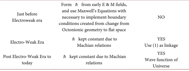
4) What the author would be particularly interested in knowing would be if actual semi classical reasoning could be used to get to an initial prequantum cosmological state. This would be akin to using [8], but even more to the point, using [9] and [10], with both these last references relevant to forming Planck’s constant from electromagnetic wave equations. The author points to the enor- mous Electromagnetic fields in the electroweak era as perhaps being part of the background necessary for such a semi classical derivation, plus a possible Octo-nionic space-time regime, as before inflation flattens space-time, as forming a boundary condition for such constructions to occur [11].
The relevant template for examining such questions is given in Table 1 as printed below.
5) The meaning of Octonionic geometry prior to the introduction of quantum physics presupposes a form of embedding geometry and in many ways is similar to Penrose’s cyclic conformal cosmology speculation Note the following argu-ment, as:
6) We are stuck with how a semi classical argument can be used to construct Table 1 below. In particular, we look at how Planck’s constant is derived, as in the electroweak regime of space-time, for a total derivative [9] [10]
(
)
(
)
y
y y
A
E A t x
t
ω
ω
∂
′
= = ⋅ ⋅ −
∂ (15)
Similarly [9] [10]
(
)
(
)
y
z y
A
B A t x
x
ω
ω
∂
′
= − = ⋅ ⋅ −
∂ (16)
The A field so given would be part of the Maxwell’s equations given by [9] as, when
[ ]
represents a D’Albertain operator, that in a vacuum, one would have for an A field [9] [10][ ]
A=0 (17)And for a scalar field φ
[image:6.595.209.537.614.738.2][ ]
φ=0 (18)Table 1. Time interval dynamical consequences do QM/WdW apply.
Just before Electroweak era
Form from early E & M fields, and use Maxwell’s Equations with necessary to implement boundary conditions created from change from
Octonionic geometry to flat space
NO
Electro-Weak Era kept constant due to Machian relations Use (1) as linkage YES
Post Electro-Weak Era to
today kept constant due to Machian relations
YES Wave function of
Following this line of thought we then would have an energy density given by, if ε0 is the early universe permeability [9]
(
2 2)
2 2(
(
)
)
0
0
2 Ey Bz Ay t x
ε
η= ⋅ + =ω ε⋅ ⋅ ′ ω⋅ − (19)
We integrate (19) over a specified E and M boundary, so that, then we can write the following condition namely [9] [10].
(
)
2(
(
)
)
(
)
d t x d dy z o Ay t x d t x d dy z
η
− =ωε
′ω
⋅ − −∫∫∫
∫∫∫
(20)(20) would be integrated over the boundary regime from the transition from the Octonionic regime of space time, to the non Octonionic regime, assuming an abrupt transition occurs, and we can write, the volume integral as representing [9] [10]
gravitational-energy
E = ⋅
ω
(21)Our contention for the rest of this paper, is that Mach’s principle will be ne-cessary as an information storage container so as to keep the following, i.e. hav-ing no variation in the Planck’s parameter after its formation from electrody-namics considerations as in (20) and (21). Then by applying [9] [10] we get
formed by semi classical reasons and need to have Machs principle (1) to have the same value up to the present era.
( )
t →Apply-Machs-Relations (Constant value) (22)
The question we can ask, is that can we have a prequantum regime com- mencing for (20) and (21) for if initial Planck
1 ~
# Ng
R <l ? And a closed 4 di-
mensional universe? If so, then what is the necessary geometrical regime of space-time so that the integration performed in (20) can commence properly? Also, what can we say about the formation of (21) above, as a number, # gets
larger and larger, effectively leading to 1 0 #
+
→ ? We need to know seriously how much space-time is needed to form (21) above? Do infinitesimal amounts of space-time suffice in order to fill in the following table as given below? If the answer is no, then when 1 0
#
+
→ leading to initial Planck #
1
~ 0
# Ng
R <l →∞→ ,
the semi classical derivation of (20) leading to (21) may not work. This is the ta- ble to consider if initial Planck #
1
~ small-value
# Ng
R <l ≠∞→ and not zero. Also,
with an Octonionic geometry regime which is a pre quantum state [11].
In so many words, the formation period for is our pre-quantum regime.
Table 1 could even hold if Rinitial→0 but that the 4 dimensional space-time
exhibiting such behavior is embedded in a higher dimensional template.
6. Having Not
R
initial→
0
, But
R
initial~
1
Ngl
Planck#
<
Growing Smaller, as
#
Becomes Larger
1) The initial entropy drops;
2) The number of bits initially available also drops.
Then, we argue that dramatically cutting the initial entropy and also the bits would lead to real trouble as far as preserving the formation of as given in [9] [10] and may lead to difficulties in application of (1) especially if bits for a computation for expansion cannot be formed in a general way at the start of in-flation. This uses the ideas in [11] and [12] precisely.
7. If
R
initial→
0
then If There Is an Isolated, Closed
Universe, There Is a Messy Situation
One does not have initial entropy, and the number of bits initially disappears. Abandoning the idea of a completely empty universe, this unperturbed point of matter-energy appears to be a recipe for a static point with no perturbation, as may be the end result of applying Fjortoft theorem [13] to the thermodynamic potential as given in [13], i.e. the non-definitive answer for fulfillment of criteria of instability by applying Fjortoft’s theorem [13] to the potential [11] leading to no instability as given by the potential given in [11] may lead to a point of space-time with no change, i.e. a singular point with “infinite” mass which does not change at all.
8. Can an Alternative to a Minimum Length Be Put in?
Consider the Example of Planck Time as the Minimal
Component, Not PLANCK Length
From J. Dickau, the following was given to the author, as a counter part as to how to view thresholds as to how a Mandelbrot set may pre select for critical behavior different from what is being pre supposed in this manuscript [14].
Dickau writes:
“If we examine the Mandelbrot Set along the Real axis, it informs us about behaviors that also pertain in the Quaternion and Octonic case-because the real axis is invariant over the number types. If numbers larger than 0.25 are squared and summed recursively (i.e. –z = z2 + c) the result will blow up, but numbers below this threshold never get to infinity, no matter how many times they are iterated. But once space-like dimensions are added i.e. an imaginary component- the equation blows up exponentially, faster than when iterated”.
Dickau concludes:
“Anyhow there may be a minimum (space-time length) involved but it is probably in the time direction”.
This is a counter pose to the idea of minimum length, i.e. the idea being a re-placement for what the author put in here: looking at a beginning situation with a crucial parameter Rinitial even if the initial time step is “put in by hand”. First of all, look at [4], if E is M, due to setting c = 1, then
(
)
2initial 4π initial initial
E
ρ
R R∆ ≈ ∆ (23)
choice as to Rinitial going to zero, or not going to zero will be conclusion of our article.
We have to look at what (23) tells us, even if we have an initial time step for which time is initially indeterminate, as given by a redoing of Mitra’s g00 formula [4] which we put in to establish the indeterminacy of the initial time step if quantum processes hold.
( ) ( )
(
)
00 0
2
exp 0
1 p
g
t p t ρ
ρ + =
−
= →
+
(24)
What Dickau is promoting is, that the Mandelbrot set, if applicable to early universe geometry, that what the author wrote, with
initial Planck #
1
~ small-value
# Ng
R <l ≠∞→ potentially going to zero, is less im-
portant than a minimum time length. To which the author states, if Dickau is correct as to applicability of the Mandelbrot set, that he, the author is happily corrected, but he also thinks that the Mandelbrot set is a beautiful example of the fungability of space-time metrics used. i.e. how one sets the initial space-time potential is to determine the correctness of the Mandelbrot set. i.e. the [13] ref-erence, as given, by Padmanabhan appears not to have a Mandelbrot set, in its thermodynamic potential. The instability issue is reviewed in Appendix II. For those who are interested in the author’s views as to lack proof of instability. It uses [13] which the author views as THE reference as far as thermodynamic po-tentials and the early universe.
9. We Need to Reconsider the Role of Quantum
Gravity Models at the Onset of Inflation
We are stuck in all Quantum gravity models as of putting in an initial time step
“by hand” so to speak which raises fundamental issues of what would form an initial time step in Quantum gravity. How the transition from the left to the right hand side of (22) occurs is crucial and it comes about because of a transi-tion from Octonionic geometry to quantum accessible and analyzable flat space geometry.
1) Having not Rinitial→0, but initial Planck
1 ~
# Ng
R <l grows smaller, as #
becomes larger leads to, if there is only an isolated 4 dimensional universe a situation for which:
The initial entropy drops;
And the number of bits initially available also drops.
We argue that dramatically cutting the initial entropy and also the bits would lead to real trouble as far as preserving the invariance of [15].
2) If Rinitial→0 then if there is an isolated, closed universe, one does not have initialentropy, and the number of bits initially disappears. i.e. in lieu of [11]
and [13] there may be no perturbation from an infinite point of space-time
10. Conclusions
1) The universe if Rinitial→0 [1] and if it is an isolated system, i.e. not as embedded in higher dimensions as referred to in [16] may have no bits, or computations as thought of by Ng [4]. This would be in tandem with the au-thor’s conclusion that one would have an initial infinite point mass and no evo-lution, and no generation of entropy.
2) If Rinitial→0 [1] but the universe is embedded in a higher dimensional system, as given by [16], then there is no reason to say there are no bits, or computations, and the universe will continue to evolve with entropy as a bypro-duct of that evolution.
3) The universe if one does not have Rinitial→0, i.e. if [1] does not hold, then there will be bits, entropy being generated, and also loop quantum gravity and quantum measures [17] so long as the minimum lP Planck length grid exists. The reacceleration of the universe commences as given in [18] due to DE being the same as vacuum energy. The author in Appendix III gives a derivation as to how the DE will be put in, via branes, which holds for both 8b and 8c , as a to be proven sideline.
4) Appendix IV lists the references that are pertinent to the study of
non-linear electrodynamics, which is useful for nonsingular starts to the begin-ning of the universe, and which is a mainstay of application the Author uses in other parallel publications. The reader is urged to review this partial list which is an important addendum in its own right.
Acknowledgements
This work is supported in part by National Nature Science Foundation of China Grant No. 11375279.
References
[1] Stoica, C. (2012) Beyond the FRWL Big Bang Singularity.
http://arxiv.org/pdf/1203.1819.pdf
[2] Beckwith, A.W. (2013) Is Quantum Mechanics Involved at the Start of
Cosmologi-cal Evolution? Does a Machian Relationship between Gravitons and Gravitinos Answer This Question? http://vixra.org/abs/1206.0023
[3] Lee, J.-W. (2012) On the Origin of Entropic Gravity and Inertia. Foundations of
Physics, 42, 1153-1164. http://arxiv.org/abs/1003.4464
https://doi.org/10.1007/s10701-012-9660-x
[4] Ng, Y.J. (2008) Spacetime Foam: From Entropy and Holography to Infinite Sta-
tistics and Nonlocality. Entropy, 10, 441-461. https://doi.org/10.3390/e10040441
[5] Mitra, A. (2011) Why the Big Bang Model Cannot Describe the Observed Universe
Having Pressure and Radiation. Journal of Modern Physics, 2, 1436-1442.
https://doi.org/10.4236/jmp.2011.212177
[6] Volovik, G.E. (2006) Vacuum Energy: Myths and Realities. arXIV: gr-qc/0604062 v2
[7] Beckwith, A. (2010) How to Use the Cosmological Schwinger Principle for Energy
Space-Time-Matter—Current Issues in Quantum Mechanics and Beyond, Castello Pasquini, 13-17 September 2010. http://iopscience.iop.org/1742-6596/306/1/012064
http://iopscience.iop.org/1742-6596/306/1;jsessionid=A05372A78C18D970BF35F40
A9A863B51.c
[8] Gryzinski, M. (1959) Classical Theory of Electronic and Ionic Inelastic Collisions.
Physical Review, 115, 374-383. https://doi.org/10.1103/PhysRev.115.374
[9] Bruchholz, U. (2009) Derivation of Planck’s Constant from Maxwell’s
Electrody-namics. Progress in Physics, 4, 67.
[10] Bruzchholz, U. (2009) Key Notes on a Geometric Theory of Fields. Progress in
Physics, 2, 107-113.
[11] Beckwith, A. (2011) Octonionic Gravity Formation, Its Connections to Micro
Phys-ics. Open Journal of Microphysics, 1, 13-18.
[12] Pringle, J. and King, A. (2007) Astrophysical Flows. Cambridge University Press,
New York. https://doi.org/10.1017/CBO9780511802201
[13] Padmanabhan, T. (2011) Lessons from Classical Gravity about the Quantum
Struc-ture of Space-Time. Journal of Physics: Conference Series, 306.
http://iopscience.iop.org/1742-6596/306/1/012001
[14] Dickau, J. (2012) Private Communication to the Author as to Minimum Space-
Time “Length” Provided as of August 7.
[15] Avessian, A.K. (2009) Planck’s Constant Evolution as a Cosmological Evolution
Test for the Early Universe. Gravitation and Cosmology, 15, 10-12.
https://doi.org/10.1134/S0202289309010034
[16] Durrer, R., et al. (2009) Dynamical Casimir Effect for Gravitons in Bouncing Brane Worlds. http://theory.physics.unige.ch/~durrer/papers/casimir.pdf
[17] Surya, S. (2010) In Search of a Covariant Quantum Measure. Journal of Physics:
Conference Series, 306, Article ID: 012018.
http://iopscience.iop.org/1742-6596/306/1/012018
[18] Beckwith, A.W. (2011) Identifying a Kaluza Klein Treatment of a Graviton
Permit-ting a Deceleration Parameter Q (Z) as an Alternative to Standard DE. The Journal
of Cosmology, 13, 1-15. http://journalofcosmology.com/BeckwithGraviton.pdf
[19] Corda, C. and Cuesta, H.J.M. (2011) Inflation from R2 Gravity: A New Approach
Using Nonlinear Electrodynamics. Astroparticle Physics, 34, 587-590.
https://doi.org/10.1016/j.astropartphys.2010.12.002
[20] Bessel Functions and Hankel Functions. http://dlmf.nist.gov/10.2
[21] Koury, J., Steinhardt, P.J. and Turkok, N. (2004) PRL92, 031302. hep-th/0307132.
[22] Koury, J., Steinhardt, P.J. and Turkok, N. (2003) PRL91, 161301. astro-ph/0302012.
[23] De Lorenci, V.A., Klippert, R., Novello, M. and Salim, J.M. (2002) Nonlinear
Elec-trodynamics and FRW Cosmology. Physical Review, 65, Article ID: 063501.
[24] Corda, C. and Cuesta, H.J.M. (2010) Removing Black-Hole Singularities with
Non-linear Electrodynamics,Modern Physics Letters A, 25, 2423.
https://arxiv.org/abs/0905.3298
Appendix I. Fjortoft Theorem
A necessary condition for instability is that if z∗ is a point in space-time for which 22
d 0 d
U
z = for any given potential U, then there must be some value z0
in the range z1<z0<z2 such that
( )
( )
0 2 0 2 d 0 d z UU z U z
z ⋅ − ∗ < (1)
For the proof, see [12] and also consider that the main discussion is to find instability in a physical system which will be described by a given potential U.
Next, we will construct in the boundary of the EW era, a way to come up with an optimal description for U
Appendix II. Constructing an Appropriate Potential for
Using Fjortoft Theorem in Cosmology for the Early
Universe Cannot Be Done. We Show Why
To do this, we will look at Padamanabhan [12] and his construction of (in Dice 2010) of thermodynamic potentials he used to have another construction of the Einstein GR equations. To start, Padamanabhan [5] wrote
If ab cd
P is a so called Lovelock entropy tensor, and Tab a stress energy tensor
( )
( )
( )
( )
( )
( )
( )
gravity matter gravity 4 ; 4a cd a b a b a b
ab c d ab ab
a a a b
matter ab
a a b a cd a b
ab ab c d
U P T x g
U U x g
U T U P
η
η
η
η η
λ
η η
η
η
λ
η η
η
η η
η
η
η
= − ⋅ ∇ ∇ + +
= + +
⇔ = = − ⋅ ∇ ∇
(1)
We now will look at
( )
( )
matter gravity ; 4a a b
ab
a cd a b
ab c d
U T
U P
η η η
η η η
=
= − ⋅ ∇ ∇ (2)
So happens that in terms of looking at the partial derivative of the top (1) eq-uation, we are looking at
( )
( )
2
2 aa aa
a
U
T λ x g
η
∂ = +
∂ (3)
Thus, we then will be looking at if there is a specified ηa
∗ for which the fol-lowing holds.
( )
( )
(
)
( )
0 2 0 0 20 0 0 0
4
0
a
cd a b a b
aa aa ab c d c d
a
a b a b a b a b
ab ab
U
T x g P
T x g
η
λ η η η η
η
η η η η λ η η η η
∗ ∗ ∗ ∗ ∗ ∗ ∂ = + ∗ − ⋅ ∇ ∇ − ∇ ∇ ∂
+ ⋅ − + ⋅ − <
(4)
What this is saying is that there is no unique point, using this ηa
∗ for which (4) holds. Therefore, we say there is no official point of instability of ηa
∗ due to (3). The Lagrangian structure of what can be built up by the potentials given in (3) with respect to ηa
re-spect to a 2nd derivative of a potential system. Such an inflection point designat-ing a speed up of acceleration due to DE exists a billion years ago [19]. Also note that the reason for the failure for (4) to be congruent to Fjoroft’s theorem is due to
( )
( )
2
2 0, for choices
a
aa aa
a
U
T λ x g η
η ∗
∂
= + ≠ ∀
∂
(5)
Appendix III. Modifying a Parallel Brane-Anti Brane
Argument to Obtain Massive Gravitons
Part I, of Appendix III. We come into this situation if, as in applying Fjorofts theorem, that we find Appendix II, Equation (5), holds, and then if so, we have to find another way to induce vacuum energy.
What (5), appendix II tells us is that there is an embedding structure for early universe geometry, some of which may take the form of the following diagram.
Part II of Appendix III. Working with a way to achieve energy injection into the universe, without appealing to Fjortoft theorem for alleged instabilities starting from Padmanabhan thermodynamic potential terms
Padmanabhan [13] introduced the following discussion as to entropy, namely starting with energy, we have
1 d
2 B loc
E= k
∫
nT (1)And the n value as in (7) is given by
d 32π ab cd d
cd ab
n= ⋅P ⋅ε ⋅ε ⋅ A (2)
where ab cd
P is a so called Lovelock entropy tensor, and εab a bi normal on the codimension −2 cross section, and then entropy is stated to be
2
d 32π ab cd dD
cd ab
S n P x
ν ν
ε ε σ −
∂ ∂
∝
∫
∝∫
⋅ ⋅ ⋅ (3)The end result, is that energy is induced via the temperature Tloc, while [13]
Local acceleration temperature 2π
loc
a n
T N
µ µ
= = (4)
Also, the change in n can be given by, if lP is the Planck’s length value [5] 2
P
n σd x l
∆ = (5)
Looking at (9) and (11) we state that the change in number count given in (4) is really a holographic surface phenomena, with N defined [13]
( )
1 2 BN=E k T (6)
The upshot is that we can, as implied by Ng [4] easily reference a change in entropy via [4]
~
S n (7)
temperature (4) is from another pre universe construction and that local insta-bility is ruled out by Appendix II, Equation (5). This leads us to ask as to what would be an acceptable way to form the formation of mass, i.e. say the mass of a graviton, via external factors introduced into our universe prior to the electro-weak era, in cosmology. To do that, look at if there are two branes on the AdS5 space-time so that with one moving and one stationary, we can look at Figure 1 as background as to introduce such external factors in our present space-time universe during its initial expansion phase
Part III, of Appendix III: Fall out from adopting Figure 1 and that due to no instability in the Padamanabhan supplied potentials. i.e. a way to obtain graviton mass via a root finding method.
Using [16] what we find is that there are two branes on the AdS5 space-time so that with one moving and one stationary, we can look at Figure 1 which is part of the geometry used in the spatial decomposition of the differential opera-tor acting upon the h• Fourier modes of the hij operator [16]. As given by [16], we have that
2 2 2 3
0
t k y y h
y •
∂ + − ∂ + ⋅∂ =
(8)
Using [16] the solution to (14) above takes the form of having
[
] (
)
2(
)
2
exp
ij ij
h•=H = ⋅e i⋅ ⋅ ⋅
ω
t m y⋅ ⋅ ⋅A J m y⋅ (9)ij
e is a polarization tensor, and the function J2
( )
my is a 2nd order Besselfunction [20]. A generalization offered by Durrer et al. [16] leads to
[
]
(
)
(
)
{
2}
(
)
22
π
exp 1
4
h= i⋅ ⋅ ⋅
ω
t m y⋅ ⋅ ⋅A J m y⋅ ⋅ + ⋅ m⋅ (10)
With the factor of π
(
)
21
4 m
+ ⋅ ⋅
coming in due to a boundary condition upon the wall of a brane put in, i.e. looking at [16]. With the right hand side of (10) due to a domain wall tension of a brane.
( )
5
2 yHij
κ π
ijT 0 [image:14.595.266.524.590.723.2]− ⋅∂ = ⋅ → (11) This will be in our example set as not equal to zero, in the right hand side, but equal to an extremely small parameter, namely
( )
5 ~
T yHij y yb κ πij ξ
+ =
∂ = ⋅ (12)
With this turned into
~
yhy yb
δ
+ =∂ (13)
The right hand side of (13) represents very small brane tension, which is un-derstandable. Then using [16] [20], i.e.
[ ]
( )
( )
{
2}
(
)
22
π
exp 1 ~
4
y y yb y
y yb
h = i tω my A J my m δ+
=
∂ = ∂ ⋅ ⋅ ⋅ ⋅ + ⋅ ⋅
(14)
And
( ) ( )
2( )
2( )
4( )
62 2 1 2 4 6
2 2! 2 3 2 2! 3 4 2 4! 3 4 5
my my my my
J my
= ⋅ − + − +
⋅ ⋅ ⋅ ⋅ ⋅ ⋅ ⋅ ⋅ ⋅ (15)
The upshot is, that afterwards,
( )
( )
( )
( )
( )
( )
( )
[
]
(
)
2 4 6
2 4 6
4
2 2 4 6
2 4 6
2
1
2 3 2 2! 3 4 2 4! 3 4 5
1
2 2! 2 4 6
2 3 2 2! 3 4 2 4! 3 4 5
exp π
1 4
δ+ ω
− + − + ⋅ ⋅ ⋅ ⋅ ⋅ ⋅ ⋅ ⋅ ⋅ ⋅ ⋅ ⋅ ⋅ − + − + ⋅ ⋅ ⋅ ⋅ ⋅ ⋅ ⋅ ⋅ ⋅ = ⋅ − ⋅ ⋅
my my my
my
y my my my
i t
m A
(16)
Should the term
[
]
(
)
20 exp π 1 0 4 i t m A δ
δ
ω
+ + → ⋅ ⋅ − ⋅ ⋅ → (17)
Then, (17) is acting much as in [16], whereas, one is recovering a simple nu-merical exercise as to obtain a suitable solution as given by (18), and (19) due to [3] where the domain tension of the brane vanishes. The novelty as to this ap-proach given in (17) is to obtain a time dependent behavior of the mass of the graviton,
( )
my f t( )
m f t( )
y= ⇔ ≡ (18)
Needless to say, (16) can only be solved for, numerically, i.e. fourth order po-lynomial solutions for quartic equations still give over simplified dynamics, es-pecially if (18) holds, and makes things more complicated. This is all being done to keep fidelity with respect to [16], as a possible feature of brane world dynam-ics as reflected in [16], as well as certain issues brought up in [8] as to what is a semi classical argument can obtain a usually quantum result. If this semi classic-al result is true, it has profound implications for [21], and [22] which are held to be M theory results with no classical analogues.
Appendix IV. Brief Listing of Non Linear Electrodynamics
References for Non Singular Start to the Universe
which complement the work done in this document
First of which is [19]. In it, important to the idea of R squared gravity having the consequence of a removal of early space-time singularities. The main result is in the quote that
“A non-singular early cosmology is proposed, where, adding a nonlinear elec-trodynamics Lagrangian to the high-order action, a bouncing is present and a power-law inflation is obtained. In the model the Ricci scalar R works like an in-flaton field.”
We will search for a similar identification in our future followups as to the importants of the Ricci scalar.
Secondly is [23] and [24]. [23] outlines the program of identifying electro-magnetic contributions to a non singular dense state of initial space-time mat-ter-energy, and [24] by Corda et al. specifically uses in its quote that:
“Such analysis will be improved by applying the Oppenheimer-Volkoff equa-tion to the black hole case. At the end, fixed the radius of the star, the final den-sity depends only on the introduced quintessential denden-sity term ργand on the mass.”
NLED identifies inputs for aquintessential density term ργ and we will be examining if our agument given in the text has any commonality with the Op-penheimer-Volkoff equation in a future update to our research endeavor.
Submit or recommend next manuscript to SCIRP and we will provide best service for you:
Accepting pre-submission inquiries through Email, Facebook, LinkedIn, Twitter, etc. A wide selection of journals (inclusive of 9 subjects, more than 200 journals)
Providing 24-hour high-quality service User-friendly online submission system Fair and swift peer-review system
Efficient typesetting and proofreading procedure
Display of the result of downloads and visits, as well as the number of cited articles Maximum dissemination of your research work
Submit your manuscript at: http://papersubmission.scirp.org/
![Figure 1. From [16].](https://thumb-us.123doks.com/thumbv2/123dok_us/7733994.706402/14.595.266.524.590.723/figure-from.webp)
