Existence and Stability of Equilibrium Points in the Robe’s
Restricted Three-Body Problem with Variable Masses
Jagadish Singh1, Oni Leke2
1Department of Mathematics, Faculty of Science, Ahmadu Bello University, Zaria, Nigeria
2Department of Mathematics, Statistics and Computer Science, College of Science, University of Agriculture, Makurdi, Nigeria Email: [email protected], [email protected]
Received January 4, 2013; revised February 6, 2013; accepted February 14, 2013
Copyright © 2013 Jagadish Singh, Oni Leke. This is an open access article distributed under the Creative Commons Attribution Li- cense, which permits unrestricted use, distribution, and reproduction in any medium, provided the original work is properly cited.
ABSTRACT
The positions and linear stability of the equilibrium points of the Robe’s circular restricted three-body problem, are gen- eralized to include the effect of mass variations of the primaries in accordance with the unified Meshcherskii law, when the motion of the primaries is determined by the Gylden-Meshcherskii problem. The autonomized dynamical system with constant coefficients here is possible, only when the shell is empty or when the densities of the medium and the infinitesimal body are equal. We found that the center of the shell is an equilibrium point. Further, when 1;
being the constant of a particular integral of the Gylden-Meshcherskii problem; a pair of equilibrium point, lying in the
-plane
with each forming triangles with the center of the shell and the second primary exist. Several of the points
exist depending on ; hence every point inside the shell is an equilibrium point. The linear stability of the equilibrium points is examined and it is seen that the point at the center of the shell of the autonomized system is conditionally sta- ble; while that of the non-autonomized system is unstable. The triangular equilibrium points on the
-plane
of both
systems are unstable.
Keywords: Robe’s Problem; Meshcherskii Law; GMP; Equilibruim Points
1. Introduction
The restricted three-body problem (R3BP) describes the motion of an infinitesimal mass moving under the gravi- tational effects of the two finite masses, called primaries, which move in circular orbits around their common cen- ter of mass on account of their mutual attraction and the infinitesimal mass not influencing the motion of the pri- maries. The R3BP is one of the most widely studied ar- eas in space dynamics as well as in celestial mechanics. The studies cover both analytical and numerical aspects. The analytic aspect considered mostly the circular, planar R3BP, in which all particles are confined to a plane and the primaries are in circular orbits around their centre of mass. The numerical aspect allowed consideration of the more general problem. The applications of the R3BP span solar system dynamics, lunar theory, motion of space craft and stellar dynamics.
Generally, we assume in the classical problem that the masses of celestial bodies don’t change with time. The phenomenon of isotropic radiation or absorption in stars led scientists to formulate the restricted problem of three
bodies with variable masses. During evolution, the masses of celestial bodies change, especially in a double star sys- tem were masses change rather intensively. Dufour [1] seems to have been the first to examine the astronomical phenomena of variable mass relating the secular variation of lunar acceleration with the increase of the Earth’s mass due to the impact of meteorites. Later, Gylden [2] estab- lished the differential equations of motion for the prob- lem when the mass are subject to variation. The inte- grable case to this differential equation was then given by Meshcherskii [3] for a particular mass variation law. Me- shcherskii [4] showed that the Gylden problem is a par- ticular case of the problem of two bodies with variable mass under the condition that the laws of variation are the same while the relative motion of the particles sepa- rating or attaching to them is zero everywhere. This law and its following generalization are referred to as Mesh- cherskii law. After this contribution, the physical mean- ing of the problem became clear and it is known as Gyl- den-Meshcherskii Problem (GMP).
allowed to vary. The interest in this model arises from cometary dynamics. When orbiting the Sun, comets lose part or even all of their mass due to thermal out-gassing of volatiles and due to interaction between the solar wind and the cometary surface. It also models an isotropic change in the mass of the gravitating bodies. That is, the primaries loss mass without causing a reactive force. Beside this, the GMP is used to describe the evolution of binary stars during secular mass loss owing to photon and corpuscular activity. This problem has also received considerable attention in the restricted three-body prob- lem. In this approach, the motion of the primaries is as- sumed to be determined by the GMP. Thus, one has to only study the motion of the body of infinitesimal mass which does not affect the motion of the primaries.
Gelf’gat [5] examined the restricted three-body prob- lem of variable masses in which the primary bodies move within the framework of the GMP and established the existence of five libration points (collinear & triangular) analogous to the classical libration points. Bekov [6] found two additional equilibrium points, called the co- planar points. A few recent characterizations of the GMP were examined by Gurfil and Belyanin [7] and Singh and Leke [8]. The majority of the authors have been inter- ested in the stellar applications of this problem than the solar system.
A new kind of the restricted three-body problem was formulated by Robe [9], in which one of the primaries of mass 1, is a rigid spherical shell, filled with homoge-
nous, incompressible fluid of density 1
m
, with the sec-
ond mass point 2 outside the shell and moving around
the first primary in a Keplerian orbit; and the infinitesi- mal mass 3 as a small solid sphere of an infinitesimal
radius, and of density 3 m
m
, moving inside the shell and is subject to the attraction of 2 and the buoyancy force
due to the fluid. He discussed the linear stability of an equilibrium point obtained in two cases; the first being
the case when the orbit of 2 around 1 is circular
and in the second case, when it is elliptic, but the shell is empty (there is no fluid inside it) or densities of 1 and
3 are equal. Since then, various studies under different
assumptions have been carried out by some researchers (e.g., Shrivastava and Garain [10]; Hallan and Rana [11]; Hallan and Mangang [12]). The Robe’s problem can be used to study the small oscillation of the Earth inner core taking into account the Moon’s attraction and the stabil- ity of the Earth’s centre (Robe [9]).
m
m m
m m
Modern concepts of the change in the distance be- tween the Earth and the Moon, and the change in their masses due to, out-gassing, impact of meteorites, aster- oids, comets and space dust lead to the necessity of in- vestigating dynamics problem in the Earth-Moon system under these conditions. It is believed that the Earth gains 100,000 kilograms of mass each year from space, one
million kilograms of mass every day due to in falling meteors. However, the Earth’s mass change appears to be exceedingly tiny, and seemingly, not nearly enough to change the dynamics in any significant way. Hence, in this paper, we investigate the motion of a test particle of infinitesimal mass under the set up of the Robe [9] model given that the masses of both primaries vary in propor- tion to each other according to the unified Meshcherskii [4] law and their motion determined by the Gylden-Me- shcherskii problem (Gylden [2]; Meshcherskii [3]). The existence and the long time stability behavior of equilib- rium points are investigated. This paper is a generaliza- tion of the paper by Robe [9], in the sense that the masses of the primaries are assumed to vary with time. Further, we restrict our study to the case when the shell is empty or when the densities of the medium and the infinitesimal body are equal. We found that every point inside the shell is an equilibrium point contrary to just one found at the center of the shell in the work of Robe [9].
The paper is organized as follows: Section 2 represents the equations of motion; the existence of the equilibrium points is mentioned in Section 3, while Section 4 inves- tigates their linear stability; Section 5 discusses the ob- tained results; and the conclusion is drawn in Section 6.
2. The Equations of Motion
The absolute motion of a body whose mass depends on time is described by the Meshcherskii equation for a point of variable mass, (see Sommerfeld [13]) as
m m
F v u v (1)
where is the velocity of the center of mass of the
absorbed mass immediately before its attachment with the body (or of the ejected mass immediately after its se- paration); is the velocity of the point measured in an inertial coordinate and
u
v
F is the combined force act-
ing on it which is also measured in an inertial coordinate system. There are two special cases of equation. How- ever, we shall consider in the case when mass is ejected with the same velocity of the body at any moment
uv
, that is, mass ejection does not produce a reac-tive force. This case can be used to study the motion of a body ejecting matters isotropically (or radiating energy).
Now, let m1
be the mass of the first primary which is
a rigid spherical shell of constant radius with center
at 1
M , and filled with a homogenous incompressible
fluid of constant density 1
and volume
f
V . Also, let
be the mass of the second primary with center at
2 2 m
M which describes a circular orbit around the first one.
the mass of the first primary is
1 s f
m t m t m (2)
where, m ts
is the mass of the shell; mf 1Vf
;
4π
3
f
V .
Now, if , then reactive forces are absent
from Equation (1) and the relative motion is described by the GMP (Gylden [2]; Meshcherskii [3]):
0
u v
1212 3
12 t r
r
r
(3)
where
t 1 2 ; 1 fm1
,
2 fm2
; f is
the gravitational constant and is the posi-
tion vector of relative to 12.
m
1 2
r M M
2 1
Further, we let 3 be the mass of the infinitesimal
body with center at 3
m m
M , having density 3 and sup-
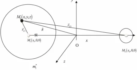
pose it is lying inside the spherical shell (see Figure 1).
Consequently, following Robe [9] and knowing that the distances between the centers of the primaries vary with time; then, the forces acting on the third body are
1) The force of attraction of m2 which is given by
2
2 3 2
3 23 m t m r
M M
F 3 (4)
2) The gravitational force FA exerted by the fluid of
density 1:
3
3 1 1 3 3 13 4π 3 A m f r
M M
F (5)
3) The buoyancy force exerted by the fluid, which is given by 3 2 3 1 1 3 13 3 4π . 3 B f m r
F M M (6)
[image:3.595.58.288.600.717.2]Now, the equation of motion of the third body in the inertial system taking into account the combined forces acting on it, is
Figure 1. The Robe R3BP.
3
2 32 1
13 3 3 3 32 13 4π 1 3 f r r r
R r (7)
where ROM3
In a synodic coordinates system 0xyz rotating with
angular velocity
t and origin at the center of mass,O, of the primaries; the equation of motion of m3 is
2 2 3 2 2 1 1 3 3 3 13 23 24π 1
3 t t t x x f x x r r r r
r r
(8)
where is the position vector of the third body rela- tive to the center of mass, r kˆ.
The Equation (8) in a Cartesian coordinate system, takes the form:
3 2 1 1 3 3 13 2 2 3 23 32 1 2
3 3 3 13 23 3 1 2 3 3 3 13 23 4π 2 1 3 4π 2 1 3 4π 1 3 f
x y x y x x
r x x r
y f y
y x y x
r r z f z z r r (9)
where the over-dot denotes differentiation with respect to time . The coordinates t
x y z, ,
of the third body isconnected with the distances between the center of the third body and centers of the primaries by the relation
22 2
13 1
r xx y z2, r232
xx2
2y2z 2while the barycentric x-coordinates x1 and x2 of the
primaries are connected with the distance between
them by the expressions 12
r
1 2 2 1
12 12
,
t t
x t x t
r t r t
(10)
Now, our aim is to transform Equation (9) to the au- tonomized form with constant coefficients using a Me- shcherskii’s transformation; the particular solutions of the GMP and the unified Meshcherskii [4] law. However, this is possible here, only when the densities of the me- dium and the infinitesimal body are equal, or the shell is empty
10
. Proceeding in this regards, using a Me- shcherskii’s transformation:
d 2
d
t x R t y R t z R t R t
(11)
13 13
r R t , r2323R
t ;
0 1 1
2 2
12 12
2 ,
t x R t x R t r R t R t
(12) and the unified Meshcherskii [4] law:
0
10
1 2
, ,
t t t
R t R t R t
20
(13)
where
20 10 20
2 : , , , , ,
R t t t are
constants,
The system of Equation (9), when the shell is empty in the autonomized forms:
0 0 2 , 2 . , (14) where
2
2 2 2
2 2 2 0 32 2 2 20
22 2
13 1 ,
2
2
2 213 2 ,
2 20 1 12 0
, 10
2 12
0
, 12 is constant and the
dashes denote differentiation with respect to .
Without loss of generality, we introduce the mass pa-
rameter , defined as 20
0
, 10
0
1
: 0 1, and make choice at initial time 0 respectively for the unit of mass, distance and time such that
t
0 f
,
12 1
, 0 1 Consequently,
2 20
1 , 2 1 , 1, 0 and
(15) The last Equation of (15) differs from the mass ratio given in Robe [9].
The equations of motion in the dimensionless Carte- sian coordinates are
2 , 2 ,
(16)
where
2 2
232 1 2 2
22 2
13 2,
2
223 1 ,
3. Equilibrium Points
The positions of the equilibrium points are the solutions of the equations
0
(17) That is,
32 2 2 2
3
2 2 2 2
3
2 2 2 2
1 0, 1 1 0 1 1 0 1 , . (18)
The last equation shows that if , it must have a
solution
1 0
, otherwise it has a different solution.
Therefore, the equilibrium points are the solutions of the following systems of equations:
2 2 2 231
0, 0, 0
1 (19)
32 2 2 2
3
2 2 2 2
1
0, 1
1 0, 0, 0, 1.
1 (20)
32 2 2 2
3
2 2 2 2
1 0, 1 1 0, 1 0, 0, (21)
Now, substituting the second Equation of (21) in its first one, we have
2 2 23 1 0 1 (22)which is not possible since 0
2 2
1
. Hence, we search
Figure 2. Equilibrium points on the -plane.
3.1. Point at the Center of the Shell
The equilibrium point at the center of the shell is found by solving Equation (19). To do this, we denote its first equation when 0 by f
, that is
2 01
f
(23)
Now, f
0 for 1 . Therefore, f
isincreasing in the open interval
,1
.As , f
and as
1
, . Consequently,
f f
is zero only once inthe interval
,1
. Hence, Equation (23) has only one root in this interval. Solving it, we get . (24) This gives the equilibrium point at the center of the spherical shell and is fully analogous to that obtained by Robe [9].
3.2. Triangular Points
The triangular points are found in the classical restricted three-body problem, but the existence of these points was not pointed out in the Robe [9] problem. However, the investigations concerning these points, when the shell is not empty, were carried out by Hallan and Rana [11]. The positions of the triangular equilibrium points in our case are the solutions of Equation (20). Here, we suppose that 1 0 and 0. Solving its second equation for 23, we at once have
1 3 23
1
(25)
Substituting Equation (25) in the first Equation of (20), results in
1 1
(26) Equation (26) gives the abscissae of the triangular points, which is less than the coordinate of the second
primary (i.e., 1 ) for 1 and lies within
the shell.
Now, knowing that 23
1
22 , substi-tuting Equations (25) and (26) in it and solving, we get
1 2 2 3 2 3
2 2
2 3 1
1
(27)
Equation (26) and (27) give the position of a pair of equilibrium points
,0,
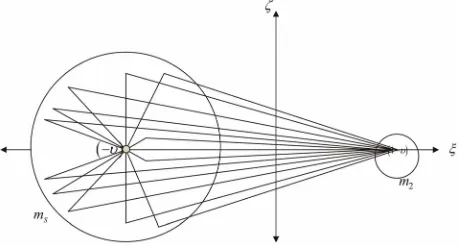
which exist for 1 and lies in the -plane, with each forming triangles with the center of the shell and the second primary; that is why we call them “triangular points” (see Figure 2: notdrawn to scale and Figures 3 and 4, drawn to scale). We
observe that the every point in the shell that is not col- linear with the center of the shell is a triangular equilib- rium points because they form triangles with the centers of both primaries, though this depends on the parameter
. Numerically, in the Earth-Moon system when
0.01
and 0 , the triangular points exist for
1.0035 1.01 . When 1.01 , we have
−0.0099 and 0.0827985 which lies inside the
shell. However, when 0.3, these points exist for
1.115 1.42 1
, (see Tables 1 and 2 in Section 4.2).
When , we have 0 which lies outside the
shell and since
L
, it is seen that infinite remote equilibrium points do not exist for any value of
0 1.
-0.002 0 0.002 0.004 0.006 0.008 0.01
x -1
-0.5 0 0.5
1
[image:5.595.323.530.586.716.2]z
Figure 3. Equilibrium points on the -plane for .
0.01
-0.3 -0.275 -0.25 -0.225 -0.2 -0.175 -0.15 -0.125 x
-1 -0.5 0 0.5 1
z
points and the characteristic roots
Table 1. Positions of triangular 1,2 1, 3,4 2, 5,6 3 for 0.01.
, p1 p2 p3 1 2 3
1 0 Infinity - - - - - -
1. −0.
0 −1. 92 0.989164 1.11562 0.953427
- -
001 00099 1.9138 - - - - - -
1.0035 −0.00347 1.0155 - - - - - -
1.0036 −0.00356 .996806 98 1.230.09i 0.792 0.09 i
1.01 −0.0099 0.0827985 −1.97 0.999591 1.63765 1.01912 1.24 0.08 i 0.814 0.07 i
1.011 Negative Imaginary - - - -
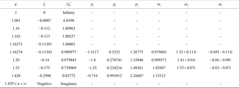
Table 2. Positions of triangular points and the characteristic roots 1,2 1, 3,4 2, 5,6 3 for 0.3.
p1 p2 p3 1 2 3
1 0 Infinity - - - - - -
1. −0. 7
−
−1. 17 0.3532 1.26775 0.979603 0
001 000 6.6598 - - - - - -
1.16 −0.112 1.00963 - - - - - -
1.162 −0.113 1.00257 - - - - - -
1.16273 0.11391 1.00001 - - - - - -
1.16274 −0.11392 0.999977 51 1.330.111i 0.691 0.111 i
1.20 −0.14 0.879845 −1.4 .278741 1.35846 0.999571 1.41 0.01 i 0.66 0.09 i
1.25 −0.175 0.738069 −1.25 0.234216 1.49261 1.02947 1.53 0.07 i 0.62 0.07 i
1.428 −0.2996 0.03772 −0.716 0.993912 2.26607 1.15512
1.429 Negative Imaginary - - - - - -
The equilibrium point at the center of the shell and the triangular equilibrium points of the system of Equation (9) when the densities of the medium and the infinitesi- mal body are equal, or the shell is empty
10
, aresought using the Meshcherskii’s [4] transf , in
the forms:
ormation
, 2
2
, 2,3
(2,3)
1x t R t x t R t z t R t
(28)
where, 2, and are the triangular points o
4. Stability of Equilibrium Points
nfinite
(29)
where the partial derivatives are evaluatedat the equi- librium point under consideration.
4.1. Equilibrium Point at the Center of
In order to consider the motion near the equilibrium point at the center of the shell, we let solutions of the first two
2,3
s. T
f the
autonom system he equilibrium points in this case
are function of time t.
ized
Let the third body be displaced to
0 u,0v,0w ents in the coordinates where u v w, , are small displacemof the i simal mass. Then, Equation (20) in the lin-
earized form are
0 0 0
0 0 0
0 0 0
2 ,
2 ,
.
u v u v w
v u u v w
w u v w
the Shell
equations of (29) be uAexp
, vBexp
,where ,A B and are constants. Taking first and se-
cond derivatives of the above, substituting them into the first two equations of system (29) and simplifying we ob-tain the matrix which has non-zero solution when
2 0 0
0
2
2
(3 )
Expanding the determinant, the characteristic equation corresponding to the variational equations when motion is considered in the -plane
2 0 0
0
is
24 0 0 4 2 0 0 0
Now, the values of the second order partial derivatives co
su
(31)
[image:6.595.58.539.256.434.2]
0 0
0
1 2 , 1 ,
1 1
, 0 0
0 0.
(32)
Substituting Equation of (32) in the variatio tio
, (33)
. w
nal Equa- n (29), at once results in
2 1 2 ,
u v u
2 1
v u v
1
1w (34)
Equation (34) is independent of Equation (33) and de- picts that the motion parallel to the axis is stable when
1
1
1
for 0 1, and unstable when
the converse holds.
Now, the characteristic Equation (3 tution of Equation (32) becomes
where
1) with the substi-
4 2 0
P Q
(35)
2
4 2 , 1 1 2
P Q ,
, Q0, while 0
Here P when
4
2
respectively.
The roots of Equation (35) are
2 1,2 2 4 2 D (36) w
(37)Now, when only when
here
1
, D is zero
16 1 9 8
D
8 9
. When 1 , the discriminant vanishes when
4
1 9 8
9
c
(38)
where c is the different values of
, at which thediscrim nant is zero.i c
ffe
are the criti
ters w xist for di rent values of Equation (38)
ca
.
l mass parame- hich e
exists only for 8
9
.
Now from Equation (37), we have
d 2 9 4
d and is zero when
D , (39)
4 9
. Therefore, Equation (39) is
positive when 4 and negative when
9 4 9 .
Th sing when the for-
mer holds and strictly decreasing w Now, when
is means that D is strictly increa
hen the later occurs. 0
in Equation (37)
(40) , we have
16 1
D
However, when 4
9
, Equation (37) reduces to
16 9 10
9
)
D (41
and is negative when 10
9
. Further, as increases
c
, D
to increases from the va
as
lue in (41) to 0. Finally,
c
increases to 1, the discriminant increases from
ze
6
ro to
2
9 24 1
D (42)
An inspection of Equation (42) reveals that for
0 , we have
Now, since the nature of the roots depend on the na- t, ma
0 D .
ture of the discriminan ss ratio, and the constant
of a particular inte ble w
gral of the Gylden-Meshcherskii
pro m; e consider the three regions of Equation (37)
coupled with the changes in P, which depends on
and .
1) When simultaneously 24 or
4 2
and 0 c,D0; h roots are respectively t e
1 2 1,2 1 1 2 3,4 1 12 4 ,
2 1 2 4 2 i i (43) and 1 2 1 3,4 1 2 2 1 2 i 1,2 1 2
1 4 ,
4 2 i
where i1 D.
The real parts of the two of the roots a
equal in both cases. Therefore, the equilibrium point is unstable.
hen
re positive and
2) W c, D0. The following cases are
e. a) If possibl 4 2
, two of the roots are ,
while the other two are negative and equal as well. The ium point is unstable in this case.
real and equal
equilibr
b) If 4
2
, here all the roots are zero, and the
equilibrium point is unstable
c) If 4
2
, all four roots are im
po and equa
In this case we have 3) When
aginary, with two
sitive l and the other two negative and equal.
positive stable resonance.
, D is positive. Therefore,
1
c
when 4 2
, the roots are:
1, 2
n
i n
(44) 1,2,3,4
where
121
1,2 2
In this case both values of are negativ
P D
e and all
th istinct and imag
point is r, for
n
e roots are d ary. Therefore, the equi-
librium stable. Howeve
in 4 2
, there
are two positive equal roots and two negative equal roots.
When 4
2
, the roots are real and distinct and the
equilibrium point is unstable due to a positive root, in both cases.Hence, we conclude that the equilibrium point of the autonomized system is stable for
, 0, 0
1
c
provided 4
2
and unstable for
0 c and c 1 provided
4 2
. This
is characterized by the arbitrary constant of the
Gylden-Meshcherskii problem and the mass ratio . The range of the stable motion is given by
4 4 9 8 8
1, provided
9 9
(45)
1
, Equation es
9
When (45) becom 8 1
9 and is
motion . Hence, as reasing
Equation (45) is approaching zero and the regi n of sta- bility is increasing.
fully analogous to that of Robe [9], when the shell is
empty and is circular is inc
o
4.
For the stability of the triangular equilibrium po have the following values of the partial derivatives:
2. Stability of Triangular Points
ints, we
0 1, 0 0 0
,
2
5 3 4 30
2 3
3 1 1
1
(46)
5 3 1 30
2 3
3 1 1
2
2 3Substituting the trial solutions
4 3 0
2 3
1 1
3 1 1
exp ,uA
exp ,
vB wCexp
then substituting haracter 6 4 1 2 p p
, in the ariational Equ- the partial derivatives istic equation in this case:
v ations (29), and
(46), we obtain the c
2 3 0 p 3 5
(47)
where, p1
5 3 5
4 3 2
2
2 3 2 3
4 5 3
4 3
3 1 3 1
1
3 1 1
3
2 7 6
5 3 p 2 3
2 5 3 2 8 3
2 2
3 4 3 2 3
3 1 1 18 1 1
1
p
4 10 3
4 3
4 3 4 3
18 1 1 18 1 1
+
4 13 3
2
1 3 1 3 1 21 2
1
1,2 1 3
2
3 3 32
p p p N N 2 2
1 1 1 2
3,4 2 3 1 3 2 3 1 3 2 3 1 3
1 2
1 3 1 3
2
2 3 1 3 1 3 1 3
3 32 2 3 2
3
2 22 3 62
p p ip p
N N N
i p N N
N (48) 2 2
1 1 1 2
5,6 2 3 1 3 2 3 1 3 2 3 1 3
1 2
1 3 1 3
2
2 3 1 3 1 3 1 3
3 32 2 3 2
3
2 22 3 62
p p ip p
N N N
i p N N
N where
31 1 2 3
3 2
2 3
2 1 1 1 2 3
2 9 27
4 3 2 9 27
N p p p p
p p p p p p
The stability of the triangular pointsis determined by the roots (48) of the characteristic equation. The six roots of characteristic equation and the positions of the train- gular points are presented in Tables 1 and 2 numerically
for 0.01 and 0.3 respectively with various
values of the parameter . When 0.01 ts ex
the train-
d th eristic roo ist only for
gular po 1.0035 ints an 1 e charact .01
, because here 0 and 1
the roots
lies in sh
ex lues o
side the ist for va
ell. In Tabl
f
e 2, these points and
in the interval
1.16273,1 28.4
when the mass parameter 0.3 iangula is po ss pa
. Our nume points exist, the c tive and p
eter. It
rical analy-
oef-3 is posi-
is clear from sis re
ficient ne
tiv th cases of th
veals that
1 p is
e in bo
when the tr e, p2
th
e triang ts. He
i uilibriu
In the case of solu 8)
corre-L on of stable so
we ha
e table that for a specific set of values of the parameters at least one of the roots is real and positive or at one has a positive real part. We conclude that a positive root and positive real part of the complex roots induce instability
at th ular poin nce the motion of the infini-
tesimal mass around the tr angular eq m points is
unstable.
the stability of the tions (2
sponding to the equilibrium point at the center of the
shell, on the basis of yapunov’s definiti -
lution (Krasnov et al. [14]), ve
lim lim
tx t tR t (49)
Equation (49) proves the instability of the equilibrium point at the center of the shell varying with time accord- ing to the Lyapunov’s theorem as they tend to infinity as time t is tending to infinity, which is however not pos-
sible in reality. However, when t is tending to infinity, is approaching a finite value (Singh and Leke [8]) and the Lyapunov Characteristic Numbers are positive for so
are unstable induce instability to the solutions. This also app
of the triangular solutions. Hence, the eq of
e
xistence of two or more triang ass ratio provided shell. Numerically, lutions with negative exponents, negative for solutions with positive exponents and zero for solutions with os- cillatory and constant solutions. We conclude that solu- tions with positive exponents which
lies in the case uilibrium points the non autonomous system of equations are unstable with respect to time.
5. Discussion and Conclusion
We have derived the equations of motion of the infini- t simal mass under the effects of the buoyancy force ex- erted by the fluid, the gravitational attraction of the fluid and the attraction of the second primary; when the masses of the primaries vary with respect to time in the absence of reactive forces. We have found that the equa- tions of motion can be transformed, when the motion of the primaries is determined by the GMP, to the autono- mized forms, only when the shell is empty.
One equilibrium point which lies on the center of the spherical shell and fully analogous to that of Robe [9]
exists. Further, the e ular
points is found which depends on the m 1
, and if the points lie within the
when 0.01 and 1.01, there are two triangular point positioned at 0.0099 and 0.0827985. However, for 0 , there is more than just a pair of these points. When 0.3, infinitely many triangular points exist depending on the value of the constant of the GMP in the interval
1.16273,1.428
. These equilibrium points are different from those of restricted three-bodyThe linear stability of the equilibrium points obtained has been studied and it is seen that the tria
problem with variable masses and those of Robe [9].
ngular points of
celes
at the of this
s problem in rth under the at
Moon.
2. [2]
the autonomized and time dependent systems are un- stable. The point on the center of the shell of the auto- nomized systems is stable under some certain conditions, while that dependent on time is unstable. The masses of tial bodies are changing with time; therefore it is
hoped th results paper will be useful in the
study of the dynamic the Ea -
traction of the
REFERENCES
[1] M. Dufour, “Ch.: Comptes Rendus Hebdomadaires de L’,” Accademie de Sciences, Amsterdam, 1886, pp. 840-84 H. Gylden, “Die Bahnbewegungen in Einem Systeme von zwei Körpern in dem Falle, dass die Massen Ver Nderun- Gen Unterworfen Sind,” Astronomische Nachrichten, Vol.
109, 1884, 1884, pp. 1-6.
[3] I. V. Meshcherskii, “Ueber die Integration der Bewegungs- gleichungen im Probleme zweier Körper von ver nderli- cher Masse,” Astronomische Nachrichten, Vol. 159, No.
15, 1902, pp. 229-242. doi:10.1002/asna.19021591502
[4] I. V. Meshcherskii, “Works on the Mechanics of Bodies of Variable Mass,” GITTL, Moscow, 1952, p. 205. [5] B. E. Gelf’gat, “Modern Problems of Celestial Mechanics
and Astrodynamics,” Nauka
[6] A. A. Bekov, e Restricted Prob- , Moscow, 1973, p. 7. “Liberation Points of th
lem of Three Bodies of Variable Mass,” Soviet Astronomy,
Vol. 32, 1988, pp. 106-107.
[7] P. Gurfil and S. Belyanin, “The Gauge-Generalized Gyl- den-Meshcherskii Problem,” Advances in Space Research,
Vol. 42, No. 8, 2008, pp. 1313-1317.
doi:10.1016/j.asr.2008.01.019
[8] J. Singh and O. Leke, “Stability of the Photogravitational Restricted Three-Body Problem with Variable Masses,”
Astrophysics and Space Science, Vol. 326, 2010, pp. 305-
314.
[9] H. A. G. Robe, “A New Kind of Three Body Problem,” Ce- lestial Mechanics and Dynamical Astronomy, Vol. 16, No.
3, 1977, pp. 343-351. doi:10.1007/BF01232659
[10] A. K. Shrivastava and D. N. Garain, “Effect of Perturba- tion on the Location of Libration Point in the Robe Re- stricted Problem of Three Bodies,” Celestial Mechanics and Dynamical Astronomy, Vol. 51, No. 1, 1991, pp. 67-
73. doi:10.1007/BF02426670
nd Dynamical As-
pp. 145-155.
[11] P. P. Hallan and N. Rana, “The Existence and Stability of Equilibrium Points in the Robe’s\Estricted Problem Three- Body Problem,” Celestial Mechanics a
tronomy, Vol. 79, No. 2, 2001,
doi:10.1023/A:1011173320720
2007, pp. 512-516. doi:10.1016/j.pss.2006.10.002
[13] A. Sommerfeld, “Mechanics,” Academic Press, New
G. I. Makarenko, “A Book York, of Problems in Ordinary Differential Equations,” MIR
Publications, Moscow, 1983, p. 255. 1952.