About Factorization of Quantum States with Few Qubits

(1)

http://www.scirp.org/journal/jamp

ISSN Online: 2327-4379 ISSN Print: 2327-4352

About Factorization of Quantum

States with Few Qubits

G. V. López1*, G. Montes1, M. Avila2, J. Rueda-Paz2

1_{Departamen to de Física, Universidad de Guadalajara, Guadalajara, Mexico}

2_{Centro Univeristario UAEM Valle de Chalco, Valle de Chalco, Estado de México, México}

Abstract

Through the study of the factorization conditions of a wave function made up of two, three and four qubits, we propose an analytical expression which can characterize entangled states in terms of the coefficients of the wave function and density matrix elements.

Keywords

Entangled State, Factorized State, Decoherence, Quantum Computing and Information, Chain of Spins System

1. Introduction

In quantum mechanics, multiple dimensional or multiple particles systems are characterized by the tensor product of the Hilbert subspaces [1], where each subspace is associated to each element. It is well known [2] that when there is no interaction among these elements, the wave function is just the tensor product of the wave functions of each element; that is, the tensor product of the wave func-tion associated to each element determines the non-interacting characteristic of the elements in a quantum system. If interaction occurs at some time among these elements, this tensor product disappears, and the wave function becomes entangled [3]. So, it is necessary to point out that if the wave function is not torized, the wave function is entangled. In this way, the characterization of fac-torization is somewhat equivalent to the characterization of entanglement. In this paper, we will follow this line of ideas to determine the characterization of an entangled state [4]-[12].

2. Factorized State

When a quantum systems is made up of several quantum subsystems, where the How to cite this paper: López, G.V.,

Montes, G., Avila, M. and Rueda-Paz, J. (2017) About Factorization of Quantum States with Few Qubits. Journal of Applied Mathematics and Physics, 5, 469-480. https://doi.org/10.4236/jamp.2017.52042

Received: December 12, 2016 Accepted: February 21, 2017 Published: February 24, 2017

http://creativecommons.org/licenses/by/4.0/

(2)

ith-subsystem is characterized by a Hamiltonian Hi and a Hilbert space εi,

corresponding a two-states and having a basis

{ }

_0,1

i

i ξ

ξ ₌ , the Hilbert space is written as the tensorial product of each subsystem, ε ε= n⊗ ⊗ ε1 (for n- subsystems), The state in each subsystems is defined as a qubit in quantum computation and information theory [13] and is given by

2 2

0 1 , 1,

i ai bi ai bi

ψ = + + = (1) where

{

0 , 1

}

is the basis of the two-states Hilbert subspace εi. A general

state Ψ _{in the Hilbert space} ε_{can be written as}

2

, with 1,

C_ξ C_ξ

ξ ξ

ξ

Ψ =

∑

= ₍₂₎

where C s_ξ′ are complex numbers, and ξ is an element of the basis of ε,

1 1 , 0,1 1, , .

n n k k n

ξ = ξ ξ = ξ ⊗ ⊗ ξ ξ = =  (3) A full factorized state in this space is

1 ,

n

ψ ψ

Ψ = ⊗ ⊗ (4) where ψk is given by (1).

For n=2, one has a general state Ψ ∈ε,

1 00 2 01 3 10 411 ,

C C C C

Ψ = + + + ₍₅₎

where we have chosen to use decimal notation for the coefficients. Let us assume that this state can be written as

2 1 ,

ψ ψ

Ψ = ⊗ ₍₆₎

with ψk ,k=1, 2 given by (1). Then, substituting (1) in (6) and equaling

coef-ficients with (5), it follows that

1 1 2, , , .2 1 2 3 1 2 4 1 2

C =a a C =a b C =b a C =b b (7)

From these expressions one obtains a single condition for factorization,

1 4 2 3.

C C =C C (8)

Thus, if this condition is not satisfied, the state (5) represents an entangled state. So, one can use the following known expression [14] as a characterization of an entangled state

( )2

1 4 2 3

2 .

C_Ψ = C C −C C (9) For n=3, a general state in the Hilbert space ε is

1 2 3 4

5 6 7 8

00 001 010 011

100 101 110 111 ,

C C C C

Ψ = + + +

+ + + + (10)

where, we have chosen again decimal notation for the coefficients. Assuming that this wave function can be written as Ψ =ψ3 ⊗ψ2 ⊗ψ1 with ψk

given by (1), and after some identifications (as before) and rearrangements, one gets

3 5 7 3

1

3

2 4 6 8 3

, 0

C C C a

C

b

C =C =C =C =b =/ (11a)

5 6

1 2 2

2

3 4 7 8 2

, 0

C C

C C a

b

(3)

3

1 2 4 1

1

5 6 7 8 1

, 0

C

C C C a

b

C =C =C =C = b =/ (11c)

. In addition, they bring about the following eight independent relations

1 4 2 3 0, 0, 0, 01 6 2 5 1 8 2 7 3 6 4 5

C C −C C = C C −C C = C C −C C = C C −C C = (12)

3 8 4 7 0, 0, 0, 0.5 8 6 7 1 7 3 5 2 8 4 6

C C −C C = C C −C C = C C −C C = C C −C C = (13)

If one of these expressions is not satisfied, the wave function (10) represents an entangled state. Therefore, one can propose the following expression to cha-racterize an entangled state

( )3

1 4 2 3 1 6 2 5 1 8 2 7 3 6 4 5

3 8 4 7 5 8 6 7 1 7 3 5 2 8 4 6

2 2 2 2

2 2 2 2 .

C C C C C C C C C C C C C C C C C

C C C C C C C C C C C C C C C C

Ψ = − + − + − + −

+ − + − + − + − (14)

For n=4, a general state in the Hilbert space ε is of the form

1 2 3 4

5 6 7 8

9 10 11 12

13 14 15 16

0000 0001 010 0011

0100 0101 0110 0111

100 1001 110 1011

1100 1101 1110 1111 .

C C C C

Ψ = + + +

+ + + +

(15)

Assuming this function can be expressed as Ψ =ψ4 ⊗ψ3 ⊗ψ2 ⊗ψ1 with ψ_k ,k=1, 2, 3, 4 given by (1), and after some identifications and

rear-rangements, one gets

3 5 7 9 13 15

1 11

2 4 6 8 10 12 14 16

C C C C C C

C C

C =C =C =C =C =C =C =C

5 6 9 10 13

1 2 14

3 4 7 8 11 12 15 16

C C C C C

C C C

C =C =C =C =C =C =C =C

3 9 10

1 2 4 11 12

5 6 7 8 13 14 15 16

C C C

C C C C C

C =C =C = C =C =C =C =C

3 5 6 7 8

1 2 4

9 10 11 12 13 14 15 16

,

C C C C C

C C C

C =C =C =C =C =C =C =C

expressing similar parallelism we mentioned before. Each row gives us 28 rela-tions, having a total of 112 possible relarela-tions, and from these relarela-tions, one can get the following 36 independent conditions

1 4 2 3 0 4 13 7 10 0 1 6 2 5 0 4 14 6 12 0

C C −C C = C C −C C = C C −C C = C C −C C = _(16a) 1 8 3 6 0 4 15 3 16 0 1 10 2 9 0 4 16 8 12 0 C C −C C = C C −C C = C C −C C = C C −C C = (16b)

1 11 3 9 0 5 8 6 7 0 1 12 2 11 0 5 14 6 13 0

C C −C C = C C −C C = C C −C C = C C −C C = (16c) 1 14 9 6 0 5 15 7 13 0 1 15 5 11 0 5 16 7 14 0 C C −C C = C C −C C = C C −C C = C C −C C = (16d)

2 8 4 6 0 6 11 5 12 0 2 12 4 10 0 6 15 16 8 0 C C −C C = C C −C C = C C −C C = C C −C C = (16e)

2 13 5 10 0 6 16 8 14 0 2 14 6 10 0 7 16 8 15 0 C C −C C = C C −C C = C C −C C = C C −C C = (16f)

(4)

Again, if one of these expression fail to happen, (15) will represents an entan-gled state. Thus, one can propose the following expression to characterize an entangled state made up of 4-qubits basis

( )4

1 4 2 3 4 13 7 10 1 6 2 5 4 14 6 12 1 8 3 6 4 15 3 16

1 10 2 9 4 16 8 12 1 11 3 9 5 8 6 7 1 12 2 11

5 14 6 13 1 14 9 6 5 15 7 13 1 15 5 11 5 16 7 14

2 2 2 2 2 2

2 2 2 2 2

C C C C C C C C C C C C C C C C C C C C C C C C C

C C C C C C C C C C C C C C C C C C C C

Ψ = − + − + − + − + − + −

+ − + − + − + − + −

2 8 4 6 6 11 5 11 2 12 4 10 6 15 16 8 2 13 5 10

6 16 8 14 2 14 6 10 7 16 8 15 2 16 10 8 7 12 8 11

3 8 4 7 9 12 10 11 3 15 7 11 9 14 10 11 3 13 11 5

9 1

2 2 2 2 2

2

C C C C C C C C C C C C C C C C C C C C

C C

+ − + − + − + − + −

+ 5−C C11 13 +2C C10 16−C C12 14 +2C C11 16−C C12 15 +2C C10 15−C C11 14 +2C C13 16−C C14 15.

(17)

As we can see from these examples, the number of conditions needed to cha-racterize a factorized state (or entangled state) grows exponentially with the number of qubits. So, characterization of an entangled state for n-qubits in gen-eral becomes a very hard work. Now, in terms of the density matrix elements, one could have the characterization of entangled states made up of 2, 3 and 4 qubits as

( )2

₍

₎

11 44 22 33 12 43

2 2 Re .

C_ρ = ρ ρ +ρ ρ − ρ ρ (18)

( )

₍

₎

₍

₎

₍

₎

(

)

(

)

(

)

(

)

3

11 44 22 33 12 43 11 66 22 55 12 65 11 88 22 77 12 87

33 66 44 55 34 65 33 88 44 77 34 87 55 88 66 77 56 87

11 77 33 55 13 75 22 88 44 66

2 2 Re 2 2 Re 2 2 Re

2 2 Re 2 2 Re

C_ρ ρ ρ ρ ρ ρ ρ ρ ρ ρ ρ ρ ρ ρ ρ ρ ρ ρ ρ

ρ ρ ρ ρ ρ ρ ρ ρ ρ ρ ρ ρ ρ ρ ρ ρ ρ ρ ρ ρ ρ ρ ρ ρ ρ ρ ρ ρ ρ

= + − + + − + + −

+ + − + + − + + −

+ + − + + −

(

₂₄ρ₈₆

)

.

(19)

( )

₍

₎

₍

₎

₍

₎

(

)

(

)

(

)

4

11 44 22 33 12 43 44 13,13 77 10,10 47 13,10 11 66 22 55 12 65

44 14,14 66 12,12 46 14,12 11 88 33 66 13 86 44 15,15 33 16,16 43 15,16

11 10,10 22 99

2 2 Re 2 2 Re 2 2 Re

2

C_ρ ρ ρ ρ ρ ρ ρ ρ ρ ρ ρ ρ ρ ρ ρ ρ ρ ρ ρ

ρ ρ ρ ρ ρ ρ ρ ρ ρ ρ ρ ρ ρ ρ ρ ρ ρ ρ ρ ρ ρ ρ

= + − + + − + + −

+ + − + + − + + −

+ + −

(

)

(

)

(

)

(

)

(

)

(

)

(

)

12 10,9 44 16,16 88 12,12 48 16,12 11 11,11 33 99 13 11,9

55 88 66 77 56 87 11 12,12 22 11,11 12 12,11 55 14,14 66 13,13 56 14,13

11 14,14 99 66 19 14,6

2 Re 2 2 Re 2 2 Re

2 2 Re 2 2 Re 2 2 Re

2 2 Re 2

ρ ρ ρ ρ ρ ρ ρ ρ ρ ρ ρ ρ ρ ρ ρ ρ ρ ρ ρ ρ ρ ρ ρ ρ ρ ρ ρ ρ ρ ρ ρ ρ ρ ρ ρ ρ ρ ρ

+ + − + + −

+ + − + + − + + −

+ + − +

(

)

(

)

(

)

(

)

(

)

(

)

55 15,15 77 13,13 57 15,13 11 15,15 55 11,11 15 15,11

55 16,16 77 14,14 57 16,14 22 88 44 66 24 86 66 11,11 55 12,12 6,5 11,12

22 12,12 44 10,10 24 12,10 66

2 Re 2 2 Re

2 2 Re 2 2 Re 2 2 Re

2 2 Re 2

ρ ρ ρ ρ ρ ρ ρ ρ ρ ρ ρ ρ ρ ρ ρ ρ ρ ρ ρ ρ ρ ρ ρ ρ ρ ρ ρ ρ ρ ρ ρ ρ ρ ρ ρ ρ ρ

+ − + + −

+ + − + + − + + −

+ + − +

(

)

(

)

(

)

(

)

(

)

15,15 16,16 88 6,16 15,8

22 13,13 55 10,10 25 13,10 66 16,16 88 14,14 68 16,14

22 14,14 66 10,10 2,6 14,10 77 16,16 88 15,15 78 16,15

22 16,16 10,10 88 2,10 16

2 Re

2 2 Re 2 2 Re

2 2 Re

ρ ρ ρ ρ ρ ρ ρ ρ ρ ρ ρ ρ ρ ρ ρ ρ ρ ρ ρ ρ ρ ρ ρ ρ ρ ρ ρ ρ ρ ρ ρ ρ ρ ρ ρ

+ − + + − + + − + + − + + − + + −

(

)

(

)

(

)

(

)

(

)

(

)

,8 77 12,12 88 11,11 78 12,11

33 88 44 77 34 87 99 12,12 10,10 11,11 9,10 12,11 33 15,15 77 11,11 37 15,11

99 14,14 10,10 11,11 9,10 14,11 33 13,13 11,11 55 3

2 2 Re

2 2 Re 2 2 Re 2 2 Re

2 2 Re 2 2 Re

ρ ρ ρ ρ ρ ρ

ρ ρ ρ ρ ρ ρ ρ ρ ρ ρ ρ ρ ρ ρ ρ ρ ρ ρ ρ ρ ρ ρ ρ ρ ρ ρ ρ ρ ρ

+ + − + + − + + − + + − + + − + + −

(

)

(

)

(

)

(

)

(

)

,11 13,5

99 15,15 11,11 13,13 9,11 1513 10,10 16,16 12,12 14,14 10,12 1614

11,11 16,16 12,12 15,15 11,12 16,15

10,10 15,15 11,11 14,14 10,11 15,14 13,13 16,16 14,14 15,1

2 2 Re 2 2 Re

2 2 Re

2 2 Re 2

ρ ρ ρ ρ ρ ρ ρ ρ ρ ρ ρ ρ ρ ρ ρ ρ ρ ρ ρ

ρ ρ ρ ρ ρ ρ ρ ρ ρ ρ

+ + − + + −

+ + −

+ + − + + ₅−2 Re

(

ρ_13,14ρ_16,15

)

(5)

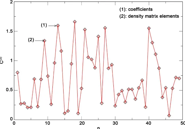
For other considerations of entanglement multiqubit entanglement see [6] [10] [15] [16]. Figure 1 below shows the values of the expressions (14) and (19) for 50 entangled states made up of 3-qubits basis and with values Cj, with

1, , 6

j=  randomly generated. As we can see, the values obtained with the

coefficients C sj′ and with the density matrix elements ρnm are the same.

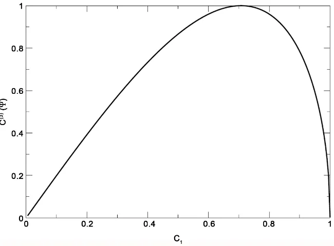
Figure 2 shows for the W state,

2 2

2

2 001 3 010 5100 , 1,2 3 5

W =C +C +C C +C +C = (21) the possible values of ( )3

( )

[image:5.595.212.535.233.458.2]

C Ψ . As we can see, there are four possible maxima corresponding to the values C2=C3=C5= ±1 3 and four maxima corres-

Figure 1. ( )3

[image:5.595.212.538.511.686.2]

C for arbitrary entangled state. Diamonds (density matrix) and circles (coefficients).

Figure 2. ( )3

C for the state W =C₁001 +C₂ 010 +C₃100 such that

2 2 2

1 2 3 1

(6)

ponding to the values C5=0, C2=C3= ±1 2, related to semi-factorized state 0 ⊗

(

C2 01 +C310

)

. Figure 3 shows the possible values of

( )3

_{( )}

C Ψ

for the state

2 2

1 000 8111 , 1 8 1.

GHZ =C +C C +C = (22) The maximum value of ( )3

( )

C Ψ is gotten for C1=C8 =1 2 , as one would expect.

For a Hilbert space

ε

generated by n-qubits, ( )n

C defines a continuous function C( )n :ε→ ℜ+ with ℜ =+

[

0,+∞

)

, c≥1. Since the coefficients of the wave function defines a compact set on the real space _ℜ2n_{due to the relation}

2

1 i iC =

∑

, the image of this compact set is a compact set in _ℜ+_[17]_{. Thus, a} normalization factor is possible to introduce on this function to define any compact set

[ ]

0,c , which it is not important.

3. Dynamical Consideration

Following Lloyd’s idea [18], consider a linear chain of nuclear spin one half, se-parated by some distance and inside a magnetic in a direction z ,

( )

(

k k k k

k k

H = −

∑

µ ⋅B z = −

∑

ω S .

[image:6.595.212.537.467.707.2]

If in addition, one has first and second neighbor Ising interaction, the Hamilto-nian of the system is just [19] [20].

Figure 3. ( )3

(7)

1 2

1 1 1

2 2

,

N N N

z z z z z

s k k k k k k

k k k

J J

H ω S S S S S

− −

+ +

2

1 2

1 1 1

1 1 1 .

2 2 2

k k k k k

N N N

k

k k k

J J

E_ξ ξ ω ξ ξ+ ξ ξ+

− ₊ − ₊

= = =

′

= −

∑

− − 

∑

− − 

∑

− ₍₂₄₎

Consider now that the environment is characterized by a Hamiltonian He

and its interacting with the quantum system with Hamiltonian Hs. Thus, the

total Hamiltonian would be H=Hs+He+Hse, where Hse is the part of the

Hamiltonian which takes into account the interaction system-environment, and the equation one would need to solve, in terms of the density matrix, is [21] [22]

[

,

]

,

t

i H

t

ρ _ρ

∂ ₌ ∂

 (25)

where ρt =ρt

( )

s e, is the density matrix which depends on the system and

en-vironment coordinates. The evolution of the system is unitary, but it is not possible to solve this equation due to a lot of degree of freedom. Therefore, un-der some approximations and tracing over the environment coordinates [23], it is possible to arrive to a Lindblad type of equation [24] [25] for the reduced den-sity matrix ρ

( )

s =tre

( )

ρt ,

[

]

† † †

1

1 1

,

2 2

I

s i i i i i i

i

i H V V V V V V

t

ρ _ρ _ρ _ρ _ρ

=

∂ ₌ ₊  ₋ ₋ 

 

∂

∑

 

 (26)

where Vi are called Kraus’ operators. This equation is not unitary and

Marko-vian (without memory of the dynamical process). This equation can be written in the interaction picture, through the transformation †

U U

ρ= ρ with

s

iH t

U=e , as

( )

,

i t

ρ _ρ

∂ = ∂

 _{ }

  (27)

where  

( )

ρ is the Lindblad operator

( )

† † †

1

1 1

2 2

I

i i i i i i

i

V V V V V V

ρ ρ ρ ρ

=

 

=  − − 

 

∑

 _  _  _ _ 

 (28)

with †

V=UVU . The explicit form of Lindblad operator is determined by the

type of environment to consider [26] at zero temperature. So, the operators can be Vi Si

−

= (for dissipation) for the model independent with the environment. In this case, each qubit of the chain acts independently with the environment, and one has local decoherence of the system. The Lindblad operator is

( )

1

(

)

2 2

N

k k k k k k k k

S S S S S S

i

ρ ₌

∑

γ −ρ +₋ + −ρ ρ₋ + −

 _  _ _{ } 



 ₍₂₉₎

where Sk

+  _and

k

(8)

ˆ

† i _kt

k k k

S±=US U± =S e± ± Ω

where ˆ

k

Ω is defined as ˆ

(

1 1

)

(

2 2

)

.

z z z z

k k k k k k

J J

w S ₊ S ₋ ′ S ₊ S ₋

Ω = + + + +

  . The

solu-tions of the equasolu-tions are

( )

(

)

( )

(

)

( )

(

)

( )

(

)

( )

(

)

( )

₍

_{( )}

₎

( )

( ) 1 2 3 1 2

1 3 2 3

1 2 3

11 11 22 33 44 55 66 77 88

55 66 77 88

33 44 77 88

22 44 66 88

77 88

66 88 44 88

88

0 0 0 0 0 0 0 0

0 0 0 0

0 0

0 0 0 0

0 ; t t t t t t t t e e e e e e e γ γ γ γ γ

γ γ γ γ

γ γ γ

ρ ρ ρ ρ ρ ρ ρ ρ ρ

ρ ρ ρ ρ

ρ ρ

ρ ρ ρ ρ

ρ − − − − + − + − + − + + = + + + + + + + − + + + − + + + − + + + + + + + + + −

( )

(

)

( ) ( )

(

)

( ) 14 2 3 1 1

1 58 2

14 14

2 2

1

0

0 1 ;

i

t i j j t

e

t e e

j j

φ _{γ γ}

γ γ ρ ρ ρ γ − ₋ ₊ ′ + −     = + −  ₊ ₊ _′   

( )

16

(

( )

)

( )

1 3

2

1 2

2 38 2

16 16 ₂ ₂

2

0

0 1 ;

4

i

t ij t

e

t e e

j φ γ γ γ γ ρ ρ ρ γ − ₋ ₊ −     = + −  +   

( )

(

)

( )

(

)

( ) 17 1 2 3 1

3 28 ₂

17 17 ₂

2 3

0

0 1 ;

i

t i j j t

e

t e e

j j

φ _{γ γ}

γ γ ρ ρ ρ γ − ₋ ₊ ′ + −         = + −  ₊ ₊ _′   

( )

(1 2 3)

1 2

18 18 0 ;

t

t e γ γ γ

ρ =ρ − + +

( )

(

( )

)

(

( )

)

( )

(

)

( )

_{( )}

( )

1 3

3

2 3 1 2 3

22 22 44 66 88 66 88

44 88 88

= 0 0 0 0 0 0

0 0 0 ;

t t

t e e

e e

γ γ γ

γ γ γ γ γ

ρ ρ ρ ρ ρ ρ ρ

ρ ρ ρ

− + − − + − + + + + + − + − + +

( )

(

)

( ) ( )

(

)

( ) 23 2 3 1 1

1 67 2

23 23 ₂

2 1

0

0 1 ;

i

t i j j t

e

t e e

j j

φ _{γ γ}

γ γ ρ ρ ρ γ − ₋ ₊ ′ − −     = + −  ₊ ₋ _′   

( )

(

)

(1 3) 2

1 2

25 25 0 47 0 1 ;

t t

t eγ e γ γ

ρ ₌_ρ ₊ρ ₋ − _ − +

 

( )

(1 2 3)

1 2

27 27 0 ;

t

t e γ γ γ

ρ =ρ − + +

( )

(1 2 3)

1 2 2

28 28 0 ;

t

t e γ γ γ

ρ =ρ − + +

( )

(

( )

)

(

( )

)

( )

(

)

( )

_{( )}

( )

1 2

2

2 3 1 2 3

33 33 44 77 88 77 88

44 88 88

0 0 0 0 0 0

0 0 0 ;

t t

t e e

e e

γ γ γ

γ γ γ γ γ

ρ ρ ρ

− + − − + − + + = + + + − + − + +

( )

(

)

( )

(

)

( ) 35 1 2 3 1

3 46 2

35 35 ₂

2 3

0

0 1 ;

i

t i j j t

e

t e e

j j

φ _{γ γ}

γ γ ρ ρ ρ γ − ₋ ₊ ′ −_ − + _     = + −  ₊ ₋ _′   

( )

(1 2 3)

1 2

36 36 0 ;

t

t e γ γ γ

(9)

( )

(1 2 3)

1 2 2

38 38 0 ;

t

t e γ γ γ

ρ =ρ − + +

( )

(

( )

)

(2 3)

(

( )

)

(

( )

)

( )

(

)

( )

_{( )}

( )

1 2

1

1 3 1 2 3

55 55 66 77 88 77 88

66 88 88

0 0 0 0 0 0

0 0 0 ;

t t

t e e

e e

γ γ γ

γ γ γ γ γ

ρ ρ ρ

− + −

− + − + +

= + + + − +

− + +

( )

( 1 2 3)

1 2 2

58 58 0 ;

t

t e γ γ γ

ρ =ρ − + +

( )

(

( )

)

(1 3)

_{( )}

(1 2 3)

66 66 0 88 0 88 0 ;

t t

ρ ₌ ρ ₊ρ − + ₋ρ − + +

( )

( 1 2 3)

1 2 2

67 67 0 ;

t

t e γ γ γ

ρ =ρ − + +

( )

( 1 2 3)

1

2 2

2

68 68 0 ;

t

t e γ γ γ

ρ =ρ − + +

( )

(

( )

)

(1 2)

_{( )}

(1 2 3)

77 77 0 88 0 88 0 ;

t t

ρ ₌ ρ ₊ρ − + ₋ρ − + +

( )

( 1 2 3)

1 2 2 2

78 78 0 ;

t

t e γ γ γ

ρ =ρ − + +

( )

(1 2 3)

88 88 0 .

t

t e γ γ γ

ρ ₌ρ − + +

where φij are given by

1 1 1

14 16 17

1 2 3

1 1

23 35

1 3

2

tan ; tan ; tan ;

tan ; tan .

j j j j j

j j j j

φ φ φ

γ γ γ

φ φ γ γ − − − − −    + ′   + ′ = _ _ = _ _ = _ _          − ′ − ′ = _ _ = _ _    

In our case, we have three qubits space

{

3 2 1

}

_0,1

i

ξ

ξ ξ ξ ₌ , and our parameter in units 2π MHz are

1 400; 2 200; 3 100 J 10; J 0.4

ω = ω = ω = = ′=

1 0.05; 0.05; 0.05.2 3

γ = γ = γ =

the time is normalized by the same factor of 2π MHz, and we include in this study the entangle state

(

)

1

000 111 001 110 . 2

[image:9.595.204.532.63.629.2]

Ψ = + + + ₍₃₀₎

Figure 4 shows the behavior of the entangled states W and GHZ as a

function of time when this entangled state interact with the environment. Purity behavior,

( )

2

(10)

[image:10.595.232.516.70.277.2]

Figure 4. ( )3

Cρ and Purity for the entangled state W , GHZ , and Ψ1 .

evolves in a mixed state and finishes in the pure ground state

(

000

)

, after sharing energy with the environment. The states GHZ and Ψ1 behave more robust than the state W , ( )3

Cρ grows since other entangled stated con- tribute to this function. In contrast, starting with the entangled state W , there

are not other entangled states which make contribution to the function ( )3

Cρ in the dynamics, and one sees an exponential decay.

4. Conclusion

We have studied the full factorization of a state made up of up to 4-qubits basic states. We have seen that there is an indication that the number of conditions to characterize a factorized state grows exponentially with the number of qubits. For two, three and four basic qubits, we showed the conditions in order to have a factorized state, and if any of one of these conditions fails, one gets instead an entangled state. Therefore, an entangled state is also characterized by the com-plement of each of this conditions, and the resulting expression has been de-noted by C( )n

(

n=2, 3, 4

)

. This non-negative function expressed in terms of the coefficients of the wave function or in terms of the density matrix elements represents a measurement of the entanglement of any wave function made up of basic n-qubits

(

n=2, 3, 4

)

. Using this function, we study the decay of entangled

states W , GHZ , and Ψ1 due to interaction with environment, and we noticed a great different behavior of the function ( )3

Cρ , indicating some type of robustness behavior of the states GHZ and Ψ1 . The main reason for this different behavior is that the entangled states GHZ and Ψ1 contain the ground state 000 , which is the final state in the dynamics.

References

(11)

[2] Messiah, A. (1958) Quantum Mechanics Vol. II. John-Wiley and Sons, New York. [3] Schrödinger, E. (1935)Die gegenwärtige Situation in der Quantenmechanik.

Na-turwissenschaften, 23, 807-812. https://doi.org/10.1007/BF01491891

[4] Horodecki, R., Horodecki, P., Horodecki, M. and Horodecki, K. (2009) Quantum Entanglement. Reviews of Modern Physics, 81, 865.

https://doi.org/10.1103/RevModPhys.81.865

[5] Wootters, W.K. (1998) Entanglement of Formation of an Arbitrary State of Two Qubits. Physical Review Letters, 80, 2245.

https://doi.org/10.1103/PhysRevLett.80.2245

[6] Seevinck, M. and Uffink, J. (2008) Partial Separability and Entanglement Criteria for Multiqubit Quantum States. Physical Review A, 78, Article ID: 032101.

https://doi.org/10.1103/physreva.78.032101

[7] Aolita, L., Chaves, R., Cavalcanti, D., Acín, A. and Davidovich, L. (2008) Scaling Laws for the Decay of Multiqubit Entanglement. Physical Review Letters, 100, Ar-ticle ID: 080501. https://doi.org/10.1103/PhysRevLett.100.080501

[8] Pope, D.T., Milburn, G.J. (2003) Multipartite Entanglement and Quantum State Exchange. Physical Review A, 67, Article ID: 052107.

https://doi.org/10.1103/PhysRevA.67.052107

[9] Love, P., van den Brink, A., Smirnov, A., Amin, A., Gra-jcar, M., Ilichev, E., Izmal-kov, A. and Zagoskin, A. (2007) A Characterization of Global Entanglement. Quantum Information Processing, 6, 187-195.

https://doi.org/10.1007/s11128-007-0052-7

[10] Ma, Z.-H., Chen, Z.-H. and Chen, J.-L. (2011) Measure of Genuine Multipartite Entanglement with Computable Lower Bounds. Physical Review A, 83, Article ID: 062325. https://doi.org/10.1103/physreva.83.062325

[11] Huber, M. and Mintert, F., Gabriel, A. and Hiesmayr, B.C. (2010) Detection of High-Dimensional Genuine Multipartite Entanglement of Mixed States. Physical Review Letters, 104, Article ID: 210501.

https://doi.org/10.1103/PhysRevLett.104.210501

[12] Chen, L. and Chen, Y.-X. (2007)Multiqubit Entanglement Witness. Physical Re-view A, 76, Article ID: 022330. https://doi.org/10.1103/PhysRevA.76.022330

[13] Nielsen, M. and Chuang, I. (2004) Quantum Computation and Quantum Informa-tion. Cambridge University Press, Cambridge.

[14] Alberio, S. and Fei, S.-M. (2001) A Note on Invariants and Entanglements. Journal of Optics B: Quantum and Semiclassical Optics, 3, 223-227.

[15] Horodecki, R., Horodecki, P., Horodecki, M. and Horodecki, K. (2009) Quantum Entanglement. Reviews of Modern Physics, 81, 865.

[16] Dür, W. and Chirac, J.I. (2000) Classification of Multiqubit Mixed States: Separabil-ity and DistillabilSeparabil-ity Properties. Physical Review A, 61, Article ID: 042314.

https://doi.org/10.1103/PhysRevA.61.042314

[17] Kolmogorov, A.N. and Fomin, S.V. (1970) Introductory Real Analysis. Dover Pub-lications Inc., Mineola.

[18] Lloyd, S. (1993) A Potential Realizable Quantum Computer. Science, 261, 1569.

https://doi.org/10.1126/science.261.5128.1569

[19] López, G.V. (2014) Diamond as a Solid State Quantum Computer with a Linear Chain of Nuclear Spins System. Journal of Modern Physics, 5, 55.

(12)

[20] Berman, G.P., Doolen, D.D., Kamenev, D.I., López, G.V. and Tsifrinovich, V.I. (2002) Perturbation Theory and Numerical Modeling of Quantum Logic Opera-tions with Large Number of Qubits. Contemporary Mathematics, 305, 13-41.

https://doi.org/10.1090/conm/305/05213

[21] Fano, U. (1957) Description of States in Quantum Mechanics by Density Matrix and Operator Techniques. Reviews of Modern Physics, 29, 74.

[22] Von Neumann, J. (1927) Wahrscheinlichkeitstheoretischer Aufbau der Quanten-mechanik. Göttinger Nachrichten, 1, 245.

[23] Davies, E.B. (1976) Quantum Theory of Open Systems. Academic Press, San Diego. [24] Heinz-Peter, B. and Petruccione, F. (2007) The Theory of Open Quantum Systems.

Oxford University Press, Oxford.

https://doi.org/10.1093/acprof:oso/9780199213900.001.0001

[25] Alicki, R. and Lendi, K. (2007) Quantum Dynamical Semigroups and Applications. In: Bartelmann, M., et al., Eds., Lecture Notes in Physics, Vol. 717, Springer, Berlin Heidelberg.

[26] Sumanta, D. and Agarwal, G.S. (2009) Decoherence Effects in Interacting Qubits under the Influence of Various Environments. Journal of Physics B: Atomic, Mole-cular and Optical Physics, 42, Article ID: 229801.

Submit or recommend next manuscript to SCIRP and we will provide best service for you:

Accepting pre-submission inquiries through Email, Facebook, LinkedIn, Twitter, etc. A wide selection of journals (inclusive of 9 subjects, more than 200 journals)

Providing 24-hour high-quality service User-friendly online submission system Fair and swift peer-review system

Efficient typesetting and proofreading procedure

Display of the result of downloads and visits, as well as the number of cited articles Maximum dissemination of your research work

Submit your manuscript at: http://papersubmission.scirp.org/