Math into L
A
TEX
This book is dedicated to those who worked so hard
and for so long to bring these important tools to us:
The L
ATEX3 team
and in particular
Frank Mittelbach (project leader) and David Carlisle
The
AMS
team
and in particular
George Gr¨atzer
Math into L
A
TEX
An Introduction to L
A
TEX and
AMS
-L
A
TEX
B I R K H ¨
A U S E R
George Gr¨atzer
Department of Mathematics University of Manitoba Winnipeg, Manitoba Canada R3T 2N2
Library of Congress Cataloging-in-Publication Data
Gr¨atzer, George A.
Math into LaTeX : an introduction to LaTeX and AMS-LaTeX / George Gr¨atzer
p. cm.
Includes index.
ISBN 0-8176-3805-9 (acid-free paper) (pbk. : alk. paper)
1. AMS-LaTeX. 2. Mathematics printing–Computer programs.
3. Computerized typesetting. I. Title.
Z253.4A65G69 1995 95-36881
688.202544536–dc20 CIP
Printed on acid-free paper c
°Birkh¨auser Boston 1996
All rights reserved.
Typeset by the Author in LATEX
Short contents
Preface xviii
Introduction xix
I
A short course
1
1 Typing your first article 3
II
Text and math
59
2 Typing text 61
3 Text environments 111
4 Typing math 140
5 Multiline math displays 180
III
Document structure
209
6 LATEX documents 211
7 Standard LATEX document classes 235
8 AMS-LATEX documents 243
vi Short contents
IV
Customizing
265
9 Customizing LATEX 267
V
Long bibliographies and indexes
309
10 BIBTEX 311
11 MakeIndex 332
A Math symbol tables 345
B Text symbol tables 356
C TheAMS-LATEX sample article 360
D Sample article with user-defined commands 372
E Background 379
F PostScript fonts 387
G Getting it 392
H Conversions 402
I Final word 410
Bibliography 413
Afterword 416
Contents
Preface xviii
Introduction xix
Typographical conventions . . . . xxvi
I
A short course
1
1 Typing your first article 3 1.1 Typing a very short “article” . . . . 41.1.1 The keyboard . . . . 4
1.1.2 Your first note. . . . 5
1.1.3 Lines too wide . . . . 7
1.1.4 More text features . . . . 9
1.2 Typing math. . . . 10
1.2.1 The keyboard . . . . 10
1.2.2 A note with math . . . . 10
1.2.3 Building blocks of a formula . . . . 14
1.2.4 Building a formula step-by-step . . . . 20
1.3 Formula gallery . . . . 22
1.4 Typing equations and aligned formulas . . . . 29
1.4.1 Equations . . . . 29
1.4.2 Aligned formulas . . . . 31
1.5 The anatomy of an article. . . . 33
1.5.1 The typeset article . . . . 38
1.6 Article templates . . . . 41
1.7 Your first article . . . . 42
1.7.1 Editing the top matter . . . . 42
viii Contents
1.7.2 Sectioning . . . . 43
1.7.3 Invoking proclamations. . . . 44
1.7.4 Inserting references . . . . 44
1.8 LATEX error messages . . . . 46
1.9 Logical and visual design . . . . 48
1.10 A brief overview . . . . 51
1.11 Using LATEX . . . . 52
1.11.1 AMS-LATEX revisited . . . . 52
1.11.2 Interactive LATEX . . . . 54
1.11.3 Files . . . . 54
1.11.4 Versions . . . . 55
1.12 What’s next? . . . . 56
II
Text and math
59
2 Typing text 61 2.1 The keyboard . . . . 622.1.1 The basic keys . . . . 62
2.1.2 Special keys . . . . 63
2.1.3 Prohibited keys . . . . 63
2.2 Words, sentences, and paragraphs . . . . 64
2.2.1 The spacing rules . . . . 64
2.2.2 The period . . . . 66
2.3 Instructing LATEX . . . . 67
2.3.1 Commands and environments . . . . 67
2.3.2 Scope . . . . 70
2.3.3 Types of commands. . . . 72
2.4 Symbols not on the keyboard. . . . 73
2.4.1 Quotes . . . . 73
2.4.2 Dashes. . . . 73
2.4.3 Ties or nonbreakable spaces . . . . 74
2.4.4 Special characters . . . . 74
2.4.5 Ligatures . . . . 75
2.4.6 Accents and symbols in text . . . . 75
2.4.7 Logos and numbers. . . . 76
2.4.8 Hyphenation . . . . 78
2.5 Commenting out . . . . 81
2.6 Changing font characteristics . . . . 83
2.6.1 The basic font characteristics . . . . 83
2.6.2 The document font families . . . . 84
2.6.3 Command pairs . . . . 85
Contents ix
2.6.5 Italic correction . . . . 86
2.6.6 Two-letter commands . . . . 87
2.6.7 Series . . . . 88
2.6.8 Size changes. . . . 88
2.6.9 Orthogonality . . . . 89
2.6.10 Boxed text. . . . 89
2.7 Lines, paragraphs, and pages . . . . 90
2.7.1 Lines. . . . 90
2.7.2 Paragraphs. . . . 93
2.7.3 Pages . . . . 94
2.7.4 Multicolumn printing. . . . 95
2.8 Spaces . . . . 96
2.8.1 Horizontal spaces . . . . 96
2.8.2 Vertical spaces. . . . 97
2.8.3 Relative spaces . . . . 99
2.8.4 Expanding spaces . . . . 99
2.9 Boxes . . . . 100
2.9.1 Line boxes. . . . 100
2.9.2 Paragraph boxes. . . . 103
2.9.3 Marginal comments. . . . 104
2.9.4 Solid boxes . . . . 105
2.9.5 Fine-tuning boxes. . . . 106
2.10 Footnotes . . . . 107
2.10.1 Fragile commands . . . . 107
2.11 Splitting up the file . . . . 108
2.11.1 Input and include . . . . 108
2.11.2 Combining files . . . . 109
3 Text environments 111 3.1 List environments . . . . 112
3.1.1 Numbered lists: enumerate . . . . 112
3.1.2 Bulleted lists: itemize . . . . 112
3.1.3 Captioned lists: description . . . . 113
3.1.4 Rule and combinations . . . . 114
3.2 Tabbing environment . . . . 116
3.3 Miscellaneous displayed text environments . . . . 118
3.4 Proclamations (theorem-like structures) . . . . 123
3.4.1 The full syntax . . . . 127
3.4.2 Proclamations with style . . . . 127
3.5 Proof environment . . . . 130
3.6 Some general rules for displayed text environments . . . . 131
x Contents
3.8 Style and size environments . . . . 138
4 Typing math 140 4.1 Math environments . . . . 141
4.2 The spacing rules . . . . 143
4.3 The equation environment . . . . 144
4.4 Basic constructs . . . . 146
4.4.1 Arithmetic . . . . 146
4.4.2 Subscripts and superscripts . . . . 147
4.4.3 Roots . . . . 148
4.4.4 Binomial coefficients . . . . 149
4.4.5 Integrals . . . . 149
4.4.6 Ellipses . . . . 150
4.5 Text in math. . . . 151
4.6 Delimiters . . . . 152
4.6.1 Delimiter tables . . . . 153
4.6.2 Delimiters of fixed size . . . . 153
4.6.3 Delimiters of variable size . . . . 154
4.6.4 Delimiters as binary relations . . . . 155
4.7 Operators . . . . 155
4.7.1 Operator tables . . . . 156
4.7.2 Declaring operators . . . . 157
4.7.3 Congruences . . . . 158
4.8 Sums and products . . . . 159
4.8.1 Large operators . . . . 159
4.8.2 Multiline subscripts and superscripts . . . . 160
4.9 Math accents . . . . 161
4.10 Horizontal lines that stretch . . . . 162
4.10.1 Horizontal braces . . . . 162
4.10.2 Over and underlines . . . . 163
4.10.3 Stretchable arrow math symbols . . . . 164
4.11 The spacing of symbols . . . . 164
4.12 Building new symbols. . . . 166
4.12.1 Stacking symbols . . . . 167
4.12.2 Declaring the type . . . . 168
4.13 Vertical spacing . . . . 169
4.14 Math alphabets and symbols . . . . 170
4.14.1 Math alphabets . . . . 171
4.14.2 Math alphabets of symbols . . . . 172
4.14.3 Bold math symbols . . . . 173
4.14.4 Size changes. . . . 175
Contents xi
4.15 Tagging and grouping . . . . 176
4.16 Generalized fractions . . . . 178
4.17 Boxed formulas . . . . 179
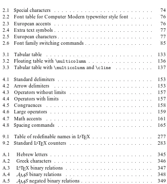
5 Multiline math displays 180 5.1 Gathering formulas . . . . 181
5.2 Splitting a long formula. . . . 182
5.3 Some general rules . . . . 184
5.3.1 The subformula rule . . . . 185
5.3.2 Group numbering . . . . 186
5.4 Aligned columns . . . . 187
5.4.1 The subformula rule revisited . . . . 188
5.4.2 Align variants . . . . 189
5.4.3 Intertext . . . . 192
5.5 Aligned subsidiary math environments. . . . 193
5.5.1 Subsidiary variants of aligned math environments . . . . . 193
5.5.2 Split . . . . 195
5.6 Adjusted columns . . . . 198
5.6.1 Matrices . . . . 198
5.6.2 Arrays . . . . 201
5.6.3 Cases . . . . 203
5.7 Commutative diagrams . . . . 204
5.8 Pagebreak . . . . 205
III
Document structure
209
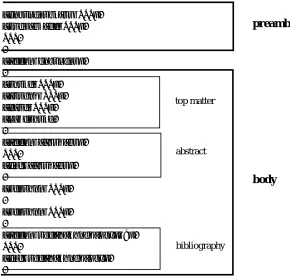
6 LATEX documents 211 6.1 The structure of a document . . . . 2126.2 The preamble . . . . 213
6.3 Front matter. . . . 214
6.3.1 Abstract . . . . 214
6.3.2 Table of contents . . . . 215
6.4 Main matter . . . . 217
6.4.1 Sectioning . . . . 217
6.4.2 Cross-referencing . . . . 220
6.4.3 Tables and figures. . . . 223
6.5 Back matter . . . . 227
6.5.1 Bibliography in an article . . . . 227
6.5.2 Index . . . . 231
[image:11.612.183.526.134.466.2]xii Contents
7 Standard LATEX document classes 235
7.1 Thearticle,report, andbookdocument classes . . . . 235
7.1.1 More on sectioning . . . . 236
7.1.2 Options . . . . 237
7.2 Theletterdocument class . . . . 239
7.3 The LATEX distribution . . . . 240
7.3.1 Tools . . . . 241
8 AMS-LATEX documents 243 8.1 The threeAMSdocument classes . . . . 243
8.1.1 Font size commands . . . . 244
8.2 The top matter . . . . 244
8.2.1 Article info . . . . 245
8.2.2 Author info . . . . 246
8.2.3 AMSinfo . . . . 249
8.2.4 Multiple authors . . . . 250
8.2.5 Examples . . . . 250
8.3 AMSarticle template . . . . 253
8.4 Options . . . . 257
8.4.1 Math options . . . . 260
8.5 TheAMS-LATEX packages . . . . 261
IV
Customizing
265
9 Customizing LATEX 267 9.1 User-defined commands . . . . 2689.1.1 Commands as shorthand . . . . 268
9.1.2 Arguments . . . . 271
9.1.3 Redefining commands . . . . 274
9.1.4 Optional arguments. . . . 275
9.1.5 Redefining names . . . . 276
9.1.6 Showing the meaning of commands . . . . 276
9.2 User-defined environments . . . . 279
9.2.1 Short arguments . . . . 282
9.3 Numbering and measuring . . . . 282
9.3.1 Counters . . . . 283
9.3.2 Length commands . . . . 287
9.4 Delimited commands . . . . 290
9.5 A custom command file. . . . 292
9.6 Custom lists . . . . 297
9.6.1 Length commands for thelistenvironment . . . . 297
Contents xiii
9.6.3 Two complete examples . . . . 301
9.6.4 Thetrivlistenvironment . . . . 304
9.7 Custom formats . . . . 304
V
Long bibliographies and indexes
309
10 BIBTEX 311 10.1 The database . . . . 31110.1.1 Entry types . . . . 312
10.1.2 Articles . . . . 315
10.1.3 Books . . . . 316
10.1.4 Conference proceedings and collections . . . . 317
10.1.5 Theses . . . . 319
10.1.6 Technical reports . . . . 320
10.1.7 Manuscripts . . . . 321
10.1.8 Other entry types . . . . 321
10.1.9 Abbreviations . . . . 322
10.2 Using BIBTEX. . . . 323
10.2.1 The sample files . . . . 323
10.2.2 The setup . . . . 325
10.2.3 The four steps of BIBTEXing . . . . 325
10.2.4 The files of BIBTEX . . . . 327
10.2.5 BIBTEX rules and messages. . . . 329
10.2.6 Concluding comments . . . . 331
11 MakeIndex 332 11.1 Preparing the document . . . . 332
11.2 Index entries . . . . 335
11.3 Processing the index entries . . . . 339
11.4 Rules. . . . 342
11.5 Glossary . . . . 344
A Math symbol tables 345
B Text symbol tables 356
C TheAMS-LATEX sample article 360
xiv Contents
E Background 379
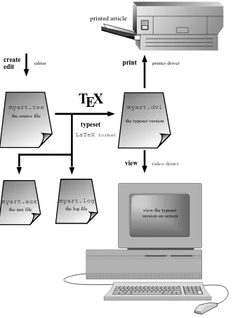
E.1 A short history . . . . 379
E.1.1 The first interim solution . . . . 381
E.1.2 The second interim solution . . . . 382
E.2 How does it work? . . . . 382
E.2.1 The layers . . . . 382
E.2.2 Typesetting . . . . 383
E.2.3 Viewing and printing . . . . 384
E.2.4 The files of LATEX . . . . 385
F PostScript fonts 387 F.1 The Times font and MathTıme. . . . 387
F.2 LucidaBright fonts . . . . 390
G Getting it 392 G.1 Getting TEX . . . . 392
G.2 Where to get it? . . . . 393
G.3 Getting ready . . . . 395
G.4 Transferring files . . . . 396
G.5 More advanced file transfer commands. . . . 398
G.6 The sample files . . . . 400
G.7 AMSand the user groups . . . . 400
H Conversions 402 H.1 From Plain TEX . . . . 402
H.1.1 TEX code in LATEX . . . . 403
H.2 From LATEX . . . . 403
H.2.1 Version 2e . . . . 404
H.2.2 Version 2.09 . . . . 404
H.2.3 The LATEX symbols . . . . 405
H.3 FromAMS-TEX. . . . 405
H.4 FromAMS-LATEX version 1.1 . . . . 406
I Final word 410 I.1 What was left out?. . . . 410
I.1.1 Omitted from LATEX . . . . 410
I.1.2 Omitted from TEX . . . . 411
I.2 Further reading . . . . 411
Bibliography 413
Afterword 416
List of tables
2.1 Special characters . . . . 74
2.2 Font table for Computer Modern typewriter style font . . . . 76
2.3 European accents . . . . 76
2.4 Extra text symbols. . . . 77
2.5 European characters. . . . 77
2.6 Font family switching commands. . . . 85
3.1 Tabular table . . . . 133
3.2 Floating table with\multicolumn . . . . 136
3.3 Tabular table with\multicolumnand\cline . . . . 137
4.1 Standard delimiters . . . . 153
4.2 Arrow delimiters . . . . 153
4.3 Operators without limits . . . . 157
4.4 Operators with limits . . . . 157
4.5 Congruences . . . . 158
4.6 Large operators . . . . 159
4.7 Math accents . . . . 161
4.8 Spacing commands . . . . 165
9.1 Table of redefinable names in LATEX . . . . 277
9.2 Standard LATEX counters . . . . 283
A.1 Hebrew letters . . . . 345
A.2 Greek characters . . . . 346
A.3 LATEX binary relations . . . . 347
A.4 AMSbinary relations . . . . 348
A.5 AMSnegated binary relations. . . . 349
[image:15.612.191.527.327.697.2]xvi List of tables
A.6 Binary operations . . . . 350
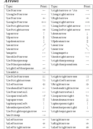
A.7 Arrows . . . . 351
A.8 Miscellaneous symbols. . . . 352
A.9 Math spacing commands . . . . 353
A.10 Delimiters . . . . 353
A.11 Operators . . . . 354
A.12 Math accents. . . . 355
A.13 Math font commands . . . . 355
B.1 Special text characters . . . . 356
B.2 Text accents . . . . 357
B.3 Some European characters . . . . 357
B.4 Extra text symbols. . . . 357
B.5 Text spacing commands . . . . 358
B.6 Text font commands . . . . 358
B.7 Font size changes . . . . 359
B.8 AMSfont size changes . . . . 359
F.1 Lower font table for the Times font . . . . 389
F.2 Upper font table for the Times font . . . . 389
G.1 Some UNIX commands . . . . 395
G.2 Someftpcommands . . . . 396
H.1 TEX commands to avoid in LATEX . . . . 404
H.2 A translation table. . . . 405
H.3 AMS-TEX style commands dropped inAMS-LATEX . . . . 407
List of figures
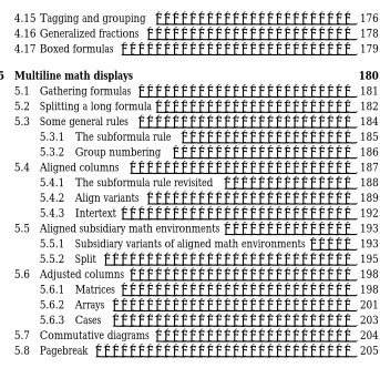
1.1 A schematic view of an article . . . . 34
1.2 The structure of LATEX . . . . 51
1.3 Using LATEX . . . . 53
6.1 The structure of a document . . . . 212
6.2 Sectioning commands in thearticledocument class . . . . 219
6.3 Sectioning commands in theamsartdocument class . . . . 219
6.4 Page layout for thearticledocument class . . . . 233
8.1 fleqnandreqnooptions for equations . . . . 258
8.2 Top-or-bottom tags option forsplit . . . . 258
8.3 AMS-LATEX package and document class interdependency . . . . 263
9.1 The layout of a custom list . . . . 298
10.1 Using BIBTEX, Step 2 . . . . 326
10.2 Using BIBTEX, Step 3 . . . . 326
11.1 A sample index . . . . 335
11.2 Using MakeIndex, Step 1 . . . . 340
11.3 Using MakeIndex, Step 2 . . . . 340
Preface
It is indeed a lucky author who is given the opportunity to completely rewrite a book barely a year after its publication. Writing about software affords such op-portunities (especially if the original edition sold out), since the author is shooting at a moving target.
LATEX andAMS-LATEX improved dramatically with the release of the new
stan-dard LATEX (called LATEX 2ε) in June of 1994 and the revision ofAMS-LATEX
(ver-sion 1.2) in February of 1995. The change inAMS-LATEX is profound. LATEX 2ε
made it possible forAMS-LATEX to join the LATEX world. One of the main points
of the present book is to make this clear. This book introduces LATEX as a tool
for mathematical typesetting, and treatsAMS-LATEX as a set of enhancements to
the standard LATEX, to be used in conjunction with hundreds of other LATEX 2ε
enhancements.
I am not a TEX expert. Learning the mysteries of the system has given me great respect for those who crafted it: Donald Knuth, Leslie Lamport, Michael Spivak, and others did the original work; David Carlisle, Michael J. Downes, David M. Jones, Frank Mittelbach, Rainer Sch¨opf, and many others built on the work of these pioneers to create the new LATEX andAMS-LATEX.
Many of these experts and a multitude of others helped me while I was writing this book. I would like to express my deepest appreciation and heartfelt thanks to all who gave their time so generously. Their story is told in the Afterword.
Of course, the responsibility is mine for all the mistakes remaining in the book. Please send corrections—and suggestions for improvements—to me at the follow-ing address:
Department of Mathematics University of Manitoba Winnipeg MB, R3T 2N2 Canada
e-mail: George [email protected]
Introduction
Is this book for you?
This book is for the mathematician, engineer, scientist, or technical typist who wants to write and typeset articles containing mathematical formulas but does not want to spend much time learning how to do it.
I assume you are set up to use LATEX, and you know how to use an editor to
type a document, such as:
\documentclass{article} \begin{document}
The square root of two: $\sqrt{2}$. I can type math! \end{document}
I also assume you know how to typeset a document, such as this example, with LATEX to get the printed version:
The square root of two: √2. I can type math!
and you can view and print the typeset document.
And what do I promise to deliver? I hope to provide you with a solid founda-tion in LATEX, theAMSenhancements, and some standard LATEX enhancements,
so typing a mathematical document will become second nature to you.
How to read this book?
Part I gives a short course in LATEX. Read it, work through the examples, and you
are ready to type your first paper. Later, at your leisure, read the other parts to become more proficient.
xx Introduction
The rest of this section introduces TEX, LATEX, and AMS-LATEX, and then
outlines what is in this book. If you already know that you want to use LATEX to
typeset math, you may choose to skip it.
TEX, L
A
TEX, and
AMS
-L
A
TEX
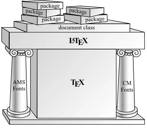
TEX is a typesetting language created by Donald E. Knuth; it has extensive capa-bilities to typeset math. LATEX is an extension of TEX designed by Leslie Lamport;
its major features include
a strong focus on document structure and the logical markup of text; automatic numbering and cross-referencing.
AMS-LATEX distills the decades-long experience of the American Mathematical
So-ciety (AMS) in publishing mathematical journals and books; it adds to LATEX a host
of features related to mathematical typesetting, especially the typesetting of multi-line formulas and the production of finely-tuned printed output.
Articles written in LATEX (andAMS-LATEX) are accepted for publication by
an increasing number of journals, including all the journals of theAMS.
Look at the typeset sample articles: sampart.tex(in Appendix C, on pages 361–363) andintrart.tex(on pages 39–40). You can begin creating such high-quality typeset articles after completing Part I.
What is document markup?
Most word processing programs are WYSIWYG (what you see is what you get); as you work, the text on the computer monitor is shown, more or less, as it’ll look when printed. Different fonts, font sizes, italics, and bold face are all shown.
A different approach is taken by a markup language. It works with a text edi-tor, an editing program that shows the text, the source file, on the computer moni-tor with only one font, in one size and shape. To indicate that you wish to change the font in the printed copy in some way, you must “mark up” the source file. For instance, to typeset the phrase “Small Caps” in small caps, you type
\textsc{Small Caps}
The\textsccommand is a markup command, and the printed output is
Small Caps
TEX is a markup language; LATEX is another markup language, an extension
Introduction xxi
\emph{complete-simple distributive lattices}
to emphasize the phrase “complete-simple distributive lattices”, which when typeset looks like
complete-simple distributive lattices
On pages 364–371 we show the source file and the typeset version of the
sampart.texsample article together. The markup in the source file may appear somewhat bewildering at first, especially if you have previously worked on a WYSI-WYG word processor. The typeset article is a rather pleasing-to-the-eye polished version of that same marked up material.1
TEX
TEX has excellent typesetting capabilities. It deals with mathematical formulas as well as text. To get√a2+b2 in a formula, type\sqrt{a^{2} + b^{2}}. There
is no need to worry about how to construct the square root symbol that covers a2+b2.
A tremendous appeal of the TEX language is that a source file is plain text, sometimes called an ASCII file.2 Therefore articles containing even the most
com-plicated mathematical expressions can be readily transmitted electronically—to col-leagues, coauthors, journals, editors, and publishers.
TEX is platform independent. You may type the source file on a Macintosh, and your coauthor may make improvements to the same file on an IBM compati-ble personal computer; the journal publishing the article may use a DEC minicom-puter. The form of TEX, a richer version, used to typeset documents is called Plain TEX. I’ll not try to distinguish between the two.
TEX, however, is a programming language, meant to be used by programmers.
L
ATEX
LATEX is much easier and safer to work with than TEX; it has a number of built-in
safety features and a large set of error messages.
LATEX, building on TEX, provides the following additional features:
An article is divided into logical units such as an abstract, sections, theorems, a bibliography, and so on. The logical units are typed separately. After all the
1Of course, markup languages have always dominated typographic work of high quality. On the
Internet, the most trendy communications on the World Wide Web are written in a markup language called HTML (HyperText Markup Language).
xxii Introduction
units have been typed, LATEX organizes the placement and formatting of these
elements.
Notice line 4 of the source file of thesampart.texsample article
\documentclass{amsart}
on page 364. Here the general design is specified by the amsart “document class”, which is theAMSarticle document class. When submitting your article to a journal that is equipped to handle LATEX articles (and the number of such
journals is increasing rapidly), only the name of the document class is replaced by the editor to make the article conform to the design of the journal.
LATEX relieves you of tedious bookkeeping chores. Consider a completed article,
with theorems and equations numbered and properly cross-referenced. Upon fi-nal reading, some changes must be made—for example, section 4 has to be placed after section 7, and a new theorem has to be inserted somewhere in the middle. Such a minor change used to be a major headache! But with LATEX, it becomes
almost a pleasure to make such changes. LATEX automatically redoes all the
num-bering and cross-references.
Typing the same bibliographic references in article after article is a tedious chore. With LATEX you may use BIBTEX, a program that helps you create and
main-tain bibliographic databases, so references need not be retyped for each article. BIBTEX will select and format the needed references from the databases.
All the features of LATEX are made available by theLaTeXformat, which you
should use to typeset the sample documents in this book.
AMS
-L
ATEX
TheAMSenhanced the capabilities of LATEX in three different areas. You decide
which of these are important to you.
1. Math enhancements. The first area of improvement is a wide variety of tools for typesetting math.AMS-LATEX provides
excellent tools to deal with multiline math formulas requiring special align-ment. For instance, in the following formula, the equals sign (=) is verti-cally aligned and so are the explanatory comments:
x= (x+y)(x+z) (by distributivity)
=x+yz (by Condition (M))
Introduction xxiii
numerous constructs for typesetting math, exemplified by the following formula:
f(x) =
−x2, ifx <0;
α+x, if 0≤x≤1;
x2, otherwise.
special spacing rules for dozens of formula types, for example
a≡b (mod Θ)
If the above formula is typed inline, it becomes:a≡b (mod Θ); the spac-ing is automatically changed.
multiline “subscripts” as in
X
i<n j<m
α2i,j
user-defined symbols for typesetting math, such as
Truncf(x), A,ˆˆ ∗X∗
formulas numbered in a variety of ways: – automatically,
– manually (by tagging),
– by groups, with a group number such as (2), and individual numbers such as (2a), (2b), and so on.
the proof environment and three theorem styles; see the sampart.tex
sample article (pages 361–363) for examples.
2. Document classes. AMS-LATEX provides a number of document classes,
in-cluding theAMSarticle document class,amsart, which allows the input of the title page information (author, address, e-mail, and so on) as separate entities. As a result, a journal can typeset even the title page of an article according to its own specifications without having to retype it.
Many users prefer the visual design of theamsartdocument class to the sim-pler design of the classical LATEXarticledocument class.
3. Fonts. There are hundreds of binary operations, binary relations, negated bi-nary relations, bold symbols, arrows, extensible arrows, and so on, provided byAMS-LATEX, which also makes available additional math alphabets such
as Blackboard bold, Euler Fraktur, Euler Script, and math bold italic. Here are just a few examples:
xxiv Introduction
We have barely scratched the surface of this truly powerful set of enhance-ments.
What is in the book?
Part I (Chapter 1) will help you get started quickly with LATEX; if you read it
carefully, you’ll certainly be ready to start typing your first article and tackle LATEX
in more depth.
Part I guides you through:
marking up text, which is quite easy;
marking up math, which is not so straightforward (four sections ease you into mathematical typesetting: the first discusses the basic building blocks; the sec-ond shows how to build up a complicated formula in simple steps; the third is a formula gallery; and the fourth deals with equations and multiline formulas); the anatomy of an article;
how to set up an article template; typing your first article.
Part IIintroduces the two most basic skills in depth: typing text and typing math.
Chapters 2 and 3 introduce text and displayed text. Chapter 2 is very im-portant; when typing your LATEX document, you spend most of your time typing
text. The topics covered include special characters and accents, hyphenation, fonts, and spacing. Chapter 3 covers displayed text including lists and tables, and for the mathematician, proclamations (theorem-like structures) and proofs.
Chapters 4 and 5discuss math and displayed math. Of course, typing math is the heart of any mathematical typesetting system. Chapter 4 discusses this topic in detail, including basic constructs, operators, delimiters, building new symbols, fonts, and grouping of equations. Chapter 5 presents one of the major contribu-tions ofAMS-LATEX: aligned multiline formulas. This chapter also contains other
multiline formulas.
Part IIIdiscusses the parts of a LATEX document. In Chapter 6, you learn
about the structure of a LATEX document. The most important topics are
section-ing and cross-referencsection-ing. In Chapter 7, the standard LATEX document classes are
presented: article,report,book, andletter, along with a description of the standard LATEX distribution. In Chapter 8, theAMSdocument classes are
dis-cussed. In particular, the title page information for the amsartdocument class and a description of the standardAMS-LATEX distribution is presented.
Part IV(Chapter 9) introduces techniques to customize LATEX to speed up
typing source files and typesetting of documents. LATEX really speeds up with
user-defined commands, user-user-defined environments, and custom formats. You’ll learn how parameters that effect the behavior of LATEX are stored in counters and length
Introduction xxv
In Part V (Chapters 10 and 11), we’ll discuss two programs: BIBTEX and
MakeIndex that complement the standard LATEX distribution; they give a helping
hand in making large bibliographies and indices.
Appendices A and Bwill probably be needed quite often in your work: they contain math symbol tables and text symbol tables.
Appendix C presents theAMS-LATEX sample article,sampart.tex, first in
typeset form (pages 361–363), then in “mixed” form, showing the source file and the typeset article together (pages 364–371). You can learn a lot about LATEX and
AMS-LATEX just by reading the source file a paragraph at a time and see how that
paragraph looks typeset. Then Appendix D rewrites this sample article utilizing the user-defined commands collected inlattice.styof section 9.5.
Appendix Erelates some historical background material on LATEX: how did
it develop and how does it work. Appendix F is a brief introduction to the use of PostScript fonts in a LATEX document. Appendix G shows how you can obtain
LATEX andAMS-LATEX, and how you can keep them up-to-date through the
In-ternet. A work session is reproduced (in part) using “anonymous ftp” (file transfer protocol).
Appendix Hwill help those who have worked with (Plain) TEX, LATEX
ver-sion 2.09,AMS-TEX, orAMS-LATEX version 1.1, programs from which the new
LATEX andAMS-LATEX developed. Some tips are given to smooth the transition
to the new LATEX andAMS-LATEX.
Finally, Appendix I points the way for further study. The most important book for extending and customizing LATEX is The LATEX Companion, the work of
xxvi Introduction
Typographical conventions
To make this book easy to read, I use some very simple conventions on the use of fonts.
Explanatory text is set in the Galliard font, as this text is.
This book is about typesetting math in LATEX. So often you are told to type
in some material and shown how it’ll look typeset.
I use this font, Computer Modern typewriter style, to show what you have to type. All characters have the same width so it’s easy to distinguish it from the other fonts used in this book.
I use the same font for commands (\parbox), environments (align), documents (sampart.tex), document classes (article), directories and folders (work), coun-ters (tocdepth), and so on.
The names of packages (amsmath), extensions of LATEX, are printed in a sans
serif font, as traditional.
When I show you how something looks when typeset, I use this font, Com-puter Modern roman, which you’ll most likely see when you use LATEX. This
looks sufficiently different from the other two fonts I use so that you should have little difficulty recognizing typeset LATEX material. If the typeset material is a
separate paragraph (or paragraphs), I make it visually stand out even more by adding the little corner symbols on the margin to offset it.
When I give explanations in the text: “Compareiffwithiff, typed asiffand
if{f}, respectively.” I use the same fonts but since they are not visually set off, it may be a little harder to see thatiffis in Computer Modern roman andiffis in Computer Modern typewriter style.
Commands are introduced, as a rule, with examples:
\\[0.5in]
However, sometimes it’s necessary to more formally define the syntax of a com-mand. For instance:
\\[length]
PART I
A short course
C H A P T E R
1
Typing
your first article
In this chapter, you’ll start writing your first article. All you have to do is to type the (electronic) source file; LATEX does the rest.
In the next few sections, I’ll introduce you to the most important commands for typesetting text and math by working through examples. Go to the latter parts of this book for more detail.
The source file is made up of text, math (for instance,√5), and instructions to LATEX. This is how you type the last sentence:
The source file is made up of \emph{text}, \emph{math} (for instance, $\sqrt{5}$), and \emph{instructions} to \LaTeX.
In this sentence,
The source file is made up of \emph{text}, \emph{math} (for instance,
is text,
$\sqrt{5}$
is math, and
4 Chapter 1 Typing your first article
\emph{text}
is an instruction (a command). Commands, as a rule, start with a backslash\and are meant to instruct LATEX; this particular command, \emph, emphasizes text
given as its argument (between the braces). Another kind of instruction is called an environment. For instance,
\begin{flushright}
and
\end{flushright}
bracket aflushrightenvironment—what is typed inside this environment comes out right justified (lined up against the right margin) in the printed form.
In practice, text, math, and instructions are intertwined. For example,
\emph{My first integral} $\int \zeta^{2}(x) \, dx$
which produces
My first integral R ζ2(x)dx
is a mixture of all three. Nevertheless, to some extent I try to introduce the three topics: typing text, typing math, and giving instructions to LATEX (commands and
environments) as if they were separate topics.
I introduce the basic features of LATEX by working with a number of sample
documents. If you wish to obtain these documents electronically, create a sub-directory (folder) on your computer, say, ftp, and proceed to download all the sample files as described in section G.6. Also create a subdirectory (folder) called
work. Whenever you want to use one of these documents, copy it from theftp
subdirectory (folder) to theworksubdirectory (folder), so that the original remains unchanged; alternatively, type in the examples as shown in the book. In this book, theftpdirectory and theworkdirectory will refer to the directories (folders) you hereby create without further elaboration.
1.1
Typing a very short “article”
First we discuss how to use the keyboard in LATEX, and then type a very short
“ar-ticle” containing only text.
1.1.1
The keyboard
1.1 Typing a very short “article” 5
a-z A-Z 0-9
+ = * / ( ) [ ]
You may also use the punctuation marks
, ; . ? ! : ‘ ’
-and the spacebar, the tab key, -and the return (or enter) key. There are thirteen special keys (on most keyboards):
# $ % & ~ ^ \ { } @ " |
used mostly in LATEX instructions. There are special commands to type most of
these special characters (as well as composite characters, such as accented charac-ters) if you need them in text. For instance,$is typed as\$, is typed as\_, and %is typed as\%(while ¨a is typed as\"{a}); however,@is typed as@. See sections 2.4.4 and 2.4.6 and the tables of Appendix B for more detail.
Every other key is prohibited! (Unless special steps are taken; more about this in section 2.1.) Do not use the computer’s modifier keys, such as Alt, Ctrl, Command, Option, to produce special characters. LATEX will either reject or
mis-understand them. When trying to typeset a source file that contains a prohibited character, LATEX will display the error message:
! Text line contains an invalid character. l.222 completely irreducible^^?
^^?
In this messagel.222means line 222 of your source file. You must edit this line. The log file (see section 1.11.3) also contains this message.
1.1.2
Your first note
We start our discussion on how to type a note in LATEX with a simple example.
Suppose you want to use LATEX to produce the following:
It is of some concern to me that the terminology used in multi-section math courses is not uniform.
In several sections of the course on matrix theory, the term “hamiltonian-reduced” is used. I, personally, would rather call these “hyper-simple”. I invite others to comment on this problem.
6 Chapter 1 Typing your first article
Create a new file in the workdirectory with the name note1.texand type the following (if you prefer not to type it, copy the file from theftpdirectory; see page 4):
% Sample file: note1.tex % Typeset with LaTeX format \documentclass{article}
\begin{document}
It is of some concern to me that the terminology used in multi-section
math courses is not uniform.
In several sections of the course on matrix theory, the term
‘‘hamiltonian-reduced’’ is used.
I, personally, would rather call these ‘‘hyper-simple’’. I invite others to comment on this problem.
Of special concern to me is the terminology in the course by Prof.~Rudi Hochschwabauer.
Since his field is new, there is no accepted
terminology. It is imperative
that we arrive at a satisfactory solution. \end{document}
The first two lines start with%; they are comments ignored by LATEX. (The%
character is very useful. If, for example, while typing the source file you want to make a comment, but do not want that comment to appear in the typeset version, start the line with%. The whole line will be ignored during typesetting. You can also comment out a part of a line:
... % ...
The part of a line past the % character will be ignored.)
The line after the two comments names the “document class”, which specifies how the document will be formatted.
The text of the note is typed within the “documentenvironment”, that is, between the two lines
\begin{document}
and
1.1 Typing a very short “article” 7
Now typesetnote1.tex; you should get the same typeset document as shown on page 5.
As seen in the previous example, LATEX is somewhat different from most word
processors. It ignores the way you format the text, and follows only the formatting instructions given by the markup commands. LATEX takes note of whether you put
a space in the text, but it ignores how many spaces are inserted. In LATEX, one or
more blank lines mark the end of a paragraph. Tabs are treated as spaces. Note that you typed the left double quote as‘‘(two left single quotes) and the right double quote as’’(two right single quotes). The left single quote key is not always easy to find; it usually hides in the upper left or upper right corner of the keyboard. The symbol ˜ is called a “tie” and keepsProf.andRuditogether.
1.1.3
Lines too wide
LATEX reads the text in the source file one line at a time and when the end of a
para-graph is reached, LATEX typesets it (see section E.2 for a more detailed discussion).
Most of the time, there is no need for corrective action. Occasionally, however, LATEX gets into trouble splitting the paragraph into typeset lines. To illustrate this,
modifynote1.tex: in the second sentence replace “term” by “strange term”, and in the fourth sentence delete “Rudi ”. Save this modified file with the name
note1b.texin theworkdirectory. (You’ll findnote1b.texin theftpdirectory— see page 4).
Typesettingnote1b.tex, you get:
It is of some concern to me that the terminology used in multi-section math courses is not uniform.
In several sections of the course on matrix theory, the strange term “hamiltonian-reduced” is used. I, personally, would rather call these “hyper-simple”. I invite others to comment on this problem.
Of special concern to me is the terminology in the course by Prof. Hochschwabauer. Since his field is new, there is no accepted terminology. It is imperative that we arrive at a satisfactory solution.
The first line of paragraph two is about 1/4 inch too wide. The first line of paragraph three is even wider. On your monitor, LATEX displays the message:
Overfull \hbox (15.38948pt too wide) in paragraph at lines 10--15 []\OT1/cmr/m/n/10 In sev-eral sec-tions of the course on ma-trix the-ory, the strange term
‘‘hamiltonian-[]
8 Chapter 1 Typing your first article
in the course by Prof. Hochschwabauer. []
You’ll find the same message in the log filenote1b.log(see section 1.11.3). The reference
Overfull \hbox (15.38948pt too wide) in paragraph at lines 10--15
is made to paragraph two (lines 10–15); the typeset version has a line (line number unspecified within the typeset paragraph) which is 15.38948pt too wide. LATEX
uses points (pt) to measure distances; there are about 72 points to an inch. The next two lines
[]\OT1/cmr/m/n/10 In sev-eral sec-tions of the course on ma-trix the-ory, the strange term
‘‘hamiltonian-identify the source of the problem: LATEX would not hyphenate
hamiltonian-reduced,
since it (automatically) hyphenates a hyphenated word only at the hyphen. You may wonder what\OT1/cmr/m/n/10signifies. It says that the current font is the Computer Modern roman font at size 10 points (see section 2.6.1).
The second reference
Overfull \hbox (23.27834pt too wide) in paragraph at lines 16--22
is made to paragraph three (lines 16–22). The problem is with the word
Hochschwabauer
which the hyphenation routine of LATEX can’t handle. (If you use a German
hy-phenation routine, it’ll have no difficulty hyphenatingHochschwabauer.)
If you encounter such a problem, try to reword the sentence or add an op-tional hyphen\-, which encourages LATEX to hyphenate at this point if necessary.
For instance, rewriteHochschwabaueras
Hoch\-schwabauer
and the second problem goes away.
Sometimes a small horizontal overflow is difficult to spot. Thedraft docu-ment class option is very useful in this case: it’ll paint an ugly slug on the margin to mark an overfull line; see sections 7.1.2 and 8.4 for document class options. You may invoke this option by changing the\documentclassline to
\documentclass[draft]{article}
You’ll find this version ofnote1b.texunder the namenoteslug.texin theftp
1.1 Typing a very short “article” 9
1.1.4
More text features
Next you’ll produce the following note in LATEX:
November 5, 1995
From the desk of George Gr¨atzer
February 7–21please use my temporary e-mail address:
George [email protected]
Type in the following source file, save it asnote2.texin theworkdirectory (you’ll also findnote2.texin theftpdirectory):
% Sample file: note2.tex % Typeset with LaTeX format \documentclass{article}
\begin{document} \begin{flushright}
\today
\end{flushright}
\textbf{From the desk of George Gr\"{a}tzer}\\[10pt]
February~7--21 \emph{please} use my temporary e-mail address: \begin{center}
\texttt{George\[email protected]} \end{center}
\end{document}
This note introduces several additional features of LATEX:
The\todaycommand displays today’s date.
Use environments to right justify or center text. Use the\emphcommand to em-phasize text; the text to be emem-phasized is surrounded by{and}. Use\textbf
for bold text; the text to be made bold is also surrounded by{ and}. Simi-larly, use\textttfortypewriter styletext. \emph,\textbf, and\texttt
are examples of commands with arguments. Note that command names are case sensitive; do not type\Textbfor\TEXTBFin lieu of\textbf.
LATEX commands (almost) always start with\followed by the command name,
10 Chapter 1 Typing your first article
Use double hyphens for number ranges (en-dash): 7--21prints7–21; use triple hyphens (---) for the “em-dash” punctuation mark—such as the one in this sen-tence.
If you want to create additional space between lines (as in the last note under the lineFrom the desk. . . ), use the command\\[10pt]with an appropriate amount of vertical space. (\\is the newline command—see section 2.7.1; the variant used in the above example is the newline with additional vertical space.) The distance may be given in points, centimeters (cm), or inches (in). (72.27 points make an inch.)
There are special rules for accented characters and some European characters. For instance,¨ais typed as\"{a}. Accents are explained in section 2.4.6 (see also the tables in Appendix B).
You’ll seldom need to know more than this about typing text. For more detail, however, see Chapters 2 and 3. All text symbols are organized into tables in Ap-pendix B.
1.2
Typing math
Now you can start mixing text with math formulas.
1.2.1
The keyboard
In addition to the regular text keys (section 1.1.1), three more keys are needed to type math:
| < >
(|is the shifted\key on many keyboards.)
1.2.2
A note with math
You’ll begin typesetting math with the following note:
In first year Calculus, we define intervals such as (u, v) and (u,∞). Such an interval is aneighborhood ofaifais in the interval. Students should realize that
∞ is only a symbol, not a number. This is important since we soon introduce concepts such as limx→∞f(x).
When we introduce the derivative
lim
x→a
f(x)−f(a) x−a ,
1.2 Typing math 11
To create the source file for this mixed math and text note, create a new doc-ument with an editor. Name itmath.tex, place it in theworkdirectory, and type in the following source file—or copymath.texfrom theftpdirectory:
% Sample file: math.tex % Typeset with LaTeX format \documentclass{article}
\begin{document}
In first year Calculus, we define intervals such as $(u, v)$ and $(u, \infty)$. Such an interval is a \emph{neighborhood} of $a$
if $a$ is in the interval. Students should realize that $\infty$ is only a
symbol, not a number. This is important since we soon introduce concepts
such as $\lim_{x \to \infty} f(x)$.
When we introduce the derivative \[
\lim_{x \to a} \frac{f(x) - f(a)}{x - a}, \]
we assume that the function is defined and continuous in a neighborhood of $a$.
\end{document}
This note introduces the basic techniques of typesetting math with LATEX:
There are two kinds of math formulas and environments: inline and displayed. Inline math environments open and close with$.
Displayed math environments open with\[and close with\].
LATEX ignores the spaces you insert in math environments with two exceptions:
spaces that delimit commands (see section 2.3.1) and spaces in the argument of commands that temporarily revert into text mode. (\mboxis such a command; see section 4.5.) Thus spacing in math is important only for the readability of the source file. To summarize:
Rule
Spacing in text and mathIn text mode, many spaces equal one space, while in math mode, the spaces are ignored.
12 Chapter 1 Typing your first article
formulalimx→af(x), typed as$\lim_{x \to a} f(x)$, but it’s placed below
limin the displayed version:
lim
x→af(x)
typed as
\[
\lim_{x \to a} f(x) \]
A math symbol is invoked by a command. Examples: the command for ∞is
\inftyand the command for→is\to. The math symbols are organized into tables in Appendix A.
To access most of the symbols listed in Appendix A by name, use theamssymb
package; in other words, the article should start with
\documentclass{article} \usepackage{amssymb}
Theamssymbpackage loads theamsfontspackage, which contains the commands for using the AMSFonts (see section 4.14.2).
Some commands such as\sqrtneed arguments enclosed in{and}. To type-set√5, type$\sqrt{5}$, where\sqrtis the command and5is the argument. Some commands need more than one argument. To get
3 +x 5
type
\[
\frac{3+x}{5} \]
\fracis the command,3+xand5are the arguments.
There are many mistakes you can make, even in such a simple note. You’ll now introduce mistakes inmath.tex, by inserting and deleting%signs to make the mistakes visible to LATEX one at a time. Recall that lines starting with%are ignored
by LATEX. Type the following source file, and save it under the namemathb.tex
in theworkdirectory (or copy over the filemathb.texfrom theftpdirectory).
1.2 Typing math 13
\begin{document}
In first year Calculus, we define intervals such as %$(u, v)$ and $(u, \infty)$. Such an interval is a
$(u, v)$ and (u, \infty)$. Such an interval is a {\emph{neighborhood} of $a$
if $a$ is in the interval. Students should realize that $\infty$ is only a
symbol, not a number. This is important since we soon introduce concepts
such as $\lim_{x \to \infty} f(x)$. %such as $\lim_{x \to \infty f(x)$.
When we introduce the derivative \[
\lim_{x \to a} \frac{f(x) - f(a)}{x - a} %\lim_{x \to a} \frac{f(x) - f(a) x - a} \]
we assume that the function is defined and continuous in a neighborhood of $a$.
\end{document}
Exercise 1 Note that in line 8, the second$is missing. When you typeset the
mathb.texfile, LATEX sends the error message:
! Missing $ inserted. <inserted text>
$
l.8 ..., v)$ and (u, \infty
)$. Such an interval is a ?
Since you omitted$, LATEX reads(u, \infty)as text; but the\inftycommand
instructs LATEX to typeset a math symbol, which can only be done in math mode.
So LATEX offers to put a$in front of\infty. LATEX suggests a cure, but in this
example it comes too late. Math mode should start just prior to(u.
Exercise 2 In themathb.texfile, delete%at the beginning of line 7 and insert a%at the beginning of line 8 (this eliminates the previous error); delete%at the beginning of line 15 and insert a%at the beginning of line 14 (this introduces a new error: the closing brace of the subscript is missing). Save the changes, and typeset the note. You get the error message:
! Missing } inserted. <inserted text>
14 Chapter 1 Typing your first article
l.15 ...im_{x \to \infty f(x)$ . ?
LATEX is telling you that a closing brace}is missing, but it’s not sure where. LATEX
noticed that the subscript started with{and it reached the end of the math formula before finding}. You must look in the formula for a{that is not closed, and close it with}.
Exercise 3 Delete%at the beginning of line 14 and insert a%at the beginning of line 15, which removes the last error, and delete%at the beginning of line 20 and insert a%at the beginning of line 19 (introducing the final error: deleting the closing brace of the first argument of \frac). Save and typeset the file. You get the error message:
! LaTeX Error: Bad math environment delimiter.
l.21 \]
There is a bad math environment delimiter in line 21, namely,\]. So the reference to
! Bad math environment delimiter.
is to the displayed formula. Since the environment delimiter is correct, something must have gone wrong with the displayed formula. This is what happened: LATEX
was trying to typeset
\lim_{x \to a} \frac{f(x) - f(a) x - a}
but\fracneeds two arguments. LATEX foundf(x) - f(a) x - aas the first
argument. While looking for the second, it found\], which is obviously an error (it was looking for a{).
1.2.3
Building blocks of a formula
A formula is built up from various types of components. We group them as follows:
Arithmetic
Subscripts and superscripts Accents
1.2 Typing math 15
Matrices Roots
Sums and products Text
Some of the commands in the following examples are defined in theamsmath pack-age; in other words, to typeset these examples with thearticledocument class, the article should start with
\documentclass{article} \usepackage{amssymb,amsmath}
Arithmetic The arithmetic operations a+b, a−b, −a, a/b, ab are typed as expected:
$a + b$, $a - b$, $-a$, $a / b$, $a b$
If you wish to use·or×for multiplication, as ina·bora×b, use\cdotor
\times, respectively. The expressionsa·banda×bare typed as follows:
$a \cdot b$ $a \times b$
Displayed fractions, such as
1 + 2x x+y+xy
are typed with\frac:
\[
\frac{1 + 2x}{x + y + xy} \]
The\fraccommand is seldom used inline.
Subscripts and superscripts Subscripts are typed with (underscore) and super-scripts with^(caret). Remember to enclose the subscripts and superscripts with{and}. To geta1, type the following characters:
Go into inline math mode: $
type the lettera: a
subscript command: _
bracket the subscripted1: {1}
exit inline math mode: $
that is, type$a_{1}$. Omitting the braces in this example causes no harm; however, to geta10, you must type$a_{10}$. Indeed,$a_10$printsa10.
Further examples:ai1,a
16 Chapter 1 Typing your first article
$a_{i_{1}}$, $a^{2}$, $a^{i_{1}}$
Accents The four most often used math accents are:
¯
a typed as $\bar{a}$
ˆ
a typed as $\hat{a}$
˜
a typed as $\tilde{a}$
~a typed as $\vec{a}$
Binomial coefficients The amsmath package provides the \binom command for binomial coefficients. For example,¡b+ac¢is typed inline as
$\binom{a}{b + c}$
whereas the displayed version
µ
a b+c
¶µn2−1
2
n+ 1
is typed as
\[
\binom{a}{b + c} \binom{\frac{n^{2} - 1}{2}}{n + 1} \]
Congruences The two most important forms are:
a≡v (mod θ) typed as $a \equiv v \pmod{\theta}$
a≡v (θ) typed as $a \equiv v \pod{\theta}$
The second form requires theamsmathpackage.
Delimiters These are parenthesis-like symbols that vertically expand to enclose a formula. For example: (a+b)2, which is typed as
$(a + b)^{2}$, and
µ
1 +x 2 +y2
¶2
which is typed as
\[
1.2 Typing math 17
contain such delimiters. The\left( and\right)commands tell LATEX to
size the parentheses correctly (relative to the size of the symbols inside the parentheses). Two further examples:
¯¯
¯¯a+2 b¯¯¯¯, °°A2°° would be typed as:
\[
\left| \frac{a + b}{2} \right|, \quad \left\| A^{2} \right\| \]
where\quadis a spacing command (see section 4.11 and Appendix A).
Operators To typeset the sine functionsinx, type:$\sin x$. Note that$sin x$
prints: sinx, where the typeface ofsinis wrong, as is the spacing.
LATEX calls\sinan operator; there are a number of operators listed in
sec-tion 4.7.1 and Appendix A. Some are just like\sin; others produce a more complex display:
lim
x→0f(x) = 0
which is typed as
\[
\lim_{x \to 0} f(x) = 0 \]
Ellipses The ellipsis ( . . . ) in math sometimes needs to be printed as low dots and sometimes as (vertically) centered dots. Print low dots with the\ldots
command as inF(x1, x2, . . . , xn), typed as
$F(x_{1}, x_{2}, \ldots , x_{n})$
Print centered dots with the\cdotscommand as inx1+x2+· · ·+xn, typed
as
$x_{1} + x_{2} + \cdots + x_{n}$
If you use theamsmathpackage, there is a good chance that the command
\dotswill print the ellipsis as desired.
Integrals The command for an integral is\int; the lower limit is a subscript and the upper limit is a superscript. Example:R0πsinx dx= 2is typed as
$\int_{0}^{\pi} \sin x \, dx = 2$
18 Chapter 1 Typing your first article
Matrices Theamsmathpackage provides you with amatrixenvironment:
a+b+c uv x−y 27 a+b u+v z 134
which is typed as follows:
\[
\begin{matrix}
a + b + c & uv & x - y & 27\\ a + b & u + v & z & 134 \end{matrix}
\]
The matrix elements are separated by&; the rows are separated by\\. The ba-sic form gives no parentheses; for parentheses, use thepmatrixenvironment; for brackets, thebmatrixenvironment; for vertical lines (determinants, for example), thevmatrixenvironment; for double vertical lines, theVmatrix
environment. For example,
A=
µ
a+b+c uv a+b u+v
¶ µ
30 7
3 17
is typed as follows:
\[
\mathbf{A} = \begin{pmatrix}
a + b + c & uv\\ a + b & u + v \end{pmatrix} \begin{pmatrix}
30 & 7\\ 3 & 17 \end{pmatrix} \]
Roots \sqrtproduces the square root; for instance,√5is typed as
$\sqrt{5}$
and√a+ 2bis typed as
1.2 Typing math 19
Thenth root, √n
5, is done with two arguments:
$\sqrt[n]{5}$
Note that the first argument is in brackets[ ]; it’s an optional argument (see section 2.3).
Sums and products The command for sum is\sumand for product is\prod. The examples
n X
i=1
x2i
n Y
i=1
x2i
are typed as
\[
\sum_{i=1}^{n} x_{i}^{2} \qquad \prod_{i=1}^{n} x_{i}^{2} \]
\qquadis a spacing command; it separates the two formulas (see section 4.11 and Appendix A).
Sums and products are examples of large operators; all of them are listed in section 4.8 and Appendix A. They display in a different style (and size) when used in an inline formula:Pni=1x2
i Qn
i=1x2i.
Text Place text in a formula with an\mboxcommand. For instance,
a=b by assumption
is typed as
\[
a = b \mbox{\qquad by assumption} \]
Note the space command\qquadin the argument of\mbox. You could also have typed
\[
a = b \qquad \mbox{by assumption} \]
because\qquadworks in text as well as in math.
If you use theamsmathpackage, then the\textcommand is available in lieu of the\mboxcommand. It works just like the\mboxcommand except that it automatically changes the size of its argument as required, as inapower,
20 Chapter 1 Typing your first article
$a^{ \text{power} }$
If you do not want to use the largeamsmathpackage, the tinyamstextpackage also provides the\textcommand (see section 8.5).
1.2.4
Building a formula step-by-step
It is simple to build up complicated formulas from the components described in section 1.2.3. Take the formula
[n
2]
X
i=1
µxi2 i,i+1
£i+3
3
¤
¶ qµ(i)3
2(i2−1) 3
p
ρ(i)−2 +p3 ρ(i)−1
for instance. You should build this up in several steps. Create a new file in thework
directory. Call itformula.texand type in the lines:
% File: formula.tex
% Typeset with LaTeX format \documentclass{article} \usepackage{amssymb,amsmath} \begin{document}
\end{document}
and save it. At present, the file has an emptydocumentenvironment.1 Type each
part of the formula as an inline or displayed formula so that you can typeset the document and check for errors.
Step 1 Let’s start with£n
2
¤
:
$\left[ \frac{n}{2} \right]$
Type this intoformula.texand test it by typesetting the document.
Step 2 Now you can do the sum:
[n
2]
X
i=1
For the superscript, you can cut and paste the formula created in Step 1 (without the dollar signs), to get
\[
\sum_{i = 1}^{ \left[ \frac{n}{2} \right] } \]
1The quickest way to create this file is to openmathb.tex, save it under the new nameformula.tex,
and delete the lines in thedocumentenvironment. Then add the line
1.2 Typing math 21
Step 3 Next, do the two formulas in the binomial:
xii,i2+1
·
i+ 3 3
¸
Type them as separate formulas informula.tex:
\[
x_{i, i + 1}^{i^{2}} \qquad \left[ \frac{i + 3}{3} \right] \]
Step 4 Now it’s easy to do the binomial. Type the following formula by cutting and pasting the previous formulas:
\[
\binom{ x_{i,i + 1}^{i^{2}} }{ \left[ \frac{i + 3}{3} \right] } \]
which prints:
µxi2 i,i+1
£i+3
3
¤ 
Step 5 Next type the formula under the square rootµ(i)32(i2−1)as
$\mu(i)^{ \frac{3}{2} } (i^{2} - 1)$
and then the square root
q
µ(i)32(i2−1)as
$\sqrt{ \mu(i)^{ \frac{3}{2} } (i^{2} - 1) }$
Step 6 The two cube roots,p3 ρ(i)−2and p3 ρ(i)−1, are easy to type:
$\sqrt[3]{ \rho(i) - 2 }$ $\sqrt[3]{ \rho(i) - 1 }$
Step 7 So now get the fraction:
q
µ(i)32(i2−1) 3
p
ρ(i)−2 +p3 ρ(i)−1
typed, cut, and pasted as
\[