Analysis of the pressure at a vertical barrier due to extreme wave run up over variable bathymetry

Title:

Analysis of the pressure at a vertical barrier due to extreme wave run-up over variable

bathymetry

Author(s):

J. Brennan

1

, C. Clancy

1

, J. Harrington

2

, R. Cox

2

, F. Dias

1

1

School of Mathematics and Statistics, University College Dublin, Belfield, Dublin 4, Ireland

2

Department of Geosciences, Williams College, Williamstown, MA 01267, USA

This article is provided by the author(s) and Met Éireann in accordance with publisher

policies. Please cite the published version.

Citation:

J. Brennan, C. Clancy, J. Harrington, R. Cox, F. Dias, Analysis of the pressure at a

vertical barrier due to extreme wave run-up over variable bathymetry, Theoretical and

Applied Mechanics Letters, Volume 7, Issue 5, 2017, Pages 269-275, ISSN 2095-0349,

https://doi.org/10.1016/j.taml.2017.11.001.

Contents lists available atScienceDirect

Theoretical & Applied Mechanics Letters

journal homepage:www.elsevier.com/locate/taml

Letter

Analysis of the pressure at a vertical barrier due to extreme wave

run-up over variable bathymetry

J. Brennan

a

, C. Clancy

a

, J. Harrington

b

, R. Cox

b

, F. Dias

a,

*

a_{School of Mathematics and Statistics, University College Dublin, Belfield, Dublin 4, Ireland} b_{Department of Geosciences, Williams College, Williamstown, MA 01267, USA}

h i g h l i g h t s

• Ocean waves may be amplified as they approach coasts across steep bathymetry, leading to extreme run-up heights.

a r t i c l e i n f o

Article history:

Received 28 January 2017

Received in revised form 23 June 2017 Accepted 7 July 2017

Available online 22 November 2017 *This article belongs to the Fluid Mechanics

Keywords:

Wave−wall interaction Wave run-up Pressure Extreme waves

a b s t r a c t

The pressure load at a vertical barrier caused by extreme wave run-up is analysed numerically, using the conformal mapping method to solve the two-dimensional free surface Euler equations in a pseudo-spectral model. Previously this problem has been examined in the case of a flat-bottomed geometry. Here, the model is extended to consider a varying bathymetry. Numerical experiments show that an increasing step-like bottom profile may enhance the extreme run-up of long waves but result in a reduced pressure load.

©2017 The Authors. Published by Elsevier Ltd on behalf of The Chinese Society of Theoretical and Applied Mechanics. This is an open access article under the CC BY license (http://creativecommons.org/licenses/by/4.0/).

The existence of extreme waves is an important problem to various fields and has deservedly received considerable attention, in particular on the open ocean where there are many documented cases which have caused loss of life as well as severe damage to infrastructure (see, for example, O’Brien et al. [1] and references mentioned within). As such, in the engineering of both coastal and marine infrastructure, one is provided an interesting challenge when providing durable and safe design. In fact, the engineer often relies on the design wave for estimating various quantities (such as wave height and pressure load) which the structure may experience. Needless to say, this is a difficult task which is made worse by the occurrence of large waves.

A particular case of extreme wave action is the enhanced run-up amplification of long ocean waves impinging on a vertical barrier. The physical mechanisms involved are discussed in detail in the review of Peregrine [2]. The problem has also been studied using numerical simulations by a number of authors. By solving the Euler equations with a conformal mapping model, Carbone et al. [3] and Viotti et al. [4] explored the nonlinear evolution of the wave run-up phenomenon. They showed that a simple, nearly monochromatic

*

Corresponding author.

E-mail address:[email protected](F. Dias).

wave group can produce a run-up amplitude in excess of six times the far-field amplitude. Viotti et al. [5] extended the model to account for non-flat bathymetry, while Brennan et al. [6] exam-ined the associated pressure fluctuations on the barrier. Akrish et al. [7,8] reproduced the run-up using a higher order spectral (HOS) method, and also looked at the resulting force on the wall.

In this present work, we wish to extend the analysis of the pressure load on the barrier to the case of a varying bathymetry. We begin by describing the mathematical formulation of the conformal mapping method for the Euler equations along with details of the numerical model used. Under the assumption of inviscid, irrota-tional fluid flow, the dynamics of the associated free surface wave system are described by the Euler equations:

∇

2

φ

=

0

,

forb(x)

<

y

< ζ

(x

,

t)

,

0

<

x

<

l

,

(1)

ζ

t

= −

φ

x

ζ

x

+

φ

y

,

aty

=

ζ

(x

,

t)

,

(2)

φ

t

= −

1 2

(

φ

2 x

+

φ

2 y

)

−

g

ζ ,

aty

=

ζ

(x

,

t)

,

(3)

∇

φ

·

n

=

0

,

aty

=

b(x)

,

(4)

where

φ

(x

,

y

,

t) is the velocity potential,

ζ

(x

,

t) is the free surface elevation with respect to the unperturbed condition,gis the verti-cal acceleration due to gravity, andb(x) is the bathymetry profile.

https://doi.org/10.1016/j.taml.2017.11.001

270 J. Brennan et al. / Theoretical & Applied Mechanics Letters 7 (2017) 269–275

Without loss of generality, we shall operate in non-dimensional units in whichgis equal to one, and the fluid density is understood to be unitary. The conformal mapping method for solving the Euler equations, originally presented by Dyachenko et al. [9], and later analysed by Choi and Camassa [10], yields time evolution equations for the free surface, and the velocity potential evaluated at the free surface, of the gravity wave system. Viotti et al. [5] ap-plied conformal mapping to a system containing a varying bottom. Presented here within is a brief overview of the formulation, high-lighting the features important to the discussion. The technique involves finding an appropriate analytical mapZ

=

X(

ξ, η,

t)

+

iY(

ξ, η,

t) between the physical domain (x

,

y) and the conformal domain (

ξ, η

). Here, we make the distinction that capitalisation of variables implies that they are functions of conformal variables. The physical domain is naturally defined by the fluid in question, while the conformal domain is described by an arbitrary strip of uniform thicknessH

>

0.

Boundary conditions for the harmonic functionY(

ξ, η,

t) are provided by the vertical displacement of the free surface and the given bathymetry profile:

Y

= ˜

Y(

ξ,

t)

,

at

η

=

0

,

Y

=

B(

ξ,

t)

,

at

η

= −

H

,

(5)

which, assuming periodicity of the problem in

ξ

with periodL

=

2

π

/

k, we expand as

˜

Y(

ξ,

t)

=

∑

n̸=0

ˆ

Yneinkξ

,

B(

ξ,

t)

=

∑

n̸=0

ˆ

Bneinkξ

,

(6)

where Y

ˆ

nand B

ˆ

n are the Fourier coefficients of the free surface and bathymetry, respectively. Note that we are implicitly assum-ing a periodic bathymetric profile in this case. Furthermore, we have introduced the notation that tildes represent variables re-stricted to the free surface. The most general solution to these conditions is

Y(

ξ, η,

t)

= ˆ

Y0

+

(

ˆ

Y0

− ˆ

B0

H

)

η

+

∑

n̸=0

ˆ

Yn

sinh [nk(

η

+

H)] sinh(nkH) e

inkξ

−

∑

n̸=0

ˆ

Bn

sinh(nk

η

) sinh(nkH)e

inkξ

.

₍₇₎

Given the harmonic nature of the problem, we take advantage of the Cauchy–Riemann conditions to derive the corresponding expression forX(

ξ, η,

t),

X(

ξ, η,

t)

=

x0(t)

+

(

ˆ

Y0

− ˆ

B0

H

)

ξ

−

i

∑

n̸=0

ˆ

Yn

cosh [nk(

η

+

H)] sinh(nkH) e

inkξ

+

i

∑

n̸=0

ˆ

Bn

cosh(nk

η

) sinh(nkH)e

inkξ

,

₍₈₎

wherex0(t) is an integration constant. Here, we note that if the expressionH

= ˆ

Y0

− ˆ

B0holds, then the first Fourier coefficient of

Y_η(=X_ξ) is equal to one. As such we assume this, thereby setting the spatial period in conformal space and physical space equal (i.e.,L

=

l). This also implies thatHis time dependent, which is a natural consequence of the conformal mapping. However, the physical bathymetry profileb(x) has no dependence on time.

Similarly, we can find expansions for the velocity potentialΦ and the stream functionΨ:

Φ(

ξ, η,

t)

=

U

ξ

+

∑

n̸=0

ˆ

Φn

cosh [nk(

η

+

H)] cosh(nkH) e

inkξ

,

₍₉₎

Ψ(

ξ, η,

t)

=

U(

η

+

H)

+

i

∑

n̸=0

ˆ

Φn

sinh [nk(

η

+

H)] cosh(nkH) e

inkξ

,

₍₁₀₎

where Φ

ˆ

n are the Fourier coefficients of the velocity potential on the free surface, andU

=

m

[ ˜

Ψ

]

/

H is the mean horizontal velocity of the flow (the operatormrefers to integral mean over one period), included so that the periodic nature of the potential may be isolated:

˜

Φ(

ξ,

t)

−

U

ξ

=

∑

n̸=0

ˆ

Φneinkξ

.

(11)

The Hilbert-like transform operators provide a simple means of transforming between the various harmonic conjugate pairs in conformal space. On the free surface, the following relations hold

˜

X_ξ

=

1

−

T_x

[ ˜

Y_ξ

,

B_ξ

]

,

Ψξ

˜

= −

T_ψ

[ ˜

Φξ

−

U

]

,

(12)

withTxandTψoperating as follows:

T_x

[

f

,

g

] =

1

H

−

∫

f(

ξ

′) coth

[

π

(

ξ

′

−

ξ

)

/

2H

]

d

ξ

′

+

1

H

−

∫

(g(

ξ

′)

−

H) tanh

[

π

(

ξ

′

−

ξ

)

/

2H

]

d

ξ

′

,

(13)

T_ψ

[

f

] = −

1

H

−

∫

f(

ξ

′

)cosech

[

π

(

ξ

′

−

ξ

)

/

2H

]

d

ξ

′

.

(14)

Note that

∫

− _{refers to the principal-value integral over the real} axis. We are now in position to express the system’s governing equations in conformal space (see Refs. [5] and [10] for a thorough derivation). The time evolution of the free surface is given by

˜

Yt

= − ˜

Xξ

(

˜

Ψξ

J

)

+ ˜

Y_ξT_x

[

˜

Ψξ

J

,

Ht

]

+ ˜

Y_ξq(t)

,

(15)

whereJ

= ˜

X2

ξ

+ ˜

Yξ2is the Jacobian on the free surface, andq(t) is

related to the constantx0(t) present in Eq.(8). Before definingq(t), it is important to note thatHtdoes not depend on

ξ

, and thus will produce only a constant value under the action ofT_xtransform. As such, we may absorb the effect ofHtinq(t), and set it to zero within the transform. We setq(t) as

q(t)

=

m

{

X_ξTx

[

ψ

ξ

J

,

0

]

+

Y_ξ

(

ψ

ξ

J

)}

,

(16)

a definition which implies thatx0is a constant in time. Finally, the evolution equations of the system are

˜

Yt

= − ˜

Xξ

(

˜

Ψξ

J

)

+ ˜

Y_ξT_x

[

˜

Ψξ

J

,

0

]

+ ˜

Y_ξq(t)

,

(17)

˜

Φt

= −

1 J

{

1 2

˜

Φ2 ξ

−

1 2

˜

Ψ2

ξ

−

JΦξ

˜

Tx

[

˜

Ψξ

J

,

0

]}

−

gY

˜

+

C(t)

.

(18)

We note thatC(t) is an arbitrary function of time which may be absorbed into_Φ

˜

_t.

The Bernoulli equation may be exploited in order to calculate the total pressure associated with the system in question. Note that this was done previously in Ref. [6] for the special case of flat bathymetry. Here, we extend to the varying sea bed. The Bernoulli equation is given by

P

= −

[

φ

t

+

1 2

(

φ

2 x

+

φ

y2

)

+

gy

]

whereDis an arbitrary constant. The required derivatives of

φ

necessary for the computation of Eq.(19)can be determined by evaluatingΦξ,Φη, andΦtvia the chain rule, and rearranging the resulting equations:

φ

x

=

Φξ

−

ΦηYξ Yη

X_ξ

−

X_ηY_Yξ η

, φ

y

=

Φη

−

φ

xXη

Y_η

.

(20)

φ

t

=

Φt

−

φ

xXt

−

φ

yYt

.

(21) While

φ

xand

φ

yare easily found via the Fourier expansion equa-tions,

φ

t, however, requires more thought. First, we note that the conformal mapping procedure conveniently provides the Fourier coefficients ofYtandΦton the free surface,Y

ˆ

ntandΦ

ˆ

nt. As (Xt

,

Yt)

and (Φy

,

Ψt) are harmonic conjugate pairs, we seek to express

ˆ

Xt in terms ofY

ˆ

t, which is achieved via the operatorTx;X

ˆ

nt

=

−

_∂∂_tT_x

[

ˆ

Yn

,

B

ˆ

n

]

.

This provides the means to construct the time derivative of the analytic map over the whole domain,Zt. On the free surface, the map is given by

˜

Zt(

ξ,

t)

=

∑

n̸=0

(

ˆ

Xnte

inkξ

+

_iY

ˆ

_n

te

inkξ

)

,

₍₂₂₎

whose analytical extension to the full domain is

Zt(

ξ, η,

t)

=

∑

n̸=0

(

ˆ

Xnte

ink(ξ+iη)

+

_iY

ˆ

nte

ink(ξ+iη)

)

=

∑

n̸=0

ˆ

Znte

inkξ

.

₍₂₃₎

ˆ

Zntis given by

ˆ

Znt

=

{

−

∂

∂

tTx

[

ˆ

Yn

,

B

ˆ

n

]

+

iY

ˆ

nt

}

e−nkη

=

[

−

iY

ˆ

ntcoth(nkH)

+

inkHt

(

1

sinh2(nkH)

ˆ

Yn

−

coth(nkH)cosech(nkH)B

ˆ

n

)

+

i

sinh(nkH)

ˆ

Bnt

+

iY

ˆ

nt

]

e−nkη

=

i

[

−

e−nkh

sinh(nkH)

ˆ

Ynt

+

nkHt

sinh2(nkH)

(

ˆ

Yn

−

cosh(nkH)B

ˆ

n

)

+

1

sinh(nkH)

ˆ

Bnt

]

e−nkη

,

(24)

where the rearrangement of terms is performed in order to allevi-ate truncation errors during numerical computation.XtandYtare thus given by

Xt

=

Re(Zt)

,

(25)

Yt

=

Im(Zt)

.

(26)

Finally, as they satisfy the same boundary conditions, we may Fourier expandΦtin the same manner asΦ, and thus all compo-nents of Eq.(19)are found.

[image:4.595.320.559.55.192.2]

The system’s evolution equations in conformal space, Eqs. (17)–(18) are solved via a pseudo-spectral method, with transforms being handled by the fast Fourier transform. The corre-sponding discretisation of the system follows standard procedure, and due to the high order of nonlinearity inherent to the problem, dealiasing is performed using a 1

/

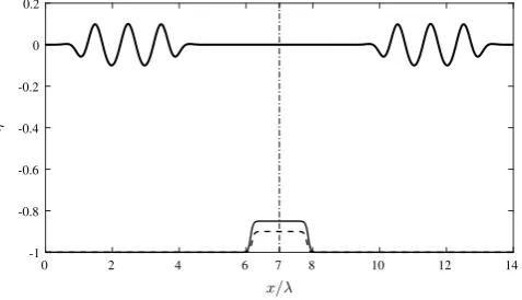
2 rule, and applied sequentially after every nonlinear operation. Time integration is handled via an optimal adaptive ordinary differential equation solver, again to the standard of common software packages (for reference, we use MATLAB).

Fig. 1.Initial configuration of numerical simulation. Thick line: Initial free surface. Thinner lines: bathymetry profile, withS=0.10 (dashed line) andS=0.15 (solid line). The dashed vertical line indicates the ‘‘barrier’’, across which mirror symmetry is imposed. Here, the wave packet’s initial wave amplitude isa0=0.10. Horizontal coordinatexis normalised by initial packet wavelengthλ0.

Mirror symmetry about the centreline of the computational domain is enforced on the initial condition, resulting in two wave packets of equal amplitude and opposite direction, starting from opposite ends of the wave tank, colliding head-on at the centre. In the absence of viscosity and surface tension, this is identical to the presence of a rigid vertical barrier [11–13]. Thus we emulate wave reflection from the vertical barrier by simulating two identical waves colliding. To clarify, the physical domain can be thought of as 0

≤

x

≤

L, the computational domain is 0

≤

x

≤

2L, and the ‘‘barrier’’ is located atx

=

L.

The free surface y

˜

0(x)

=

ζ

0(x) and the associated velocity potential

φ

˜

0(x) have the following initial conditions:

˜

y0(x)

=

W(x)a0sin [k0(x

−

x0)]

,

(27)

˜

φ

0(x)

= −

W(x)a0

ω

0

gk0

coth(k0h) cos [k0(x

−

x0)]

,

(28)

where

ω

0is the initial frequency, satisfying the finite-depth dis-persion relation

ω

2

0

=

gk0tanh(k0h)

,

(29)

andW(x) is the envelope function, satisfying

W(x)

=

1

2

[

tanh

(

x

−

x0

δ

)

−

tanh

(

x

−

x0

−

3

λ

0

δ

)]

.

(30)

This particular envelope function produces an initial wave packet containing three full wavelengths, and the initial (dimensionless) wavelength is set as

λ

0

=

125. The parameter determining the location of the initial wave packetx0is fixed at one wavelength. Additionally,

δ

≈

0

.

3

λ

0is the thickness parameter, set as such to minimise the formation of secondary waves in the early time evolution. These conditions are chosen such as to produce near optimal run-up, see Ref. [4]. The bathymetry profile considered is given by

b(x)

= −

h

+

S

2

[

tanh

(

x

−

x1

δ

s

)

−

tanh

(

x2

−

x

δ

s

)]

,

(31)

which produces a smooth ramp followed by flat ‘‘step’’. Here,his the flat ground level, set equal to one,Sis the ‘‘step height’’, and

δ

sis another thickness parameter which we set equal to L

/

100, such that in conjunction with the step edge coordinatesx1andx2, produces a ‘‘step length’’ of approximately one wavelength. The domain and set up is depicted inFig. 1. Simulations are typically performed using 215_{(32768) dealiased Fourier modes.}

[image:5.595.111.475.53.208.2]

272 J. Brennan et al. / Theoretical & Applied Mechanics Letters 7 (2017) 269–275

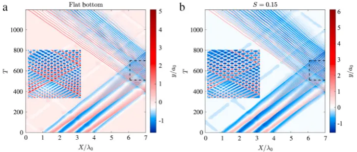
[image:5.595.124.463.263.402.2]

Fig. 2.Space time evolution of wave packet, for (a) flat bottom case and (b) step heightS=0.15 case. Free surface elevation is normalised by initial dimensionless amplitude. The inset in each panel is a zoomed in snapshot of the regions enclosed by the dashed black lines. Note the differing colour scales used, corresponding to the differing run-up amplitudes found in each case. (For interpretation of the references to colour in this figure legend, the reader is referred to the web version of this article.)

Fig. 3.(a) Run-up measured at wall. (b) Corresponding pressure load on wall. Thick grey lines: Flat bottom case, dashed lines:S= 0.10 case, thin black lines:S= 0.15 case. Note that with a stepped bathymetric profile, there is an increased shoaling effect and run-up amplitude, and conversely, reduced pressure load on wall. The effect is enhanced with increased step height.

bathymetry b(x) needs to be updated at each time step before any computations of the evolution equations can be performed. Further details may be found in Ref. [5]. We utilise a fixed point iteration scheme to updateB(

ξ,

t) from the previous time step’s estimate, with the termination condition being that the residue

R(n+1)

= ∥

H(n+1)

−

H(n)

∥

∞has decreased below a fixed tolerance

τ

R. The nature of the iteration scheme means that although the physical bathymetry profiles are prescribed to have a step length of one wavelength, this is not exactly guaranteed, and thus we refer to it as an approximate measurement.

Initially, we examine the effect of varying the step height in the bottom profile. Two step heights are chosen.S

=

0

.

10 andS

=

0

.

15, and are compared with the flat bottom case. The wave packet has an initial amplitudea0

=

0

.

1, this value being the interim amplitude examined in Ref. [6]. Time evolution of the wave packet is initially governed by shallow water dynamics, developing sharp wave fronts under the effects of nonlinear steepening. The step bathymetry amplifies this phenomenon. Eventually, dispersive ef-fects regularise the sharp fronts, generating modulated undular bores. Furthermore, enhancement of wave amplification and run-up follows as the waves meet the wall. These features are presented inFig. 2, which also compares the space time evolution of the flat bottom case andS

=

0

.

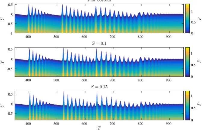
15 case.

The lower panel ofFig. 3displays the total pressure loads on the wall for each case. The increase in step height is followed by an alleviation of total pressure. This is examined in more detail in Fig. 4, which shows, in addition to total pressure, the hydrostatic and dynamic components, as well as associated power spectra. A

more detailed description of the dynamics of run-up amplification and wave evolution in this scenario can be found in Refs. [3] and [4]. Additionally, similar bore formation can be seen in the recent works of Trillo et al. [14] and Brühl et al. [15], linked with the soliton solutions of the Korteweg–de Vries equation.

Increasing the step height increases the maximum run-up, from

R

/

a0

=

5

.

23 for the flat case, toR

/

a0

=

6

.

71 for the max-imum step height considered. In each case, the maxmax-imum run-up peak is featured in the second run-run-up packet. There is also a noticeable shoaling effect, which is enhanced with larger step heights. These features can be seen clearly in the upper panel of Fig. 3.

The lower panel ofFig. 3displays the total pressure loads on the wall for each case. The increase in step height is followed by an alleviation of total pressure. This is examined in more detail in Fig. 4, which shows, in addition to total pressure, the hydrostatic and dynamic components, as well as associated power spectra. The hydrostatic contribution is approximated byPH

= −

g(y

−

[image:6.595.108.501.55.274.2] [image:6.595.137.472.327.464.2]

Fig. 4. (a)–(c) Break down of pressure components, (d)–(f) pressure spectra. Blue lines: hydrostatic pressure, red lines: total pressure, green lines: dynamic pressure. The dynamic contribution to pressure is increased with increasing bathymetric step height. Note that for increased dynamic pressure (reduced total pressure), kinks begin to appear in the pressure peaks associated to maximum run-up, a result of pressure minima forming beneath increasingly steep wave crests. (For interpretation of the references to colour in this figure legend, the reader is referred to the web version of this article.)

Fig. 5. Close up plot of the pressure ‘‘kinks’’ from simulation with step heightS=0.15, from the bottom panel ofFig. 4. Blue line: hydrostatic pressure, red line: total pressure. (For interpretation of the references to colour in this figure legend, the reader is referred to the web version of this article.)

[image:6.595.135.471.504.722.2]

274 J. Brennan et al. / Theoretical & Applied Mechanics Letters 7 (2017) 269–275

0 200 400 600 800 1000 1200 0 200 400 600 800 1000 1200

-10-20 ×10-5

-100 -10-5 -10-10 -10-15 1.2

0.8

0.6

0.4

0.2

[image:7.595.119.469.53.201.2]

0 1

Fig. 7.(a) RelativeL2error on total pressure, compared between simulations ran using 214and 215Fourier modes, forS=0.15 case. (b) Energy variation for each case. Thick grey line: flat bathymetry, dashed line:S=0.10, black line:S=0.15. Presence of step bathymetry leads to increased energy loss as waves meet vertical barrier.

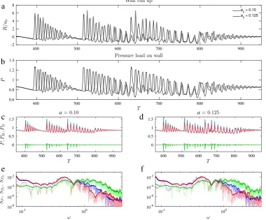
Fig. 8.Examining the effect of varying initial amplitude. Two initial amplitudes,a0=0.10 anda0=0.125, are chosen. The step height is kept constant atS=0.15. Colour coding as before. (a) Run-up compared between both cases. (b) Total pressure load on wall, for both cases. The appearance of the pressure ‘‘kinks", associated with large run-up peaks, is yet again present. (c)–(f) Comparison between hydrostatic and dynamic pressure components for (c, e)a0=0.1 and (d, f)a0=0.125 cases. Note that by increasing the initial amplitude of the wave packet, similar effects to those induced by increased step height are observed.

of the wave, which creates a pressure minima beneath the wave crest. Examining the power spectrum in Fig. 4, the increasing contribution from dynamic pressure is seen in the high-frequency domain, coinciding with the drop in total pressure compared to the hydrostatic approximation. Interestingly, further into the high-frequency region of the spectrum, the total component briefly overtakes the hydrostatic, at which point the dynamic contribution steadily decreases also, and this effect is diminished with increas-ing step height. The full pressure fields underneath the wave run-up for each case is shown inFig. 6, where the reduction in total pressure as a result of increasing step height can be seen.

[image:7.595.106.487.246.561.2]

Finally,Fig. 8displays a comparison between simulation results from two different initial amplitudes. The bathymetry profile is the same in both, using step heightS

=

0

.

15, and the two initial amplitudes area0

=

0

.

1 anda0

=

0

.

125. As can be seen, after the first wave group hits the wall, the run-up for the lower initial amplitude case is actually larger. This is likely related to optimal run-up conditions in the presence of a varying bottom, and is not thoroughly examined in this work. The converse is true for the pressure load, which is larger for the increased amplitude case. Although the run-up is slightly smaller for increased amplitude, the waves themselves are still larger, and as such, the pressure is too. Finally, for the increased amplitude case, the largest run-up is now found in the leading run-up packet. As such, the pressure ‘‘kinks’’ are present again, however given the largest run-up peak is now in the leading packet, the kink is now positioned as such.

In conclusion, we have presented an examination of extreme wave run-up on a vertical wall, in the presence of a varying bathymetry, and in addition, the associated pressure fluctuations are computed. This investigation is facilitated by Euler equation numerical simulations based on the conformal mapping method. The procedure used to identify the pressure field beneath the free surface is also described.

An increasing bottom profile enhances already extreme wave run-up, but decreases the associated pressure load, which is over-estimated by the hydrostatic approximation. As such, the dynamic pressure contribution is amplified by the rising sea bed. In terms of the pressure spectrum, this increased dynamic component is seen in the high-frequency region. Increasing the amplitude of the initial wave packet also enhances this phenomenon. The pressure peaks associated with the largest run-up feature the most striking dynamical component, giving rise to the formation of ‘‘kinks’’ in the peaks.

We note that this is a simple investigation, in which we have highlighted the potential effect the varying bottom profile has. A wide class of profiles can be considered, providing scope for future work. The wave parameters considered in this work were chosen to provide near optimal run-up, of which a detailed description can be found in Refs. [3,4]. Optimal conditions in the presence of varying bathymetry have not yet been determined.

As mentioned in Ref. [6], aside from this works relevance to maritime engineering, there is also an interesting implication to microseisms. Longuet–Higgins [16] work on microseisms provided a basis for research on the influence of nonlinear waves on seismic noise, and it is still an active topic today [17,18]. Pressure fluctu-ations on the sea bed associated with the run-up of long waves contain a considerable high-frequency component in their power spectrum, similar to the typical frequency band associated with microseisms.

A further potential application of this work is in the inves-tigation of boulder-sized deposits along exposed coastlines. The movement of such large masses indicates that the affected coasts experience extremely high-energy wave events (for example, see Cox et al. [19]). Recent research [19,20] focussed on the west coast of Ireland has shown that storm waves, rather than tsunamis, are capable of producing such movements, despite calculations indicating that this should not be possible [21]. This suggests that fully-nonlinear wave models, with the resulting extreme run-up

and pressure loads discussed in this present work, are needed to completely understand these phenomena.

Acknowledgements

This work is supported by the European Research Coun-cil (ERC) under the research project ERC-2011-AdG 290562-MULTIWAVE, the Science Foundation Ireland (SFI) under grant number SFI/12/ERC/E2227, and also under the research project ‘‘Understanding Extreme Nearshore Wave Events through Studies of Coastal Boulder Transport’’ funded through the US-Ireland R & D Programme (14/US/E3111 and NSF 1529756). The authors would like to thank James Herterich for fruitful discussion on the topic.

References

[1] L. O’Brien, J.M. Dudley, F. Dias, Extreme wave events in Ireland, Nat. Hazards Earth Syst. Sci. 13 (2013) 625–648.

[2] D.H. Peregrine, Water-wave impact on walls, Annu. Rev. Fluid Mech. 35 (2003) 23–43.

[3] F. Carbone, D. Dutykh, J.M. Dudley, et al., Extreme wave run-up on a vertical cliff, Geophys. Res. Lett. 40 (2013) 3138–3143.

[4] C. Viotti, F. Carbone, F. Dias, Conditions for extreme wave run-up on a vertical barrier by nonlinear dispersion, J. Fluid Mech. 748 (2014) 768–788.

[5] C. Viotti, D. Dutykh, J.M. Dudley, et al., The conformal mapping method for sur-face gravity waves in the presence of variable bathymetry and mean current, Proc. IUTAM 11 (2014) 110–118.

[6] J. Brennan, C. Viotti, F. Dias, Pressure fluctuations on a vertical wall during ex-treme run-up cycles, J. Offshore Mech. Arctic Eng. OMA E2014–23444 (2014).

[7] G. Akrish, R. Schwartz, O. Rabinovitch, et al., Impact of extreme waves on a vertical wall, Nat. Hazards 84 (2016) 637–653.

[8] G. Akrish, O. Rabinovitch, Y. Agnon, Extreme run-up events on a vertical wall due to nonlinear evolution of incident wave groups, J. Fluid Mech. 797 (2016) 644–664.

[9] A.L. Dyachenko, V.E. Zakharov, E.A. Kuznetsov, Nonlinear dynamics on the free surface of an ideal fluid, Plasma Phys. Rep. 22 (1996) 916–928.

[10] W. Choi, R. Camassa, Exact evolution equations for surface waves, J. Eng. Mech. 125 (1999) 756–760.

[11] J.L. Bona, W.G. Pritchard, L.R. Scott, Solitary-wave interaction, Phys. Fluids 197 (1980) 503–521.

[12] M.J. Cooker, P.D. Weidman, D.S. Bale, Refection of a high-amplitude solitary wave at a vertical wall, J. Fluid Mech. 342 (1997) 141–158.

[13] W. Craig, P. Guyenne, J. Hammack, et al., Solitary water wave interactions, Phys. Fluids 18 (2006) 57106.

[14] S. Trillo, G. Deng, G. Biondini, et al., Experimental observation and theoretical description of multisoliton fission in shallow water, Phys. Rev. Lett. 117 (2016) 144102.

[15] M. Brühl, H. Oumeraci, Analysis of long-period cosine-wave dispersion in very shallow water using nonlinear Fourier transform based on KdV equation, App. Ocean Res. 61 (2016) 81–91.

[16] M.S. Longuet-Higgins, A theory of the origin of microseisms, Phil. Trans. Roy. Soc. London A 243 (1950) 1–35.

[17] F. Ardhuin, T.H.C. Herbers, Noise generation in the solid earth, oceans and atmosphere, from nonlinear interacting surface gravity waves in finite depth, J. Fluid Mech. 716 (2013) 316–348.

[18] L. Pellet, P. Christodoulides, S. Donne, et al., Pressure induced by the interaction of water waves nearly equal frequencies and nearly opposite directions, Theor. Appl. Mech. Lett. 7 (2017) 138–144.

[19] R. Cox, D.B. Zentner, B.J. Kirchner, et al., Boulder ridges on the aran Islands (Ireland): Recent movements caused by storm waves, not tsunamis, J. Geol. 120 (2012) 249–272.

[20] D.M. Williams, A.M. Hall, Cliff-top megaclast deposits of Ireland, a record of extreme waves in the North Atlantic — storms or tsunamis? Mar. Geol. 206 (2004) 101–117.