DMGroup at EmoInt 2017: Emotion Intensity Using Ensemble Method

DMGroup at EmoInt-2017: Emotion Intensity Using Ensemble

Method

Xiaotian Han

and

Song Jiang

!

_{Department of Computer Science and Technology,}

_{Beijing University of Posts and}

Telecommunications

"

_{Department of Microelectronic,}

_{Tsinghua University}

[email protected], [email protected]

Abstract

In this paper, we present a novel ensemble learning architecture for emotion intensity analysis, particularly a novel framework of ensemble method. The ensemble method has two stages and each stage includes several single machine learning models. In stage1, we employ both linear and nonlinear regression models to obtain a more diverse emotion intensity representation. In stage2, we use two regression models including linear regression and XGBoost. The result of stage1 serves as the input of stage2, so the two different type models (linear and non-linear) in stage2 can describe the input in two opposite aspects. We also added a method for analyzing and splitting multi-words hashtags and appending them to the emotion intensity corpus before feeding it to our model. Our model achieves 0.571 Pearson-measure for the average of four emotions.

1

Introduction

Social media has evolved into a data source that is massive and growing rapidly. Analyzing the emotion of a user‘s tweet can be helpful to the tasks from personalized advertising to public health monitoring and surveillance. Emotion analysis is a warm area of Natural Language

Processing (NLP) dealing with the intensity of emotion in tweets. (An.Y, et al., 2017) Traditional emotion analysis problems are usually classification tasks such as emotion classification (Bandhakavi, et al., 2017). Some of the methods of this task usually use manually designed semantic lexicon. However, these semantic lexicons usually are not general to different corpus and targets and it will take much time to build the

semantic lexicon. And some researchers establish the models using signal machine learning algorithms such as Support Vector Machine (SVM) and naive Bayes (Tang B et al., 2016) However, such signal model just describes the corpus in only one aspect, which will lead to inaccuracy of the emotion analysis since every single model has its own disadvantages. In recent KDD CUPs, winner solutions are not signal models. (Sandulescu, et al 2016, Kadam et al 2015)

Ensemble based methods are among the most widely used techniques for data science problems. Their popularity is because of their good performance compared with strong single learners while being quite easy to arrange in real-world applications. It has been proved in many competitions such as Kaggle competitions (Zou et al 2017) and KDD CUPs mentioned above. Ensemble algorithms usually perform well in the data learning tasks as they can be integrated with different signal algorithms and the strategy of ensemble can be adjusted according to each task.

learning architecture for emotion intensity analysis, particularly a novel framework of ensemble method. Our model participated in the WASSA-2017 shared task emotion intensity analysis in tweets. (Mohammad, S.M, et al2017) The goal of the task was to automatically determine the intensity or degree of emotion X when given a tweet and an emotion X. We treat this task as a regression problem. Our ensemble method includes two stages and each stage includes several single regression models. The method can obtain a diverse emotion intensity representation of the corpus. In stage1, we employ three models containing both linear and non-linear regression models and the result of stage1 serves as the input of the stage2. Stage2 has two regression models including linear regression and XGBoost. And finally, the results of the two models in stage2 are added with weights. Meanwhile, we analyze and split multi-words hashtags and this result is also in the algorithm. Our average Pearson-measure score for the average of four emotions is 0.571(shown in Table7).

2

Related Work

A large amount of work related to analyzing emotion have been done. A very broad overview of the existing work was presented in (Pang and Lee, 2008). Meanwhile, there are lots of related work using deeply models (Majumder et al, 2017). In their survey, the authors described existing techniques and approaches for the sentiment analysis and information retrieval. In the paper (Pang et al. 2002) which used machine learning models to predict sentiments in text, the approach showed that SVM classifiers trained using bag-of-words features produced hopeful results. In the paper (Yang et al., 2007), the authors used emotion icons in the blog posts as significant indicators of users sentiment. The authors applied SVM classifier to classify sentiments at the sentence level and then study the overall sentiment of the document. However, social media sources, such as Twitter posts, presented many unsolved natural language processing (NLP) tasks and machine learning challenges. As the intensive study of machine learning in the NLP task, some of the key challenges including data imbalance, noise, and feature sparseness may be solved.

3

System Description

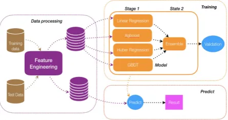
Fig 1 shows the architecture of our ensemble learning model. The core framework of our ensemble models includes the two stages. The ensemble model is an improved version of stacking (Wolpert, 1992; Zhou, 2012). After data processing and feature engineering, the features are sent to the stage1. We test various kinds of regression models. Finally, we find the four regression models can achieve satisfying performance on these features. (Table 6) In stage1, including Linear Regression, Huber Regression, Gradient Boost Decision Trees and XGBoost. The former two models are linear models and the latter two are non-linear. The output of the two different models will be gotten by linear and non-linear algorithms based on raw features, which guarantees the diverse representation of the raw features. With the output of stage1 serves as the input, stage2 also has both linear and non-linear models, including Huber Regression and XGBoost, which are covered by Ensemble block in the figure1.According to the characteristics of data, we carefully tune these models and find some tricks (such as ‘emoji’ expression) to achieve better performance than raw data. The tuning work will be discussed in following single model sections.

3.1 XGBoost

XGBoost (Chen, T et al,2016) is an open-source software library which provides the gradient boosting framework. From the project description, it aims to provide a Scalable, Portable and Distributed Gradient Boosting (GBM, GBRT, GBDT) Library. In this work, we use XGBoost to as one of the four signal models of stage1 and ensemble model in stage2.

XGBoost has gained much popularity and attention recently as it was the algorithm of choice for many winning teams of a number of machine learning competitions. For example, in all the 29 winning solutions published at Kaggle’s blog during 2015, 17 teams used XGBoost.

3.2 Gradient Boosting Decision Tree

Gradient Boosting Decision Tree (GBDT) uses decision trees as base learners and combines them into a single strong learner. (Drucker,1996) The final prediction of GBDT is the weighted sum of outputs from each tree. In Stage 1, the model is implemented by scikit-learn package (Pedregosa.F et al, 2011). There are some specific parameters in GBDT: the number of trees (iterations), learning rate, the maximum depth of each tree and the minimum number of samples in a leaf. The last two parameters control the size of each tree. Empirical results show that small values of learning rate favor better test error (Zeiler et al 2012), so we set it as 0.03 in both Stage 1. In Stage 1, we train 500 trees with no less than 50 samples in each leaf, since the data set is much larger.

3.3 Linear Regression

We use the implementation of regularized linear regression from scikit-learn (Pedregosa, F et al 2011) package, with liblinear library solver, to train learner. L2 regularization is chosen to avoid overfitting. We have done tuning work in the training dataset and tried to find the best set of parameters. Finally, the regularization strength is set to 50. Since the distribution of labels in training dataset is not uniform just like class imbalance in classification problem, the weight of positive samples is set to 100, while the weight of negative samples is 1. In addition, the values of all features are normalized to the range of [0,1] with the minimum-maximum scaler.

3.4 Huber Regression

The Huber Regressor (Jeng J et al 2009)optimizes the squared loss for the samples where |(y −

X0_{w)/sigma| < epsilon and the absolute loss for the}

samples where |(y −X0_{w)/sigma| > epsilon, where}

w and sigma are parameters to be optimized. In Huber Regression, the parameter sigma is an adjustment factor to guarantee the robustness. In other word, if y is scaled up or down by a certain factor, we do not need to rescale the epsilon. The

model we trained to achieve the best average Pearson-measure score 0.554.

4

Feature Engineering

4.1 Data Processing and Feature Extraction All the data used for training the emotion intensity regression model undergoes the following preprocessing algorithm. Firstly, to determine the importance of word in an emotion, we use a tokenize to separate the corpus into a series of single word. The TfidfVectorizer in the open source sickit-learning (Sklearn) is used to complete this. Secondly, the URL text and other useless specific symbols such as ‘/’ and ‘_’ should be removed from the features because this type of text may mislead the regression model. Then the context information is supposed to be considered since a word may not cover enough information in short texts. Finally consider the following two tweet, “Sometimes I get mad over something so minuscule I try to ruin somebodies life not like lose your job like get you into federal prison”and “Sometimes I get mad over something so minuscule I try to ruin somebodies life not like lose your job like get you into federal prison #anger “. The two tweets are nearly same except the last expression tags #anger, which leads to a different intensity. However, the symbol # is removed by TfidfVectorizer, and so is emoji expressions. As a result, these expression texts should be added into the features. Totally, the raw data is processed to features in following steps:

1. Using Scikit-learn TfidfVectorizer to tokenize each tweet.

2. Remove the useless text data including URL and specific symbol.

emotions train numbers dev numbers

anger 857 84

sadness 786 74

joy 823 110

fear 1147 110

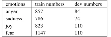
Table 1: The numbers of instances training dataset and dev datasets

4. Since default model TfidfVectorizer will remove the emoji and tweet tags, these key expressions need to be recalled.

4.2 Feature Selection

The number of features for the four emotions is from 3722 to 3945 by methods of feature extraction mentioned above. However, some of them are redundant. To improve the efficiency, we design a feature selection strategy to further select the features. Specifically, to avoid overfitting and remove useless features, we design three different

Table 2: anger’s words analysis

validation sets (each one 10% of training dataset) and make sure that each feature has performance improvement on all of three validation sets, and then we choose it as an effective feature. This selection process is very important because we can detect if a feature is useful. Finally, 3010 features out of more than 3722 are obtained.

5

Experiments and Analysis

To train and validate our models for this task, we used the dataset provided for Shared Task on Emotion Intensity. (Mohammad, S.M, et al2017)

We obtained 857 instances from the training datasets and 84 instances from the Development datasets for the anger intensity, and others show in Table1.We build four different models for the four Emotions: anger, sadness, joy and fear. Table 1 shows the distribution of datasets about all subtasks. All the experiments have been developed using scikit-learn. The models were trained using the default parameters. All our experiments were performed on a machine with Intel Core i5 CPU @ 2.00GHz (4 cores), 8GB of RAM.

5.1 Four Emotion Models

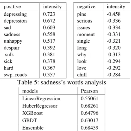
The single model with best score is Huber Regressor, which gets the Pearson of 0.682 in

anger task. In the training process of Huber Regressor, every word gets a score of intensity of anger. For example, the word “fucking” gets the 0.609, which is the highest score of intensity of

positive intensity negative intensity nervous panic anxiety nightmare die shudder scared gonna comments cry 0.883 0.852 0.789 0.670 0.524 0.514 0.470 0.462 0.449 0.442 terrific excited refuse wrong love serious year walking yes kissed -0.446 -0.334 -0.320 -0.318 -0.313 -0.308 -0.303 -0.300 -0.299 -0.295

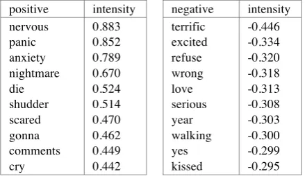
Table 3: fear’s words analysis

anger. In fact, the word “fucking” mostly means anger. So, the model can represent the intensity of the emotion precisely. Table 2,3,4,5 show the top positive and negative words in four subtasks. As the tables show, the words in the table can reflect the intensity of each emotions.

Table 6 shows our results of the four models on the development datasets for anger emotion intensity prediction. The other three emotions` results are similar to this (not listed here).

5.2 Ensemble Results

Table 7 shows our results on the development datasets and the test datasets for all four subtasks. According to the scores and our ranking in leaderboard, we noticed that our model was not as we expected, which might mainly due to the following reasons:

1. Recently most of teams in many

competitions use Neural Networks. As we know, deep learning needs plentiful training dataset(Goodfellow,2016).

positive intensity negative intensity hilarious laughter thanks happy gets myahris.. meant lol exhilar.. nick_off.. 0.612 0.461 0.444 0.428 0.426 0.423 0.420 0.414 0.406 0.372 pity hate barmy.. tears bit fucking sad say last stop -0.458 -0.448 -0.420 -0.383 -0.382 -0.379 -0.365 -0.335 -0.327 -0.319

Table 4: joy’s words analysis

positive intensity negative intensity depressing

depression sad sadness unhappy despair sulk sick hard swp_roads

0.723 0.672 0.603 0.558 0.517 0.392 0.381 0.378 0.367 0.357

pine serious issues moment single long why look love chill

-0.458 -0.336 -0.334 -0.331 -0.321 -0.320 -0.313 -0.294 -0.292 -0.284

Table 5: sadness’s words analysis

models Pearson

LinearRegression 0.55061 HuberRegressor 0.68261

XGBoost 0.64796

GBDT 0.63017

Ensemble 0.68459

Table 6: results of different models of anger

However, our model did not use the Neural Networks and Word Embedding, because the number of training data is not abundant, but we will have try to apply the neural network method to this task in the future.

2. We did not use grid-search to find the best set of parameters of each single model. So, our model can be improved. And we did not use complicated ensemble methods compared with ensemble methods described in (Dietterich, 2002).

3. We did not use the extra information of the emotion intensity of every word which means that we learning the emotion intensity just from the datasets provided. The training datasets and development datasets all the information that we used in the task.

Although our model has a gap with the top teams, we have some advantages as following:

1. we did not consume excessive computing resources, and our training time is ms-level which is fast enough for this task. And our model is suitable for all the subtask while all the subtask has the same model and all the emotions intensity predicted is stable enough, which is robust in train set, development set and test set.

2. After training, we can obtain an extra emotion lexicon which can be used for other

Unsupervised learning task, such as obtain a unlabeled sentence emotion intensity as the scores of four subtask in dev and test datasets have no big difference.

emotions dev Pearson test Pearson

anger 0.68459 0.550

sadness 0.47009 0.603

joy 0.66913 0.556

fear 0.56406 0.576

average 0.59697 0.571

Table 7: The results of dev datasets and test datasets (5% lower than baseline)

6

Conclusion and Further Work

Our model achieved moderate performance on the emotion intensity sentiment analysis task with very basic settings include the default setting of the parameters of the methods. Considering that the performance of our model was achieved by a sample settings, there is big achievement of better performance by adopting the more exquisite methods and the more feature engineering. We have several planned works to improve the performance in this task, including the more fusion of the methods and the statistical feature. We will also attempt to optimize our models further and use the word embedding which may provide additional information to improve our performance.

Acknowledgments

We would like to acknowledge the support of the Beijing University of Posts and

Telecommunications and Tsinghua University.

References

An, Y., Sun, S., & Wang, S. 2017. Naive Bayes classifiers for music emotion classification based on lyrics. In Computer and Information Science (ICIS), 2017 IEEE/ACIS 16th International Conference on (pp. 635-638). IEEE.

Bandhakavi, A., Wiratunga, N., Padmanabhan, D., & Massie, S. 2017. Lexicon based feature extraction for emotion text classification. Pattern Recognition Letters, 93, 133-142.

Tang, B, Kay, S., & He, H. 2016. Toward optimal feature selection in naive bayes for text categorization. IEEE Transactions on Knowledge & Data Engineering, 28(9), 2508-

2521.

Kadam, Priti, et al. 2015."KDD CUP 2015-Predicting Dropouts in MOOC’S." Imperial Journal of Interdisciplinary Research 2(5).

Zou, Haosheng, Kun Xu, and Jialian Li. 2017 "The YouTube-8M Kaggle Competition: Challenges and Methods." arXiv preprint arXiv:1706.09274.

Mohammad, Saif M. and Bravo-Marquez, Felipe. September 2017. "WASSA-2017 Shared Task on Emotion Intensity". In Proceedings of the EMNLP 2017 Workshop on Computational Approaches to Subjectivity, Sentiment, and Social Media (WASSA) Copenhagen, Denmark.

Pang, Bo, Lee, & Lillian. 2008. Opinion mining and sentiment analysis. Foundations & Trends

in Information Retrieval, 2(1–2), 1-135.

Majumder, N., Poria, S., Gelbukh, A., & Cambria, E. 2017. Deep Learning-Based Document Modeling for Personality Detection from Text. IEEE Intelligent Systems, 32(2), 74-79.

Pang, B., Lee, L., & Vaithyanathan, S. July 2002,. Thumbs up?: sentiment classification using machine learning techniques.

In Proceedings of the ACL-02 conference on Empirical methods in natural language

processing-Volume 10 (pp. 79-86). Association for Computational Linguistics. Yang, C., Lin, K. H. Y., & Chen, H. H. November 2007. Emotion classification using web blog corpora. In Web Intelligence, IEEE/WIC/ACM International Conference on (pp. 275-278). IEEE.

Wolpert, D. H. 1992. Stacked generalization .Neural networks, 5(2), 241-259.

Zhou, Z. H. 2012. Ensemble methods: foundations and algorithms. CRC press. Chen, T., & Guestrin, C. August 2016.

Xgboost: A scalable tree boosting system. In Proceedings of the 22Nd ACM SIGKDD International Conference on Knowledge Discovery and Data Mining (pp. 785-794). ACM.

Drucker, H., & Cortes, C. 1996. Boosting decision trees. In Advances in neural information processing systems (pp. 479-485).

Pedregosa, F., Varoquaux, G., Gramfort, A., Michel, V., Thirion, B., Grisel, O., ... & Vanderplas, J. 2011. Scikit-learn: Machine learning in Python. Journal of Machine Learning Research, 12(Oct), 2825-2830.

Zeiler, M. D. 2012. ADADELTA: an adaptive learning rate method. arXiv preprint arXiv:1212.5701.

Jeng, J. H., Tseng, C. C., & Hsieh, J. G. 2009. Study on Huber fractal image compression. IEEE Transactions on Image Processing,18(5), 995- 1003.

Pedregosa, F., Varoquaux, G., Gramfort, A., Michel, V., Thirion, B., Grisel, O., ... & Vanderplas, J. (2011). Scikit-learn: Machine learning in Python. Journal of Machine

Learning Research, 12(Oct), 2825-2830. Brown, P. F., Desouza, P. V., Mercer, R. L.,

Pietra, V. J. D., & Lai, J. C. 1992. Class- based n-gram models of natural language Computational linguistics, 18(4), 467-479.

Goodfellow, I., Bengio, Y., & Courville, A. 2016. Deep learning. MIT press.