Proceedings of the Twelfth Workshop on Graph-Based Methods for Natural Language Processing (TextGraphs-12), pages 7–11
Efficient Generation and Processing of Word Co-occurrence Networks
Using corpus2graph
Zheng ZhangLIMSI, CNRS, Universit´e Paris-Saclay
Orsay, France
LRI, Univ. Paris-Sud, CNRS, Universit´e Paris-Saclay
Orsay, France
Ruiqing Yin LIMSI, CNRS, Universit´e Paris-Saclay
Orsay, France
Pierre Zweigenbaum LIMSI, CNRS, Universit´e Paris-Saclay
Orsay, France [email protected]
Abstract
Corpus2graph is an open-source NLP-application-oriented Python package that generates a word co-occurrence network from a large corpus. It not only contains different built-in methods to preprocess words, analyze sentences, extract word pairs and define edge weights, but also supports user-customized functions. By using paral-lelization techniques, it can generate a large word co-occurrence network of the whole English Wikipedia data within hours. And thanks to its nodes-edges-weight three-level progressive calculation design, rebuilding networks with different configurations is even faster as it does not need to start all over again. This tool also works with other graph libraries such as igraph, NetworkX and graph-tool as a front end providing data to boost network generation speed.
1 Introduction
Word co-occurrence networks are widely used in graph-based natural language processing methods and applications, such as keyword extraction (Mi-halcea and Tarau,2004) and word sense discrimi-nation (Ferret,2004).
A word co-occurrence network is a graph of word interactions representing the co-occurrence of words in a corpus. An edge can be created when two words co-occur within a sentence; these words are possibly non-adjacent, with a maximum distance (in number of words, see Section 2.2) defined by a parameter dmax (Cancho and Sol´e,
2001). In an alternate definition, an edge can be created when two words co-occur in a fixed-sized sliding window moving along the entire document or sentences (Rousseau and Vazirgiannis, 2013). Despite different methods of forming edges, the structure of the network for sentences will be the same for the two above definitions if the maximum
distance of the former is equal to the sliding win-dow size of the latter. Edges can be weighted or not. An edge’s weight indicates the strength of the connection between two words, which is often related to their number of co-occurrences and/or their distance in the text. Edges can be directed or undirected (Mihalcea and Radev,2011).
While there already exist network analysis packages such as NetworkX (Hagberg et al., 2008), igraph (Csardi and Nepusz, 2006) and graph-tool (Peixoto, 2014), they do not include components to make them applicable to texts di-rectly: users have to provide their own word preprocessor, sentence analyzer, weight function. Moreover, for certain graph-based NLP applica-tions, it is not straightforward to find the best net-work configurations, e.g. the maximum distance between words. A huge number of experiments with different network configurations is inevitable, typically rebuilding the network from scratch for each new configuration. It is easy to build a word co-occurrence network from texts by using tools like textexture1 or GoWvis2. But they mainly fo-cus on network visualization and cannot handle large corpora such as the English Wikipedia.
Our contributions: To address these incon-veniences of generating a word co-occurrence network from a large corpus for NLP applica-tions, we propose corpus2graph, an open-source3 NLP-oriented Python package designed to handle Wikipedia-level large corpora. Corpus2graph sup-ports many language processing configurations, from word preprocessing to sentence analysis, and different ways of defining network edges and edge attributes. By using our node-edge-weight three-level progressive calculation design, it can quickly build networks for multiple configurations.
1http://textexture.com
2https://safetyapp.shinyapps.io/GoWvis/
3available at https://github.com/zzcoolj/corpus2graph
We are currently using it to experiment with injecting pre-computed word co-occurrence net-works into word2vec word embedding computa-tion.
2 Efficient NLP-oriented graph generation
Our tool builds a word co-occurrence network given a source corpus and a maximal distance dmax. It contains three major parts: word
process-ing, sentence analysis and word pair analysis from an NLP point of view. They correspond to three different stages in network construction.
2.1 Node level: word preprocessing
The contents of large corpora such as the whole English Wikipedia are often stored in thousands of files, where each file may contain several Wikipedia articles. To process a corpus, we con-sider a file as the minimal processing unit. We go through all the files in a multiprocessing way: Files are equally distributed to all processors and each processor handles one file at a time.
To reduce space requirements, we encode each file by replacing words with numeric ids. Be-sides, to enable independent, parallel processing of each file, these numeric ids are local to each process, hence to each file. A local-id-encoded file and its corresponding local dictionary (word →local id) are created after this process. As this process focuses on words, our tool provides sev-eral word preprocessing options such as tokenizer selection, stemmer selection, removing numbers and removing punctuation marks. It also supports user-provided word preprocessing functions.
All these local-id-encoded files and correspond-ing local dictionaries are stored in a specific folder (dicts and encoded texts). Once all source files are processed, a global dictionary (word→global id) is created by merging all local dictionaries. Note that at this point, files are still encoded with local word ids.
2.2 Node co-occurrences: sentence analysis
To prepare the construction of network edges, this step aims to enumerate word co-occurrences, tak-ing into account word distance. Given two words wi
1 andw2j that co-occur within a sentence at po-sitions i and j (i, j ∈ {1. . . l} where l is the number of words in the sentence), we define their distance d(wi
1, wj2) = j − i . For each input
δ Word Pairs
2 (8746, 2357), (2357, 2669), (2669, 4), (4, 309), (309, 1285), (1285, 7360)
3 (8746, 2669), (2357, 4), (2669, 309), (4, 1285), (309, 7360)
[image:2.595.315.520.60.135.2]4 (8746, 4), (2357, 309), (2669, 1285), (4, 7360) 5 (8746, 309), (2357, 1285), (2669, 7360)
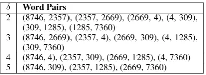
Table 1: Word pairs for different values of distanceδ in sentence “8746 2357 2669 4 309 1285 7360”
file, dmax output files will be created to
enumer-ate co-occurrences: one for each distance δ ∈ {1, . . . dmax}. They are stored in thecoocfolder.
To prepare the aggregation of individual statis-tics into global statisstatis-tics (see Section 2.3), each process converts local word ids into global word ids through the combination of its local dictionary and of the global dictionary. Note that at this point the global dictionary must be loaded into RAM.
Then, a sentence analyzer goes through this file sentence by sentence to extract all word co-occurrences with distances δ ≤ dmax. For
in-stance, sentence “The NLP history started in the 1950s.” may be encoded as “8746 2357 2669 4 309 1285 7360”; the sentence analyzer will extract word pairs from distance 1 todmax. The results for
dmax = 5are shown in Table1.
User-customized sentence analyzer and dis-tance computation are also supported so that more sophisticated definitions of word pair distance can be introduced. For instance, we plan to provide a syntactic distance: the sentence analyzer will build a parse tree for each sentence and compute word pair distance as their distance in the parse tree.
Besides, in this step, we also provide an option to count the number of occurrences of each word occ(w). Given that a large corpus like Wikipedia
has a huge number of tokens, a global word count is convenient to enable the user to select words based on a frequency threshold before network generation. We return to this point in the next sub-section.
2.3 Edge attribute level: word pair analysis
A word pair (w1, w2) is represented by an edge linking two nodes in the word co-occurrence net-work. In this step, we enrich edge information withdirectionandweightby word pair analysis.
co-occurrences of w1 and w2 with distances δ≤dmax(Eq.2).
cooc(δ, w1, w2) =|{(wi1, w2j);d(wi1, wj2) =δ}| (1)
w(dmax, w1, w2) =
X
δ≤dmax
cooc(δ, w1, w2) (2)
For efficiency we use an iterative algorithm (Eq.3):
w(d, w1, w2) =
cooc(1, w1, w2), ifd= 1 cooc(d, w1, w2)+
w(d−1, w1, w2), otherwise (3)
We calculate the edge weight of different window sizes in a stepwise fashion by applying Eq.3. For the initial calculation, we start by counting and merging all word pair files of distance 1 in the
edges folder generated by step 2 to get a co-occurrence count file. This file contains informa-tion on all distinct word pair co-occurrence counts for distance 1. We then follow the same principle to obtain a co-occurrence count file for distance 2. We merge this result with the previous one to get word pair co-occurrence counts for window size 2. We continue this way until distancedmax.
If we wish to make further experiments with a larger distance, there is no need to recompute counts from the very beginning: we just need to pick up the word pair co-occurrences of the largest distance that we already calculated and start from there. All co-occurrence count files for the differ-ent distances are stored in thegraphfolder.
Defining the weight as the sum of co-occurrences of two words with different distances is just one of the most common ways used in graph-based natural language processing applica-tions. We also support other (built-in and user-defined) definitions of the weight. For instance, when calculating the sum of co-occurrences, we can assign different weights to co-occurrences ac-cording to the word pair distance, to make the re-sulting edge weight more sensitive to the word pair distance information.
For a large corpus, we may not need all edges to generate the final network. Based on the word count information from Section 2.2, we may se-lect those nodes whose total frequency is greater than or equal to min count, or the most frequent
vocab sizenumber of nodes, or apply both of these constraints, before building edges and computing their weights.
3 Efficient graph processing
3.1 Matrix-type representations
Although our tool works with graph libraries like igraph, NetworkX and graph-tool as a front end, we also provide our own version of graph pro-cessing class for efficiency reasons: Most graph libraries treat graph processing problems in a net-work way. Their algorithms are mainly based on network concepts such as node, edge, weight, de-gree. Sometimes, using these concepts directly in network algorithms is intuitive but not computa-tionally efficient. As networks and matrices are interchangeable, our graph processing class uses matrix-type representations and tries to adapt net-work algorithms in a matrix calculation fashion, which boosts up the calculation speed.
In our matrix representation for graph informa-tion, nodes, edges and weights are stored in an ad-jacency matrix A: a square matrix of dimension |N| × |N|, whereN is the number of nodes in the graph. Each row of this matrix stands for a start-ing node, each column represents one endstart-ing node and each cell contains the weight of the edge from that starting node to the ending node.
Note that not all network algorithms are suit-able for adapting into a matrix version. For this reason, our graph processing class does not aim to be a replacement of the graph libraries we men-tioned before. It is just a supplement, which pro-vides matrix-based calculation versions for some of the algorithms.
To give the reader an intuition about the differ-ence between the common network-type represen-tation and the matrix-type represenrepresen-tation, the com-ing subsection uses the random walk algorithm as an example.
3.2 Random walk
Random walks (Aldous and Fill,2002) are widely used in graph-based natural language process-ing tasks, for instance word-sense disambigua-tion (Moro et al., 2014) and text summariza-tion (Erkan and Radev, 2004; Zhu et al., 2007). The core of the random walk related algorithms calculation is the transition matrixP.
In the random walk scenario, starting from an initial vertex u, we cross an edge attached to u that leads to another vertex, sayv (v can beu it-self when there exists an edge that leads fromuto u, which we call a self-loop). ElementPuvof the
prob-abilityP(u, v)of the walk from vertexuto vertex v in one step. For a weighted directed network, P(u, v)can be calculated as the ratio of the weight
of the edge(u, v) over the sum of the weights of the edges that start from vertexu.
NetworkX (version 2.0) provides a built-in
methodstochastic graphto calculate the transition matrix P. For directed graphs, it starts by cal-culating the sum of the adjacent edge weights of each node in the graph and stores all the results in memory for future usage. Then it traverses every edge(u, v), dividing its weight by the sum of the
weights of the edges that start fromu.
Based on the adjacency matrixAintroduced in Section3.1, the transition probabilityP(u, v)can
be expressed as:
P(u, v) =Auv/ |APu|
i=1 Aui
The transition matrix P can be easily calcu-lated in two steps: First, getting sums of all el-ements along each row and broadcasting the re-sults against the input matrix to preserve the di-mensions (keepdimsis set to True); Second, per-forming element-wise division to get the ratios of each cell value to the sum of all its row’s cell val-ues. By using NumPy (Walt et al.,2011), the cal-culation is more efficient both in speed and mem-ory. Besides, as the calculations are independent of each row, we can take advantage of multipro-cessing to further enhance the computing speed.
4 Experiments
4.1 Set-up
In the first experiment, we generated a word co-occurrence network for a small corpus of 7416 to-kens (one file of the English Wikipedia dump from April 2017) without using multiprocessing on a computer equipped with the Intel Core i7-6700HQ processor. Our tool serves as a front end to provide nodes and edges to the graph libraries NetworkX, igraph and graph-tool. In contrast, the baseline method processes the corpus sentence by sentence, extracting word pairs with a distance δ ≤ dmax
and adding them to the graph as edges (or updat-ing the weight of edges) through these libraries. All distinct tokens in this corpus are considered as nodes.
In the second experiment, we used our tool to extract nodes and edges for the generation of a word co-occurrence network on the entire En-glish Wikipedia dump from April 2017 using 50
logical cores on a server with 4 Intel Xeon E5-4620 processors ,dmax = 5,min count = 5and
vocab size= 10000.
In the last experiment, we compared the random walk transition matrix calculation speed on the word co-occurrence network built from the pre-vious experiment result between our method and the built-in method of NetworkX (version2.0) on
a computer equipped with Intel Core i7-6700HQ processor.
4.2 Results
NetworkX igraph graph-tool baseline 4.88 8727.49 77.70
corpus2graph 15.90 14.47 14.31
Table 2: Word network generation speed (seconds)
Table2shows that regardless of the library used to receive graph information generated by cor-pus2graph, it takes around 15 seconds from the small Wikipedia corpora to the final word co-occurrence network. And our method performs much better than the baseline method with igraph and graph-tool even without using multiprocess-ing. We found that in general loading all edges and nodes information at once is faster than load-ing edge and node information one by one and it takes approximately the same time for all graph libraries. As for NetworkX, the baseline method is faster. But as the corpora get larger, the base-line model uses more and more memory to store the continuously growing graph, and the process-ing time increases too.
For the second experiment, our tool took around
236 seconds for node processing (Section 2.1), 2501 seconds for node co-occurrence analysis
(Section2.2) and8004seconds for edge
informa-tion enriching (Secinforma-tion 2.3). In total, it took less than 3 hours to obtain all the nodes and weighted edges for the subsequent network generation.
Generation of: network transition matrix NetworkX 447.71 2533.88
corpus2graph 116.15 1.06
Table 3: Transition matrix calculation speed (seconds)
walk transition matrix calculation method is 2390 times faster than the built-in method in NetworkX.
5 Conclusion
We presented in this paper an NLP-application-oriented Python package that generates a word co-occurrence network from a large corpus. Experi-ments show that our tool can boost network gen-eration and graph processing speed compared to baselines.
Possible extensions of this work would be to support more graph processing methods and to connect our tool to more existing graph libraries.
References
David Aldous and James Allen Fill. 2002. Reversible Markov chains and random walks on graphs. Unfinished monograph, recompiled 2014, avail-able at http://www.stat.berkeley.edu/ ˜aldous/RWG/book.html.
Ramon Ferrer i Cancho and Richard V. Sol´e. 2001.
The small world of human language. Proceedings of the Royal Society of London B: Biological Sciences, 268(1482):2261–2265.
Gabor Csardi and Tamas Nepusz. 2006. The igraph software package for complex network research. In-terJournal, Complex Systems:1695.
G¨unes Erkan and Dragomir R Radev. 2004. Lexrank: Graph-based lexical centrality as salience in text summarization. Journal of Artificial Intelligence Research, 22:457–479.
Olivier Ferret. 2004. Discovering word senses from a network of lexical cooccurrences. InProceedings of the 20th International Conference on Computational Linguistics, COLING ’04, Stroudsburg, PA, USA. Association for Computational Linguistics.
Aric A. Hagberg, Daniel A. Schult, and Pieter J. Swart. 2008. Exploring network structure, dynamics, and function using NetworkX. InProceedings of the 7th Python in Science Conference (SciPy2008), pages 11–15, Pasadena, CA USA.
Rada Mihalcea and Paul Tarau. 2004. Textrank: Bring-ing order into text. InProceedings of the 2004 con-ference on empirical methods in natural language processing.
Rada F. Mihalcea and Dragomir R. Radev. 2011.
Graph-based Natural Language Processing and In-formation Retrieval, 1st edition. Cambridge Univer-sity Press, New York, NY, USA.
Andrea Moro, Alessandro Raganato, and Roberto Nav-igli. 2014. Entity linking meets word sense disam-biguation: a unified approach. TACL, 2:231–244.
Tiago P. Peixoto. 2014. The graph-tool python library.
figshare.
Franc¸ois Rousseau and Michalis Vazirgiannis. 2013.
Graph-of-word and tw-idf: New approach to ad hoc ir. InProceedings of the 22Nd ACM International Conference on Information & Knowledge Manage-ment, CIKM ’13, pages 59–68, New York, NY, USA. ACM.
Stefan van der Walt, S. Chris Colbert, and Gael Varo-quaux. 2011.The numpy array: A structure for effi-cient numerical computation.Computing in Science and Engg., 13(2):22–30.