1
2
Phonetic feature extraction for context-sensitive glottal
3
source processing
4Q1
John Kane
a,⇑, Matthew Aylett
b,c, Irena Yanushevskaya
a, Christer Gobl
a5 aPhonetics and Speech Laboratory, School of Linguistic, Speech and Communication Sciences, Trinity College Dublin, Ireland
6Q2 bSchoolof Informatics, University of Edinburgh, UK
7 c
CereProc
Q3 Ltd., UK
8 Received 19 September 2013; received in revised form 28 November 2013; accepted 24 December 2013 9
10
11 Abstract
12 The effectiveness of glottal source analysis is known to be dependent on the phonetic properties of its concomitant supraglottal
fea-13 tures. Phonetic classes like nasals and fricatives are particularly problematic. Their acoustic characteristics, including zeros in the vocal
14 tract spectrum and aperiodic noise, can have a negative effect on glottal inverse filtering, a necessary pre-requisite to glottal source
anal-15 ysis. In this paper, we first describe and evaluate a set of binary feature extractors, for phonetic classes with relevance for glottal source
16 analysis. As voice quality classification is typically achieved using feature data derived by glottal source analysis, we then investigate the
17 effect of removing data from certain detected phonetic regions on the classification accuracy. For the phonetic feature extraction,
clas-18 sification algorithms based on Artificial Neural Networks (ANNs), Gaussian Mixture Models (GMMs) and Support Vector Machines
19 (SVMs) are compared. Experiments demonstrate that the discriminative classifiers (i.e. ANNs and SVMs) in general give better results
20 compared with the generative learning algorithm (i.e. GMMs). This accuracy generally decreases according to the sparseness of the
fea-21 ture (e.g., accuracy is lower for nasals compared to syllabic regions). We find best classification of voice quality when just using glottal
22 source parameter data derived within detected syllabic regions.
23 Ó2013 Published by Elsevier B.V.
24 Keywords: Voice quality; Phonation type; Glottal source; Expressive speech; Speech synthesis 25
26 1. Introduction
27 Glottal source analysis refers to the process of trying to
28 parameterise the important and salient aspects of the exci-29 tation source for voiced speech, created (mainly) by the 30 vibration of the vocal folds at the larynx. Compared to
31 many other feature extraction methods used in
contempo-32 rary speech processing, glottal source analysis is relatively
33 complex and involves making several simplifications of
34 the speech production process (for a more comprehensive
35 review of glottal source analysis please refer to: Alku
36
(2011) or Walker and Murphy (2007)). For instance, glottal
37
source analysis typically requires a process known as
glot-38
tal inverse filtering as a pre-requisite. Glottal inverse
filter-39
ing is the process of deconvolving a model of the vocal
40
tract transfer function from the speech signal. The process
41
involves making two key (and potentially over-reaching)
42
assumptions.
43
The first is that speech production can be represented as
44
a Linear Time-Invariant (LTI) system, which facilitates the
45
linear separation of glottal source and vocal tract
compo-46
nents (Fant, 1960). This representation is somewhat
justi-47
fied when using short analysis frames, as the articulators
48
in the vocal tract are relatively slowly moving. However,
49
as outlined in several previous publications (see e.g., Lin
50
(1987), Fant and Lin (1987) and Fant et al. (1985b))
51
source-filter interactions effects exist. These interactions
0167-6393/$ - see front matterÓ2013 Published by Elsevier B.V.
http://dx.doi.org/10.1016/j.specom.2013.12.003
⇑ Corresponding author. Tel.: +353 1 896 1348.
E-mail addresses:[email protected](J. Kane),[email protected]
(M. Aylett), [email protected] (I. Yanushevskaya), [email protected]
(C. Gobl).
www.elsevier.com/locate/specom
ScienceDirect
52 are most significant in speech regions, for instance, where
53 there is rapid transition of the vocal tract setting within a
54 given analysis frame. The interactions may also be signifi-55 cant when there is a high f0 and low first formant fre-56 quency, as commonly occurs in high vowels. Glottal 57 inverse filtering of such analysis frames may result in an
58 ineffective estimation of the glottal source component.
59 A second assumption is typically that the vocal tract can
60 be modelled using an all-pole representation. This
treat-61 ment is usually effective for oral sounds (due to the
sin-62 gle-tube characteristic of the vocal tract), but for nasals
63 (i.e. both nasal consonants and nasalised vowels) the
differ-64 ent acoustic system is thought to create additional
reso-65 nances and anti-resonances, and hence pole-zero pairs
66 (Gobl and Mahshie, 2013). The presence of zeros in the
67 vocal tract spectrum may also be true for laterals. As a
68 result, glottal inverse filtering of such regions may be
neg-69 atively affected by the lack of suitability of the vocal tract 70 all-pole model. Furthermore, it has often been reported 71 that signal processing methods for estimation of the
all-72 pole vocal tract model can be sub-optimal for analysing
73 higher-pitched voices (Alku et al., 2013; Alku and
74 Vilkman, 1994).
75 One should note that despite these shortcomings for
76 glottal source analysis and criticisms from the literature
77 (notably fromTeager and Teager (1990)) the use of glottal
78 source feature data has brought significant benefits to a
79 range of speech technology applications, including:
80 speaker recognition (Chan et al., 2007; Zheng et al.,
81 2007; Murty and Yegnanarayana, 2006), emotion
classifi-82 cation (Cullen et al., 2013; Iliev et al., 2010; Lugger and
83 Yang, 2008), characterisation of speaking styles in
expres-84 sive speech data (Kane et al., 2013a; Sze´kely et al., 2012; 85 Campbell and Mokhtari, 2003), etc. Furthermore, one of 86 the most natural sounding statistical parametric speech
87 synthesisers currently available (Raitio et al., 2011)
88 involves separate modelling of glottal source and vocal
89 tract components, and also allows greater flexibility of
90 voice characteristics compared to conventional methods
91 (Raitio et al., 2013).
92 However, aside from parametric speech synthesis, which
93 requires modelling of the glottal source for all voiced
94 speech regions, for many other applications (such as those
95 listed above) it may be preferable to use a lesser volume of
96 glottal source feature data but which has been calculated
97 from regions where is most likely to have been derived
suc-98 cessfully. Such an approach of deriving glottal source fea-99 ture data from selective speech regions has previously 100 been suggested (Mokhtari and Campbell, 2003; Mokhtari 101 and Campbell, 2002). Their method involves automatically
102 detectingcentres of reliability, which they define as vocoids
103 involving high sonorant energy in steady regions where
for-104 mant estimation is believed to be most reliable. Although
105 they demonstrate the phonetic dependence of a certain
106 glottal source parameter and that this parameter derived
107 in thesecentres of reliabilitycan be effective at
discriminat-108 ing certain affective labels, they do not formally assess the
109
effect of using their selection method compared with not
110
using it.
111
Recently, we proposed an alternative method for
112
selecting optimal regions for glottal source analysis based
113
on the presence or absence of certain phonetic features
114
(Kane et al., 2013b). In that study we automatically
deter-115
mined the presence of a small number of phonetic features
116
using Mel-Frequency Cepstral Coefficients (MFCCs) as
117
input to Artificial Neural Networks (ANNs). That study
118
revealed that by excluding glottal source feature data in
119
detected nasal and fricative regions significant
improve-120
ments could be achieved in voice quality classification.
121
Despite these gains, there is still room-for-improvement,
122
in particular in terms of accuracy of the phonetic feature
123
extraction.
124
Different approaches have been used to automatically
125
derive information on phonetic features from continuous
126
speech.King and Taylor (2000) describe a method based
127
on MFCCs used as inputs to recurrent neural networks
128
and report accuracy in excess of 85% for many features
129
(including vocalic, consonantal, nasal and strident
fea-130
tures). However, as the results reported are the % of correct
131
frames (and not, for instance, F-statistics), it is unclear
132
exactly how well the classification performed for sparse
fea-133
tures like nasals.
134
Previous to this,Ali et al. (1999)outlined a system which
135
categorised speech into 4 components (sonorants, stops,
136
fricatives and silences), before further subdividing these
137
into 19 phonetic classes. Experiments on the TIMIT
data-138
base demonstrated high accuracy, however as before %
139
accuracy is not a very illuminating metric when analysing
140
sparse features. More recently (Tarek and
Carson-Bernd-141
sen, 2003; Kanokphara et al., 2006), a Hidden Markov
142
Model (HMM) approach to phonetic feature extraction
143
was developed and once more evaluated on the TIMIT
144
database.
145
Several previous publications have described
146
approaches involving the use of phonetic feature extraction
147
as part of automatic speech recognition systems
148
(Siniscalchi and Lee, 2009; Launay et al., 2002). More
149
recently, authors have looked to exploit the discriminative
150
power of deep neural networks in order to improve
151
phonetic feature extraction accuracy (Siniscalchi et al.,
152
2013; Yu et al., 2012). However, aside from our recent
153
work (Kane et al., 2013b) to the best of our knowledge
154
such approaches have not been investigated in terms of
155
improving glottal source analysis.
156
1.1. Research questions and aims
157
The present paper looks to advance the work on
pho-158
netic feature extraction by: (1) carrying out a formal
eval-159
uation of detection of a range of phonetic features using
160
three different classifiers and (2) by investigating the
useful-161
ness of such automatically derived information for glottal
162
source analysis. The research questions can be stated
163
164 RQ 1:How do different classifiers perform at detecting a
165 set of binary phonetic features?
166 – Hypothesis 1.1: Accuracy will deteriorate with
167 increasing sparseness (as expected following find-168 ings inTarek and Carson-Berndsen (2003))
169 –Hypothesis 1.2:SVMs will deal relatively well with
170 the sparseness problem.
171
172 RQ 2:Can the effectiveness of glottal source analysis be
173 improved by restricting glottal parameter data to that
174 occurring in certain phonetic contexts?
175 –Hypothesis 2.1:Avoiding nasal and voiced fricative
176 regions will improve voice quality classification
177 (following evidence fromKane et al. (2013b))
178 179
180 2. Phonetic feature extraction
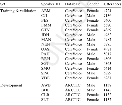
181 2.1. Speech data
182 Two speech databases are used in the evaluation of the
183 phonetic feature extraction, one for training and
cross-val-184 idation and the other for optimising the classifier
parame-185 ters. The speech data used here are summarised inTable 1.
186 For training and validation we use a large set of data
187 recorded as part of the development of the CereVoice speech
188 synthesis system. The database includes sub-corpora of
189 speech produced using lax, neutral and tense phonation
190 types in order to produce subtle changes in emotion (Aylett
191 and Pidcock, 2007). The acoustic characteristics of identical
192 phonemes produced in different phonation types can be
193 markedly different (e.g., with differences in spectral tilt,
pres-194 ence of noise in the spectrum etc). As we intend to use the 195 developed phonetic feature extraction on various types of 196 speech data (in future work), including expressive and
con-197 versational speech, incorporating this variety in the training
198
data is likely to increase the robustness of the feature
extrac-199
tion when applied to novel data. These sub-corpora have
200
been recorded over a five year period across several
lan-201
guages (English, French, German, Italian, Japanese),
how-202
ever we include only the English data here. The data
203
covers different accents of English (RP, General American,
204
Scottish accent, Irish accent, Northern England, Midlands).
205
For optimisation of classifier parameters, we use data
206
from 4 speakers (2 female, 2 male) from the ARCTIC
data-207
base (Kominek and Black, 2004). We label this as the
208
‘development’ set. Note that the use of a completely
sepa-209
rate database for parameter optimisation is done purposely
210
to avoid biasing results on the training and validation
211
database.
212
2.2. Classification
213
The approach used here is to develop classifiers of a set
214
of binary phonetic features. The phonetic features used
215
here are: {voiced, syllabic,1fricative, plosive, liquid, nasal}.
216
Although this set is not as exhaustive as that proposed in
217
Chomsky and Halle (1968), it does cover a reasonably large
218
set of phonetic features which are relevant to the speech
219
processing tasks considered in the present study. More
spe-220
cifically, for glottal source analysis it is clearly important to
221
detect voiced sounds. The turbulent air present in fricatives
222
and the potential zeros in the vocal tract spectrum for
223
nasals and liquids, may negatively affect the glottal inverse
224
filtering process. Similarly the rapid transitioning in
plo-225
sives is likely to cause difficulty for glottal analysis.
226
The classification task here is to map from a set of
227
acoustic features to binary labels, identifying the presence
228
or absence of a given phonetic feature.2
229
More formally, the classification problem involves
map-230
ping from the feature spaceI, inRn, to the target spaceT
231
(in this case {0, 1}, i.e. the individual phonetic feature
bin-232
ary target).
233
2.2.1. Acoustic features and target labelling
234
The standard Mel-frequency cepstral coefficients
235
[image:3.595.42.295.533.751.2](MFCCs) are used as the acoustic features in the present
Table 1
Summary of speech data used in training and validating of the phonetic feature extraction.
Set Speaker ID Database Gender Utterances Training & validation ABM CereVoice Female 4724
CJI CereVoice Male 7136 FES CereVoice Female 5400 FMM CereVoice Female 5580 GTV CereVoice Female 4869 JDH CereVoice Male 4982 MAN CereVoice Male 4982 NEN CereVoice Male 5785 OAS CereVoice Female 4981 PAH CereVoice Male 5017 RRH CereVoice Female 4806 SGT CereVoice Male 4363 SMO CereVoice Female 6414 SPA CereVoice Male 5829 VDE CereVoice Female 6281
Development AWB ARCTIC Male 1138
BDL ARCTIC Male 1142
CLB ARCTIC Female 1132 SLT ARCTIC Female 1132
1
We interpret the termsyllabicfollowingChomsky and Halle (1968)
whereby the feature is used to differentiate vowels from other classes of sounds. Note that consonants (such as liquids and nasals) that under certain circumstances may be½+syllabicare not labelled as syllabic in this study.
2
A note should be made here regarding the terminology. The classifi-cation problem addressed here, in fact, involves mapping from acoustic features to phonological labels. Indeed King and Taylor (2000) (and others) use the term phonological feature extraction which may appear more suitable. However, the use of binary phonological targets does not detract from the fact that phonetic variation within such phonological labels will inevitably affect the acoustic features and hence the classifica-tion output. Some authors have sought to circumvent this problem by using the termarticulatory feature extraction(Tarek and Carson-Bernd-sen, 2003), but this may conjure up connotations of physiological measurements. As a result we opt for the termphonetic feature extraction
236 study. The 13 MFCCs are measured on 25 ms Hanning
237 windowed frames with a 10 ms shift. The 0th cepstral
coef-238 ficient, corresponding to signal energy, is normalised to the 239 maximum value for a given utterance. First (D) and second 240 (D2) derivatives are also included, resulting in a 39-dimen-241 sional feature vector,x.
242 The binary target label for each phonetic feature is set
243 based on phonological labels derived following the forced
244 alignment (described below) of the speech data. For
exam-245 ple, for the phonetic feature ‘fricatives’, labels including /f/
246 and/z/ are assigned the target 1, with non-fricative labels
247 assigned the target 0.
248 Forced alignment was carried out using the CereProc
249 voice building system (Aylett and Pidcock, 2007). The
align-250 ment is a flat start monophone system which allows
pronun-251 ciation variation. The underlying system used to carry out
252 the alignment is HTK (Young et al., 2007) using a 10 ms
253 frame rate, a five state model, and based on MFCCs of 254 order 12 (plus log energy), and also first (D) and second 255 (D2) derivatives. The process is very similar to forced
align-256 ment described for Festival inRichmond et al. (2007),
how-257 ever, CereProc also employs proprietary techniques for
258 refining pause insertion and dealing with multiple
pronunci-259 ations. Tested against the CMU KED TIMIT database3
260 with just over 21 min of speech, the CereVoice aligner did
261 substantially better than the included festival based
align-262 ment (12% difference in insertion/deletion of segment
263 boundary compared to 21% in the CMU KED TIMIT
264 automatic labels, and a mean error of 10.1 ms for matching
265 segment boundaries compared to 11.2 ms error in the
Festi-266 val alignment). The speaker databases used in this study
267 contained over 10 times the material in this evaluation
cor-268 pus for each speaker and alignment results are likely to be 269 improved over this baseline evaluation.
270 2.2.2. Artificial Neural Networks – ANNs
271 The first classification approach included in the present
272 study is based on Artificial Neural Networks (ANNs).
273 ANNs are in general used for learning the mapping
func-274 tionffrom ItoT :fðxÞ:x2I!y2T, wherex denotes
275 the input vector andy the output of the approximatorf.
276 The ANN implementation we use here is based on the
277 multi-layer perceptron (MLP) as the network type of
278 choice which is said to fulfil the universal approximator 279 theorem (Hornik, 1991). We use a two layer MLP, with a
280 single hidden layer. The number of neurons used in the
hid-281 den layer is set below (Section 2.4). tanh is the transfer
282 function used by the hidden layer, while the output layer
283 uses a linear transfer function. Weight training is done
284 using the back-propagation algorithm (Bishop, 2006).
285 2.2.3. Gaussian Mixture Models – GMMs
286 The second classification approach utilises Gaussian
287 Mixture Models (GMMs). GMMs are a generative
288
learning algorithm which involve modelling a given class
289
of data using a mixture of multi-variate Gaussians. In
290
our current implementation we train a GMM for the data
291
where the given phonetic feature ispresentk1 and a sepa-292
rate GMM for where it isabsentk0.
293
A given GMM,k, has the probability density function:
294
pðxjkÞ ¼X
K
k¼1
Pk N ðxjlk;RkÞ ð1Þ
296 296
297
whereKis the number of multi-variate Gaussians,Pk is the
298
prior probability of the kth Gaussian and each Gaussian
299
can be written as:
300
N ðxjl;RkÞ ¼
1
ð2pÞm2jR
kj
2e 1
2ðxlkÞ
T
Rk1ðxlkÞ
ð2Þ 302302 303
wherex is the m dimensional feature vector (here m is 39,
304
see Section2.2.1),lkis its mean vector andRkis its m-by-m
305
covariance matrix. Here we use a diagonal covariance
306
matrix, and K is optimised on the development set as
307
described below (Section 2.4). The model parameters are
308
trained using the Expectation–Maximisation (EM)
309
algorithm (Bishop, 2006) with an initialisation step using
310
K-means clustering. A given phonetic feature is considered
311
to be present if:
312
pðxjk1Þ>pðxjk0Þ ð3Þ 314314
315
that is, if a given feature vector,x, is more likely to have
316
come from present phonetic feature GMM, k1, than the 317
absentone,k0.
318
2.2.4. Support Vector Machines – SVMs
319
The final classifier included in the present study is an
320
implementation of Support Vector Machines (SVMs).
321
SVMs in general look to find a separating hyperplane
322
which maximises the functional margin between the two
323
classes. In our SVM implementation we utilise a Radial
324
Basis Function (RBF) kernel (Bishop, 2006) which is used
325
to project the feature data into a higher-dimensional space
326
in order to derive a more effective separating hyperplane.
327
2.3. Experimental procedure
328
In order to validate the various classifiers used here for
329
the purpose of extracting phonetic features, we carry out
330
speaker independent leave-one-speaker-out validation
331
experiments. Here classifiers are trained on all but one
332
speaker’s data, and are then tested on the held out data.
333
The held out speaker is then rotated until all speakers have
334
been covered. The procedure is repeated for each of the six
335
phonetic features: {voiced, syllabic, fricative, plosive, liquid
336
and nasal}. We use three metrics to evaluate the
perfor-337
mance at the frame level. As percentage of errors (i.e.
per-338
centage of false positives and false negatives) is not a very
339
suitable metric for assessing classification for sparse
fea-340
341
F1¼ 2Tp
2TpþFpþFn2 ½0;1 ð4Þ
343 343
344 where Tp is the number of true positives, Fp is the number
345 of false positives ad Fn is the number of false negatives. We
346 also used False Positive Rate (FPR):
347
FPR¼ Fp
FpþTn100 ð5Þ
349 349
350 and True Positive Rate: 351
TPR¼ Tp
TpþFn100 ð6Þ
353 353
354 Note that during training the decision threshold, h, in
355 the ANN classifier is optimised by maximising F1 score
356 on the training set.
357 2.4. Classifier optimisation
358 In order to use our classifiers in our experiments we
359 must first optimise some of their parameters. These
param-360 eters are optimised on the development set summarised in 361 Table 1.
362 First we look to optimise the number of neurons used in 363 the hidden layer of the ANN classifier. This is done by
car-364 rying out a 10-fold cross validation procedure, where the
365 F1 score is recorded for each fold. In Fig. 1we illustrate
366 the effect of increasing the number of neurons used in the
367 hidden layer of the ANN by averaging across validation
368 folds and phonetic features (ALL – black line), and we also
369 show the effect separately for a selected sparse feature
370 (Nasal – red line) and for a well represented feature
371 (Syllabic – blue line). Overall there is no dramatic effect
372 of increasing the number of neurons on the feature
extrac-373 tion averaged across all phonetic features. Similarly, for the
374 syllabic feature, increasing the number of neurons does not
375 have a significant positive effect and there is even some
376
deterioration in F1 for higher numbers of neurons. For
377
the nasal feature, however, there is a clear improvement
378
with a higher number of neurons up to 64, after which
379
the effect plateaus. Based on this we opt to use 64 neurons
380
in our ANN implementation.
381
For the GMM classifier we carry out the same
proce-382
dure, but this time varying the number of Gaussians (i.e.
383
K) used in the GMM. The impact of this variation is
illus-384
trated inFig. 2. One can observe that the F1 score for the
385
syllabic feature plateaus from K set to 8. A similar effect is
386
observed the sparser nasal feature, and indeed for all
387
features combined, with no clear improvement observed
388
for K greater than 16. As a result, 16 Gaussians are used
389
our GMM implementation.
390
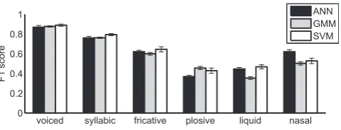
2.5. Results
391
Classification results for the phonetic features are shown
392
below for F1 (Fig. 3), FPR (Fig. 4) and and TPR (Fig. 5).
393
F1 score provides a good summary of detection
perfor-394
mance and will, hence, receive the most attention, although
395
FPR and TPR results will be referred to in order to help
396
explain the F1 score. Note that the results here are used
397
to determine which classifier should be used for each
2 4 8 16 32 64 128 256
0.4 0.5 0.6 0.7 0.8
Number of neurons
F1 score
[image:5.595.50.288.519.718.2]Syllabic Nasal ALL
Fig. 1. Effect of varying number of neurons used in the ANN classifier on F1 score. Data is expressed as meanstandard deviation.
2 4 8 16 32 64
0.2 0.3 0.4 0.5 0.6 0.7 0.8
Number of Gaussians
F1 score
[image:5.595.319.559.621.713.2]Syllabic Nasal ALL
Fig. 2. Effect of varying number of Gaussians used in the GMM classifier on F1 score. Data is expressed as meanstandard deviation.
voiced syllabic fricative plosive liquid nasal 0
0.2 0.4 0.6 0.8 1
F1 score
ANN GMM SVM
398 phonetic feature in the subsequent sections of this paper. If
399 there are no significant differences, we default to the ANN
400 classifier which is both computationally efficient at
run-401 time and which also can be used to output a contour which
402 can be interpreted as the posterior probability of the given
403 feature.
404 A two-way ANOVA with F1 score treated as the
depen-405 dent variable reveals a significant effect of both
indepen-406 dent variables: phonetic features [F(5,252)= 343.77, 407 p < 0.001] and classifier type [F(2,252)= 5.74, p < 0.01], as 408 well as the interaction of the two independent variables 409 [F(10,252)= 5.75, p < 0.001. Pair-wise comparisons using 410 Tukey’s Honestly Significant Difference (HSD) test shows
411 the SVM classifier produces significantly higher F1 scores
412 compared to the GMM classifier (p < 0.01). Although the
413 ANN classifier had a higher mean F1 score compared to
414 the GMM method, the difference was not found to be
sig-415 nificant (p = 0.07).
416 For the three phonetic features: voiced, syllabic and
fric-417 ative, no significant differences are observed between the
418 three classifiers, however SVM has a slightly higher mean
419 F1 owing to a relatively lower false positive rate. For
plo-420 sives, although the GMM classifier shows a higher false
421 positive rate, its higher true positive rate results in a signif-422 icantly higher F1 compared to the ANN classifier 423 (p < 0.05), though no significant difference compared to 424 the SVM. For liquid, the higher false positive rate for the
425 GMM method causes a significantly lower F1 compared
426 to both SVM and ANN classifiers (p < 0.05), though no
427 difference is observed between SVM and ANN. Finally,
428 for nasals the ANN classifier is found to have a
429 significantly higher F1 compared to both the GMM
430 (p < 0.001) and SVM (p < 0.05) methods.
431
Following the results observed in this section, we opt to
432
use the ANN classifier for all phonetic features except for
433
plosives, where the GMM classifier is instead used.
Consid-434
ering these particular phonetic feature extractors we briefly
435
assess here the false positives observed in the
speaker-inde-436
pendent experiments.Fig. 6summarises the distribution of
437
false positives for each of the phonetic feature extractors.
438
Note that this figure shows just the 5 most common false
439
positives. For voiced, /s/ and/t/ are the main false positives.
440
It is not uncommon that these phonologically voiceless
441
sounds would be subject to contextual voicing due to the
442
presence of adjacent voiced segments, e.g.,
inter-vocali-443
cally. For the remainder of the phonetic features, false
pos-444
itives are more evenly distributed across the different
445
sounds and in the majority of cases the substitution may
446
be somewhat explained by the co-articulatory influence of
447
surrounding segments. For fricative, for instance,
devoic-448
ing of /l/, /r/ and /E/, and aspirated or lenited realisation
449
of /t/ may partly explain the identification of these
seg-450
ments as fricatives.
451
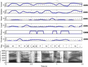
An example output of the entire phonetic feature
extrac-452
tion process is given inFig. 7. Besides the binary output of
453
the GMM feature extractor (used for plosives), one can
454
observe a continuous output for the ANN extractor.
Hav-455
ing continuous values for features like voiced and syllabic
456
provide additional information than simply the binary
457
decision, and may be useful for measuring aspects of the
458
speech signal like degree of voicing.4Focusing on the
out-459
put for nasals (third panel down) one can observe a clear
460
peak for the only nasal consonant present (/n/) at around
461
0.8 s. The liquid /r/ is detected (fourth panel down) at
462
around 0.45 and 1.25 s.
463
The output of the plosive GMM-based feature
extrac-464
tion (fifth panel down) reveals some interesting
informa-465
tion to do with the proposed approach. One can observe
466
that the /d/ (at around 0.6 s) and the /t/ (at around
467
1.15 s) are correctly identified. However, the first detected
468
plosive region at around 0.5 s (‘dh’ which corresponds to/
469
ð/) is counted as a false positive. In terms of the
phonolog-470
ical label it is in fact a false positive, but careful phonetic
471
analysis (using both auditory and spectrographic analysis)
472
shows that the degree of constriction is likely higher than
473
an idealised/ð/. This is of course a frequently occurring
474
process in continuous speech where the voiced fricative /
475
ð/ is realised as a plosive. The observation also seems to
476
further justify the terminology used of phonetic feature
477
extractionrather thanphonological feature extraction. This
478
may also somewhat explain the detected plosive at 0.95 s,
479
however the spectrogram shows acoustic characteristics
480
which look less like a plosive suggesting that this indeed
481
may be atruefalse positive.
482
Further, it is interesting to observe in the fricative
con-483
tour (sixth panel down), whereas the voiceless fricative voiced syllabic fricative plosive liquid nasal
0 10 20 30 40
FPR (%)
[image:6.595.38.281.69.158.2]ANN GMM SVM
Fig. 4. False positive rate (FPR)plotted as a function of phonetic class (ranked in ascending order of sparseness) for the three classifiers. Data is expressed as meanstandard error of the mean.
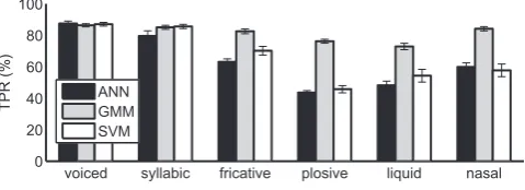
voiced syllabic fricative plosive liquid nasal 0
20 40 60 80 100
TPR (%)
ANN GMM SVM
Fig. 5. True positive rate (TPR)plotted as a function of phonetic class (ranked in ascending order of sparseness) for the three classifiers. Data is expressed as meanstandard error of the mean.
4 Note that although it is hypothesised that the ANN output may be an
[image:6.595.39.279.217.304.2]484 (‘th’ which corresponds to/h/) is clearly detected by the
485 feature extractor, the first ‘mistakenly’ detected plosive
486 /ð/ does not show a clear detection in the fricative contour.
487 This supports our claim here of higher degree of
constric-488 tion in the phonetic realisation of the sound, and also that
489 the feature extraction approach does indeed correspond
490 closely to the phonetics. For the /t/ at around 1.2 s, the
fric-491
ative contour slightly exceeds the decision threshold which
492
can be interpreted as a false positive. However, in the
spec-493
trogram one can observe the strong presence of noise and it
494
is likely that the feature extractor is detecting the aspiration
495
often accompanying voiceless stops as well as allophonic
496
lenition which entails these sounds being produced as
fric-497
atives. This once more highlights that potential for strong
s t k f p
0 10 20 30
False positive occurrence (%)
Voiced
s n t l r
0 10 20 30
Syllabic
s n l r z
0 10 20 30
Plosive
n t l r @
0 10 20 30
Transcription symbol
False positive occurrence (%)
Fricative
s t l r z
0 10 20 30
Transcription symbol Nasal
s n t z @
0 10 20 30
[image:7.595.159.449.69.308.2]Transcription symbol Liquid
Fig. 6. Summary of the false positives across all phonetic feature extractors. Note that the @ corresponds to/E/.
0 0.51
Voiced
0 0.51
Syllabic
0 0.5 1
Nasal
0 0.5 1
Liquid
0 0.51
Plosive
0 0.5 1
Fricative
0 0.5 1
pau ao th er ah v dh ax d ey n jh er t r ey l
Seg.
Time (s)
Frequency (Hz)
0 0.5 1 1.5
0 1000 2000 3000 4000 5000
ANN GMM ANN ANN ANN
ANN
Fig. 7. Output of the phonetic feature extraction, along with the segmentation and broadband spectrogram for the utterance“Author of The Danger Trail
[image:7.595.123.484.340.615.2]498 variation in the phonetic realisation of certain phonological
499 labels.
500 3. Context-sensitive glottal source processing
501 This section aims to utilise the information provided by
502 the automatic phonetic feature extraction to improve the
503 effectiveness of glottal source processing. The quantitative
504 assessment of glottal source analysis is known to be
prob-505 lematic. Some authors use methods including: analysis of 506 synthetic speech signals where parameter values are known 507 (Drugman et al., 2011; Kane and Gobl, 2013b), analysis of
508 natural speech with simultaneous Electroglottographic
509 recordings (from which reference parameters can be
510 derived, Kane and Gobl (2013a) and Sturmel et al.
511 (2006)) or analysis-synthesis procedures. All of these
meth-512 ods have their own serious shortcomings. In this study we
513 look to quantitatively evaluate the effectiveness of the
glot-514 tal source analysis implicitly through voice quality
classifi-515 cation experiments. The assumption here being that for
516 speech data involving voice quality variation brought
517 about by changes in laryngeal activity, effective glottal
518 source analysis will inevitably lead to successful
discrimina-519 tion of voice quality. Contrastingly, ineffective glottal 520 source parameterisation should result in a lack of discrim-521 ination of voice quality.
522 3.1. Speech data
523 In order to evaluate the glottal source analysis, we use a
524 subset of the speech data originally used inKane and Gobl
525 (2013c). In this database 17 TIMIT sentences were spoken 526 by 3 females and 3 males in a range of phonation types. In
527 the present study we use only those sentences spoken in
528 breathy, modal and tense phonation types. Additionally,
529 we include speech data from 3 male speakers, saying 10
530 sentences again in breathy, modal and tense phonation
531 types. This speech data was previously used in Kane and
532 Gobl (2013d), and details of the recording conditions and
533 setup are available in that publication.
534 3.2. Glottal source parameters
535 We use as feature data, both glottal source parameters
536 derived as direct measures from estimated glottal pulses
537 as well as parameters derived following the fitting of a
538 mathematical model to the pulses.5For both sets of
param-539 eters there are some prerequisites. First, glottal closure
540 instants (GCIs) are automatically detected from the speech
541 data using the SE-VQ algorithm (Kane and Gobl, 2013c),
542 which can be effective for analysis of non-modal phonation
543 types. We then use the iterative and adaptive inverse
filter-544 ing (IAIF) algorithm (Alku, 1992) in order to derive an
545
estimate of the glottal source signal. The IAIF algorithm
546
works by a sequence of all-pole modelling and inverse
fil-547
tering of vocal tract and glottal source components, with
548
increasing prediction order. Our IAIF implementation is
549
carried out pitch-synchronously, on GCI-centred analysis
550
frames with a duration of twice the local glottal period.
551
3.2.1. Direct measures
552
Four parameters measured directly from the estimated
553
glottal source signal are included in the present study.
554
Their inclusion is partly due to their effectiveness at
dis-555
criminating voice quality on a lax-tense dimension, as
dem-556
onstrated inAiras and Alku (2007). The first parameter is
557
the normalised amplitude quotient (NAQ, Alku et al.,
558
2002), which is derived using:
559
NAQ¼ fac
dpeakT0
ð7Þ
561 561
562
wherefacis the maximum amplitude of a given glottal flow
563
pulse,dpeak is the maximum negative amplitude of the
glot-564
tal derivative pulse (seeFig. 8) and andT0is the local glot-565
tal period. The quasi-open quotient (QOQ,Hacki, 1989) is
566
derived by normalising thequasi-open phase(see top panel
567
of Fig. 8)) to T0. The quasi-open phase is defined as the 568
duration between time points previous to and following
569
the maximum amplitude of the glottal flow pulse that
des-570
cend below 50% of this peak amplitude.
571
Two frequency domain parameters are also included.
572
The first is the difference in amplitude between the first
573
two harmonics of the narrowband glottal flow derivative
574
spectrum (H1–H2,Hanson, 1997). The spectrum is derived
575
using GCI-centred frames of duration three times the local
576
glottal period (to ensure clear harmonics) from the
esti-577
mated glottal flow derivative signal. Harmonic amplitudes
578
are measured by searching for peaks in the vicinity of
579
integer multiples of the localf0 in the spectrum. The final 580
parameter included is the so-called parabolic spectral
0 0.005 0.01 0.015 0.02
0 0.1 0.2 0.3 0.4
Time (s)
Amplitude
Glottal flow
f ac
0 0.005 0.01 0.015 0.02
−0.03 −0.02 −0.01 0 0.01
Time (s)
Amplitude
Glottal flow derivative
dpeak Quasi−open phase
[image:8.595.308.548.529.709.2]T0
Fig. 8. Glottal flow (top panel) and glottal flow derivative (bottom panel) pulses estimated by IAIF. Highlighted are the measurements required for calculating NAQ (i.e.facanddpeak) and QOQ (i.e. the quasi-open phase).
5 Note that many of the algorithms used here are freely available on the
581 parameter (PSP, Alku et al., 1997). The parameter is
582 derived by fitting a parabola to the low-frequency part of
583 the spectrum of a single glottal flow pulse.
584 3.2.2. Model-based measures
585 We also include glottal source parameters derived from
586 the Liljencrants–Fant (LF) glottal source model (Fant
587 et al., 1985a) fitted to estimated glottal flow derivative
588 pulses. We use the recently proposed dyProg-LF algorithm
589 (Kane and Gobl, 2013a). The method utilises a dynamic
590 programming algorithm, the weights for which are
opti-591 mised using manually-obtained glottal source analysis.
592 The target cost consists of a weighted time-domain and
fre-593 quency domain error measurement to ensure
comprehen-594 sive modelling of glottal pulses. A transition cost is 595 incorporated to ensure sensibly smooth parameter trajecto-596 ries. The transition cost is modulated by a
spectral-stationa-597 rity measure to allow rapidly varying parameter values in
598 certain speech regions (e.g., voice-offset, creaky or harsh
599 voice). Three parameters derived from the LF model fit
600 are used as part of the present feature data: Rg (normalised
601 frequency of the glottal formant), Rk (a measure of glottal
602 skew, and inverse of the commonly used speed quotient)
603 and Ra (a measure of the glottal return phase).
604 3.3. Experimental procedure
605 The 7 glottal parameters (i.e. {NAQ, QOQ, H1-H2,
606 PSP, Rg, Rk, Ra}) are extracted from the speech data at
607 locations corresponding to GCIs. Only GCIs in voiced
608 regions (as determined using the phonetic feature
extrac-609 tion method) are used. Along with the glottal parameters,
610 we also extract and record the output of the optimal
pho-611 netic feature extractors at these locations. This makes up
612 our feature data to be used.
613 For the classification, we utilise an SVM
implementa-614 tion with a one-against-one multi-class architecture. As
615 with the phonetic feature extraction, we use a RBF kernel.
616 The targets used in the classification experiments are the
617 three voice quality labels: {breathy, modal, tense}. 10-fold
618 cross-validation experiments are carried out where the data
619 is randomly separated into 10 equal sized sets. Training is 620 carried out on 9 of the sets with testing on the one held
621 out set. The procedure is repeated by varying the held
622
out set until all 10 sets have been covered. Classification
623
error and confusion matrices are recorded.
624
In order to examine the effect of including only selected
625
glottal feature data we repeat the cross-validation
experi-626
ments for 6 different feature sets:
627
All: Including glottal feature data from all voiced
628
regions (used as a baseline).
629
No-liquid: Baseline feature set, excluding data from
630
detected liquid regions.
631
No-nasal: Baseline feature set, excluding data from
632
detected nasal regions.
633
No-fricative: Baseline feature set, excluding data from
634
detected fricative regions.
635
No-plosive: Baseline feature set, excluding data from
636
detected plosive regions.
637
Only-syllabic: Only feature data from detected syllabic
638
regions
639
640
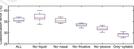
3.4. Results
641
The results from the voice quality classification
experi-642
ments are illustrated in Fig. 9, where classification error
643
(%) from the 10-fold cross-validation is plotted as a
func-644
tion of feature set used. It is clear fromFig. 9that choosing
645
to include or exclude glottal source feature data from
cer-646
tain phonetic regions has a significant effect on the
classifi-647
cation error. This observation is supported by results from
648
a one-way ANOVA where feature set (i.e. the independent
649
variable) is found to have a highly significant effect
650
[F(5,54)= 64.0, p < 0.0001] on the classification error (i.e. 651
dependent variable).
652
A further statistical analysis using Tukey’s Honestly
Sig-653
nificant Difference (HSD) test allows pairwise comparisons
654
of the various feature sets. Excluding liquid regions
actu-655
ally increases the median classification error (to 38.5%)
656
but with no significant difference compared to the baseline
657
(i.e. feature data from all regions, which gives a median
658
classification error of 35.6%). This suggests that glottal
fea-659
ture data derived in liquid regions is in fact beneficial,
660
rather then harmful, to voice quality classification.
661
Excluding nasal regions brings a slight reduction in the
662
median classification error (34.2%), but again with no
sig-ALL No−liquid No−nasal No−fricative No−plosive Only−syllabic 25
30 35 40
[image:9.595.162.443.607.711.2]Classification error (%)
663 nificant difference compared to the baseline. This finding
664 does not strictly corroborate the initial findings reported
665 in Kane et al. (2013b), where we found a significant 666 improvement in classification when excluding nasal 667 regions. However, despite the improvement being
signifi-668 cant the amplitude of the difference was relatively small.
669 Another important difference is that our detection of nasal
670 regions is significantly more accurate in the present study
671 compared to that in Kane et al. (2013b). It may be that
672 the false positives resulting from the previous nasal
detec-673 tion method were in fact also useful to exclude from the
674 features used in the classifier.
675 Excluding feature data from fricative regions brings a
676 highly significant (p < 0.0001) reduction in classification
677 error (median error of 33.6%), corroborating our previous
678 findings (Kane et al., 2013b). Excluding plosive regions
679 results in an even larger reduction in classification error 680 (median error of 32.1 %) relative to the baseline 681 (p < 0.0001) and also compared with results from removing 682 fricative regions (p = 0.05). The largest reduction in
classi-683 fication error is achieved by only utilising glottal feature
684 data obtained in detected syllabic regions (28.2% median
685 error), with a 7.4% reduction in median classification error
686 compared to using feature data from all speech regions.
687 The reduction is further reported from the pairwise
com-688 parisons which reveal a highly significant difference
689 (p < 0.0001) compared to every other feature set.
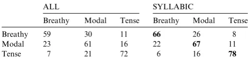
690 Finally, confusion matrices for the ‘all’ feature set and
691 the ‘syllabic’ feature set are shown inTable 2. The matrices
692 demonstrate an even classification improvement across the
693 three voice quality labels. This suggests that the approach
694 of isolating syllabic regions is helpful generally for 695 improving the classification of voice quality and not solely 696 for one voice quality class.
697 4. Discussion & conclusion
698 This study looked to implement and evaluate a variety 699 of approaches for automatically determining information 700 on the presence of an array of binary phonetic features.
701 We then looked to apply this information to allow glottal
702 source processing which is sensitive to the underlying
pho-703 netic context. In particular, we implicitly evaluated the
704 effectiveness of glottal source analysis through a set of
705 voice quality classification experiments.
706 In response to the first research question (RQ 1, at the
707 end of Section1) we implemented and evaluated classifiers
708
based on ANNs, GMMs and SVMs on a vast speech
data-709
set covering a range of speakers. The data consisted of
710
speech produced in a variety of phonation types which is
711
likely to enhance the robustness of the feature extraction
712
when applied to expressive speech. In terms of hypothesis
713
1.1, we indeed do generally observe a decrease in accuracy
714
with increasing sparseness of the given feature. However,
715
sparseness in not the only issue affecting accuracy, as
dem-716
onstrated by the higher accuracy for nasals compared to
717
the less sparse plosives and liquids. This is likely due to
718
the more stable spectral characteristics of nasals compared
719
to plosives, which often display a relatively long period
720
with very low signal energy.
721
We in general observe higher accuracy for the
discrimi-722
native classifiers (i.e. ANNs and SVMs) compared to the
723
generative classifier, GMM. This is with the exception of
724
plosives, where the GMM-based classifier gives the best
725
accuracy. It is rather difficult to speculate on why the
726
GMM classifier is most effective for plosives. One
explana-727
tion, however, could be that plosives, unlike the other
clas-728
ses of speech sounds included here, are highly varied,
729
dynamic events with combinations of a hold phase and
730
release burst. Using multiple Gaussians in a GMM may
731
be useful for modelling these separate acoustic
characteris-732
tics which both come under the single class ’plosive’ and,
733
hence, this approach may be most effective for modelling
734
this specific speech feature.
735
For SVMs, which we initially hypothesised (hypothesis
736
1.2 to be effective with handling sparse features, we in
737
general observe a similar level of performance to the
738
ANN classifier (with nasals being an exception). Note that
739
SVMs are not found, for any phonetic feature, to
signifi-740
cantly outperform the ANNs. Although the SVMs provide
741
significantly better detection of liquids than the GMMs, for
742
the other sparse features the SVMs provide a similar or
743
worse level of detection compared to the GMMs.
There-744
fore, we cannot confirm hypothesis 1.2 and conclude that
745
SVMs are particularly suited to the classification of sparse
746
phonetic features.
747
We address RQ 2 by investigating the extent to which
748
this information can be useful for improving the
effective-749
ness of glottal source analysis. Evidence from the voice
750
quality classification experiments strongly suggests that
751
indeed the effectiveness of glottal source analysis can be
sig-752
nificantly improved. In relation to hypothesis 2.1, nasals
753
only appear to be slightly problematic for glottal analysis,
754
as suggested by the minor reduction in classification by
755
excluding feature data derived in nasal regions. This
find-756
ing is somewhat at odds to the findings inGobl and
Mahs-757
hie (2013), however in that paper the authors found that
758
nasalisation had the main negative impact on glottal return
759
phase parameter estimation. As the voice quality
classifica-760
tion experiments used in this study exploited a variety of
761
parameters to do with both the glottal open and return
762
phases the overall accuracy was not negatively affected
763
for nasals. One must also bear in mind that voice quality
764
[image:10.595.31.284.110.171.2]classification can only provide a rather crude assessment
Table 2
Confusion matrices for the voice quality classification experiment, shown for the classifier trained with all data (left column) and with only data in syllabic regions (right column).
Q5
ALL SYLLABIC
Breathy Modal Tense Breathy Modal Tense
Breathy 59 30 11 66 26 8
Modal 23 61 16 22 67 11
765 of glottal source analysis. Nevertheless, this approach is
766 necessary for quantitative evaluation on a large body of
767 data.
768 Removal of feature data from fricative regions, how-769 ever, brings a significant improvement in classification 770 error. The best classification accuracy is achieved by only
771 using glottal feature data derived in detected syllabic
772 regions. This finding supports the previous strategy applied
773 by Mokhtari and Campbell (2003) for targeting specific
774 speech regions for voice quality analysis. Recall, however,
775 that those authors did not explicitly examine the
improve-776 ment in voice quality classification using their selection
777 approach compared to using all voiced speech regions.
778 Our findings quantitatively demonstrate that syllabic
779 regions are indeed the most reliable phonetic region for
780 effective glottal source analysis and that the proposed
pho-781 netic feature extraction is a suitable and robust means for
782 determining this information automatically. Also, as is dis-783 cussed in the introduction, syllabic regions may be the 784 parts of speech where we most portray our vocal timbre,
785 so we must consider that this too may have affected the
786 classification results favourably.
787 We intend to apply the proposed phonetic feature
788 extraction approach, in particular the determination of
syl-789 labic regions, to our analysis of expressive and
conversa-790 tional speech. Furthermore, we wish to investigate
791 whether the information provided by the phonetic feature
792 extraction can be used to enable an adaptive vocal tract
793 model to improve glottal inverse filtering, and indeed the
794 parameterisation of speech in general. Finally, the
795 approach of phonetic feature extraction may be exploited
796 in clinical settings to help allow clinicians analyse read
797 and spontaneous speech and alleviate some of the problems 798 of analysing sustained vowels (e.g., the unnatural ‘singing’ 799 production which has little in common with the habitual
800 voice of a speaker).
801 Acknowledgements
802 The first, third and fourth authors are supported by the
803 Science Foundation Ireland Grant 09/IN.1/I2631
804 (FASTNET).
805 References
806 Airas, M., Alku, P., 2007. Comparison of multiple voice source param-807 eters in different phonation types. In: Proceedings of Interspeech 2007, 808 Antwerp, Belgium, pp. 1410–1413.
809 Ali, A.M.A., der Spiegel, J.V., Mueller, P., Haentjens, G., Berman, J., 810 1999. An acoustic-phonetic feature-based system for automatic pho-811 neme recognition in continuous speech. In: Proceedings of the IEEE 812 International Symposium on Circuits and Systems 3, pp. 118–121. 813 Alku, P., 1992. Glottal wave analysis with pitch synchronous iterative 814 adaptive inverse filtering. Speech Commun. 11 (2-3), 109–118. 815 Alku, P., 2011. Glottal inverse filtering analysis of human voice produc-816 tion – a review of estimation and parameterization methods of the 817 glottal excitation and their applications. Sadhana 36 (5), 623–650. 818 Alku, P., Vilkman, E., 1994. Estimation of the glottal pulseform based 819 on discrete all-pole modeling. In: Proceedings of the Third
Inter-820 national Conference on Spoken Language Processing, pp. 1619–
821 1622.
822 Alku, P., Strik, H., Vilkman, E., 1997. Parabolic spectral parameter – a
823 new method for quantification of the glottal flow. Speech Commun. 22
824 (1), 67–79.
825 Alku, P., Ba¨ckstro¨m, T., Vilkman, E., 2002. Normalized amplitude
826 quotient for parameterization of the glottal flow. J. Acoust. Soc. Am.
827 112 (2), 701–710.
828 Alku, P., Pohjalainen, J., Vainio, M., Laukkanen, A., Story, B., 2013.
829 Formant frequency estimation of high-pitched vowels using weighted
830 linear prediction. J. Acoust. Soc. Am. 134 (2), 1295–1313.
831 Aylett, M.P., Pidcock, C.J., 2007. The CereVoice characterful speech
832 synthesiser SDK. In: Artificial Intelligence and Simulation of
Behav-833 iour (AISB). Newcastle, UK.
834 Bishop, C.M., 2006. Pattern Recognition and Machine Learning
(Infor-835 mation Science and Statistics). Springer-Verlag, New York.
836 Campbell, N., Mokhtari, P., 2003. Voice quality: the 4th prosodic
837 dimension. In: Proceedings of the 15th International Congress of
838 Phonetic Sciences, pp. 2417–2420.
839 Chan, W., Zheng, N., Lee, T., 2007. Discrimination power of vocal source
840 and vocal tract related features for speaker segmentation. IEEE Trans.
841 Audio Speech Lang. process. 15 (6), 1884–1892.
842 Chomsky, N., Halle, M., 1968. The Sound Pattern of English. MIT Press,
843 Cambridge, MA.
844 Cullen, A., Kane, J., Drugman, T., Harte, N., 2013. Creaky voice and the
845 classification of affect. In: Proceedings of WASSS, Grenoble, France.
846 Drugman, T., Bozkurt, B., Dutoit, T., 2011. A comparative study of
847 glottal source estimation techniques. Comput. Speech Lang. 26, 20–34.
848 Fant, G., 1960. The Acoustic Theory of Speech Production, 2nd ed.
849 Mouton, Hague, 1970.
850 Fant, G., Lin, Q., 1987. Glottal source – vocal tract acoustic interaction.
851 KTH, Speech Transmission Laboratory, Quarterly Report 28 (1), pp.
852 13–27.
853 Fant, G., Liljencrants, J., Lin, Q., 1985. A four parameter model of glottal
854 flow. KTH, Speech Transmission Laboratory, Quarterly Report 4, pp.
855 1–13.
856 Fant, G., Lin, Q., Gobl, C., 1985b. Notes on glottal flow interaction.
857 KTH, Speech Transmission Laboratory, Quarterly Report 2-3, 21–45.
858 Gobl, C., Mahshie, J., 2013. Inverse filtering of nasalized vowels using
859 synthesized speech. J.Voice 27 (2), 155–169.
860 Hacki, T., 1989. Klassifizierung von glottisdysfunktionen mit hilfe der
861 elektroglottographie. Folia Phoniatrica, 43–48.
862 Hanson, H.M., 1997. Glottal characteristics of female speakers: acoustic
863 correlates. J. Acoust. Soc. Am. 10 (1), 466–481.
864 Hornik, K., 1991. Approximation capabilities of multilayer feedforward
865 networks. Neural Networks 4 (2), 251–257.
866 Iliev, I., Scordilis, M., Papa, J., Falco, A., 2010. Spoken emotion
867 recognition through optimum-path forest classification using glottal
868 features. Comput. Speech Lang. 24 (3), 445–460.
869 Kane, J., Gobl, C., 2013a. Automating manual user strategies for precise
870 voice source analysis. Speech Commun. 55 (3), 397–414.
871 Kane, J., Gobl, C., 2013. Evaluation of automatic glottal source analysis.
872 In: Proceedings of NOLISP, Mons, Belgium, pp. 1–8.
873 Kane, J., Gobl, C., 2013c. Evaluation of glottal closure instant detection
874 in a range of voice qualities. Speech Commun. 55 (2), 295–314.
875 Kane, J., Gobl, C., 2013d. Wavelet maxima dispersion for breathy to tense
876 voice discrimination. IEEE Trans. Audio Speech Lang. Process. 21 (6),
877 1170–1179.
878 Kane, J., Scherer, S., Aylett, M., Morency, L., Gobl, C., 2013. Speaker
879 and language independent voice quality classification applied to
880 unlabelled corpora of expressive speech. In: Proceedings of ICASSP,
881 Vancouver, Canada.
882 Kane, J., Yanushevskaya, I., Dalton, J., Gobl, C., Nı´Chasaide, A., 2013.
883 Using phonetic feature extraction to determine optimal speech regions
884 for maximising the effectiveness of glottal source analysis. In:
885 Proceedings of Interspeech, Lyon, France.
886 Kanokphara, S., Macek, J., Carson-berndsen, J., 2006. Comparative
888 In: Proceedings of the 19th International Conference on Industrial, 889 Engineering and Other Applications of Applied Intelligent Systems. 890 King, S., Taylor, P., 2000. Detection of phonological features in 891 continuous speech using neural networks. Comput. Speech Lang. 14, 892 333–353.
893 Kominek, J., Black, A., 2004. The CMU ARCTIC speech synthesis 894 databases. ISCA speech synthesis workshop, Pittsburgh, PA, pp. 223– 895 224.<http://festvox.org/cmuarctic/>
896 Launay, B., Siohan, O., Surendran, A., Lee, C., 2002. Towards knowl-897 edge-based features for hmm based large vocabulary automatic speech 898 recognition. In: Proceedings of ICASSP, Orlando, Florida, USA, pp. 899 817–820.
900 Lin, Q., 1987. Nonlinear interaction in voice production. KTH, Speech 901 Transmission Laboratory, Quarterly Report 28 (1), pp. 1–12. 902 Lugger, M., Yang, B., 2008. Cascaded emotion classification via psycho-903 logical emotion dimensions using a large set of voice quality 904 parameters. In: Proceedings of ICASSP, Las Vegas, Nevada, USA, 905 pp. 4945–4948.
906 Mokhtari, P., Campbell, N., 2002. Automatic detection of acoustic centres 907 of reliability for tagging paralinguistic information in expressive speech. 908 In: Proceedings of Language Resources and Evaluation (LREC). 909 Mokhtari, P., Campbell, N., 2003. Automatic measurement of pressed/ 910 breathy phonation at acoustic centres of reliability in continuous 911 speech. IEICE Transactions on Information and Systems (special issue 912 on speech information processing) E-86-D(3), pp. 574–582.
913 Murty, K., Yegnanarayana, B., 2006. Combining evidence from residual 914 phase and mfcc features for speaker recognition. IEEE Signal 915 Processing Lett. 13 (1), 52–55.
916 Raitio, T., Suni, A., Yamagishi, J., Pulakka, H., Nurminen, J., Vainio, 917 M., Alku, P., 2011. HMM-based speech synthesis utilizing glottal 918 inverse filtering. IEEE Trans. Audio Speech Lang. process. 19 (1), 919 153–165 (1).
920 Raitio, T., Suni, A., Vainio, M., Alku, P., 2013. Synthesis and perception 921 of breathy, normal, and lombard speech in the presence of noise. 922Q4 Computer Speech and Language (in press).
923 Richmond, K., Strom, V., Clark, R., Yamagishi, J., Fitt, S., 2007. Festival
924 multisyn voices for the 2007 blizzard challenge. In: Proc. Blizzard
925 Challenge Workshop (in Proc. SSW6), Bonn, Germany.
926 Siniscalchi, S., Lee, C., 2009. A study on integrating acoustic-phonetic
927 information into lattice rescoring for automatic speech recognition.
928 Speech Commun. 51 (11), 1139–1153.
929 Siniscalchi, S., Yu, D., Deng, L., Lee, C., 2013. Exploiting deep neural
930 networks for detection-based speech recognition. Neurocomputing
931 106, 148–157.
932 Sturmel, N., d’Alessandro, C., Doval, B., 2006. A spectral method for
933 estimation of the voice speed quotient and evaluation using
electro-934 glottography. In: 7th Conference on Advances in Quantitative
935 Laryngology, Groningen, The Netherlands.
936 Sze´kely, E´ ., Kane, J., Scherer, S., Gobl, C., Carson-Berndsen, J., 2012.
937 Detecting a targeted voice style in an audiobook using voice quality
938 features. In: Proceedings of ICASSP, Kyoto, Japan, 4593–4596.
939 Tarek, A., Carson-Berndsen, J., 2003. HARTFEX: a multi-dimentional
940 system of HMM based recognisers for articulatory features extraction.
941 In: Proceedings of Non-Linear Speech Processing Workshop
942 (NOLISP03).
943 Teager, H.M., Teager, S.M., 1990. Evidence for nonlinear sound
944 production mechanisms in the vocal tract. In: Hardcastle, W.J.,
945 Marchal, A. (Eds.), Speech Production and Speech Modelling. Kluwer
946 Academic, pp. 241–261.
947 Walker, J., Murphy, P., 2007. A review of glottal waveform analysis. In:
948 Stylianou, Y., Faundez-Zanuy, M., Esposito, A. (Eds.), Progress in
949 Nonlinear Speech Processing. Springer Verlag, pp. 1–21.
950 Young, Steve J., Kershaw, D., Odell, J., Ollason, D., Valtchev, V.,
951 Woodland, P., 2007. The HTK Book Version 3.4. Cambridge
952 University Press.
953 Yu, D., Siniscalchi, S., Deng, L., Lee, C., 2012. Boosting attribute and
954 phone estimation accuracies with deep neural networks for
detection-955 based speech recognition. In: Proceedings of ICASSP, pp. 4169–4172.
956 Zheng, N., Lee, T., Ching, P., 2007. Integration of complementary
957 acoustic features for speaker recognition. IEEE Signal Processing Lett.
958 14 (3), 181–184.