warwick.ac.uk/lib-publications
Llano, Danilo X and McMahon, Richard A.. (2017) Control techniques with system efficiency
comparison for micro-wind turbines. IEEE Transactions on Sustainable Energy, 8 (4). pp.
1609-1617.
Permanent WRAP URL:
http://wrap.warwick.ac.uk/96928
Copyright and reuse:
The Warwick Research Archive Portal (WRAP) makes this work by researchers of the
University of Warwick available open access under the following conditions. Copyright ©
and all moral rights to the version of the paper presented here belong to the individual
author(s) and/or other copyright owners. To the extent reasonable and practicable the
material made available in WRAP has been checked for eligibility before being made
available.
Copies of full items can be used for personal research or study, educational, or not-for profit
purposes without prior permission or charge. Provided that the authors, title and full
bibliographic details are credited, a hyperlink and/or URL is given for the original metadata
page and the content is not changed in any way.
Publisher’s statement:
“© 2017 IEEE. Personal use of this material is permitted. Permission from IEEE must be
obtained for all other uses, in any current or future media, including reprinting
/republishing this material for advertising or promotional purposes, creating new collective
works, for resale or redistribution to servers or lists, or reuse of any copyrighted component
of this work in other works.”
A note on versions:
The version presented here may differ from the published version or, version of record, if
you wish to cite this item you are advised to consult the publisher’s version. Please see the
‘permanent WRAP URL’ above for details on accessing the published version and note that
access may require a subscription.
1
Control techniques with system efficiency
comparison for micro-wind turbines
Danilo X Llano and Richard A McMahon
Abstract—This paper presents the implementation of a
sensor-less speed controller and active rectification in a micro-wind turbine intended for battery charging. The controller was tested in a wind turbine emulator test rig using real wind data available from British bases in Antarctica. The control algorithm was successfully tested up to 14 m/s wind speed. Beyond this point the electrical unbalance in the turbine generator compromised the stability and performance of the system.
Also, a system efficiency comparison of different control algorithms is given to demonstrate the advantages of using active rectification instead of passive diode rectifiers in micro-wind turbines. This comparison was done between the sensorless control plus active rectifier, a DC-DC converter regulator and the direct connection between the turbine and battery by means of a diode rectifier. The turbine with an active rectifier and sensorless control achieved the highest power coefficient over the range of wind speeds showing that this technique is an attractive and relatively low cost solution for maintaining good performance of micro-wind turbines at low and moderate wind speeds.
Index Terms—Micro wind turbine, wind emulator test-rig,
active rectification, sensorless speed control.
I. INTRODUCTION
M
ICRO-wind turbines intended for battery charging have been used for decades. Indeed, they were the most commonly available devices (in limited numbers) in the wind energy market before the first oil price shock in early 1970s. After that crisis there was increasing interest and financial support in different countries such as Germany, Denmark, Sweden and the US to develop reliable and efficient large wind turbines (MW range) for power generation. The main aim at that time was looking at the diversification of power sources and reducing the dependency on fossil fuels coming from third party countries [1]. Micro-wind turbines have also been developed since then, with better aerodynamical design, more efficient electrical generators, improved materials and manufacturing processes. However, the power conversion stage has not changed significantly; passive rectification and DC to DC converters are the industry standard in micro-wind turbines [2].This research was supported by the Semiconductor Research Corporation (SRC) and the Texas Analog Center of Excellence (TxACE) through the Task ID: 1836.069, Electronic Systems for Small Wind Turbines and NERC IAA Knowledge Exchange Awards in collaboration with the British Antarctic Survey (BAS)
Danilo X Llano was with the Electrical Engineering Division, University of Cambridge, 9 JJ Thompson CB3 0FA, Cambridge - UK. He is now with the Warwick Manufacturing Group, University of Warwick, Coventry CV4 7AL (email:[email protected] / [email protected])
Richard A McMahon was with the Electrical Engineering Division, Uni-versity of Cambridge, 9 JJ Thompson CB3 0FA, Cambridge - UK. He is now with the Warwick Manufacturing Group, University of Warwick, Coventry CV4 7AL ([email protected])
Some micro-wind turbines can be directly connected to a lead acid battery but this is not recommended by most of the manufacturers because the system does not have any control over charging. The battery can experience excessive charge rates and overcharging, which might lead to permanent dam-age. Manufacturers usually sell the turbine with a controller. The standard topology is a boost/buck converter to manage the battery charging cycle and a dump resistor to dissipate excess energy as heat if required (when the battery is fully charged). Otherwise, if the turbine is unloaded and the wind is blowing, the turbine will accelerate uncontrollably to high rotational speeds that could lead to damage [3]–[5].
Active rectification has not been explored at this power level (up to 250 W), presumably due to the extra costs associated with an active rectifier, its controller and sensors, and higher complexity in electronics and control algorithms. In addition, some micro-wind turbines have a built-in diode rectifier and then the DC power is transmitted via slip rings and brushes mounted on the turbine post. This mechanical arrangement enables passive yaw control by a tail blade that allows the turbine to align itself with the wind direction for better performance, but limits any chance of installing an active rectifier without providing an additional slip ring.
Aside from mechanical constraints, sensorless speed control and active rectification are an attractive option for micro-wind turbines from the economic and energy production points of view. The significant cost of the speed sensor (usually an optical encoder) is completely eliminated. The price of voltage and current sensors is also reduced since low-cost voltage dividers and shunt resistors can be straightforwardly used as sensors at this power range. In addition, relatively high performance microcontrollers (for running digital control algorithms), medium power MOSFETs and their drivers (for the active rectifier) are available in the market at competitive prices. Micro-wind turbines can achieve relatively high shaft speeds (up to 1500 RPM) at a terminal voltage suitable for connection to a 12 or 24 V battery [4], [5], so that MOSFETs are suitable switching devices.
Sensorless speed control is indeed technically challenging and not completely understood and developed for this par-ticular application. In terms of control and speed estimation algorithms, a robust and reliable technique is required to compensate for the uncertainty in parameters, issues due to the machine construction, and varying and potentially harsh work-ing conditions. Also, micro-wind turbines have fast dynamics since their mechanical inertia is much lower in comparison to medium or big wind turbines.
curves when the turbine is directly wired to a lead acid battery are provided as they are not given by manufacturers, but they are instrumental especially for understanding the dynamics of the system running without any electronic control (just the diode rectifier). These charging curves are also used in the efficiency comparison section. Later on, this paper describes the implementation of a sensorless speed controller for a micro-wind turbine with verification in an emulator test rig. Additionally, controller and system stability issues due to the unbalances in the generator are studied from an analytical and experimental approach to provide limiting working conditions. Finally, a system efficiency comparison of different control techniques was performed to show the advantages of active rectification in terms of overall power generation.
Common symbols used throughout the paper are presented in Table I.
Symbol Description
Ldq dq inductance
Rs Phase resistance
ωm Rotor speed
J Turbine Inertia
P Pole-pairs
φ Rotor flux
Ts Sampling time
idq dq stator currents
udq dq stator voltages
Cp Power coefficient
λ Tip speed ratio
Tem Electromagnetic torque
[image:3.595.313.554.67.141.2]TL Load torque (wind torque)
Table I: Common Symbols
II. RUTLAND913WIND TURBINE
The wind turbine chosen for this study was a Rutland 913 model. This micro-wind turbine is widely available in the market and specifically designed for battery charging. It is a six bladed, horizontal axis, turbine based on a direct drive PM generator, without active pitch or yaw control. The generator is a three phase, star connected, axial flux, permanent magnet machine. Equations (1) and (2) describe the PM generator in thedq reference frame [6]
ud = Rsid+Ld
did
dt −LqiqP ωm (1)
uq = Rsiq+Lq
diq
dt +LdidP ωm+P ωmφ (2)
The terms−LqiqP ωmin (1) andLdidP ωm+P ωmφin (2) are coupling terms.
An approximate model for the power coefficient,CP, of the Rutland turbine is given by (3)
λi λ
It is assumed that the turbine blades are aligned with the wind direction due to the passive yaw control (tail blade).
Table II summarises the most important parameters of the turbine and its generator. The electrical parameters were estimated from tests and the performance parameters were estimated from wind tunnel measurements as described in subsection IV-A. The convention in [7], [8] was used, where the d-axis is aligned with the magnets, thereforeLq > Ld.
Parameter value
Phase resistance(Rs) 0.8Ω
Direct inductance(Ld) 0.87 mH Quadrature inductance(Lq) 1.31 mH
Voltage constant(kv) 45.2 mVp/RPM (mean value)
Pole pairs(P) 4
Maximum power coefficient(Cpmax) 0.25 (mean value) Optimal tip speed ratio(λopt) 3.75 (mean value)
Blade radius(r) 0.455 m
Rated power (maximum) 250 W
Table II: Wind turbine specifications
III. EMULATOR TEST-RIG
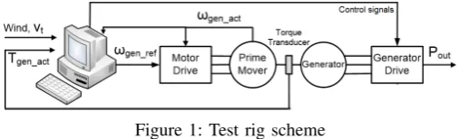
[image:3.595.302.556.245.345.2]A micro-wind turbine emulator test rig has been built up to replicate the behaviour of a real wind turbine [9], [10]. The prime mover is a servomotor rated at 3000 RPM, 19 Nm and 4.5 kW. It is controlled with an industrial drive and a target machine manufactured by Speedgoat that executes in real time the micro-wind turbine model described by (3) which is implemented in MATLAB/Simulink. A torque & speed transducer and an encoder are also included. Fig. 1 and 2 show the test rig diagrammatically and its physical realisation respectively.
Figure 1: Test rig scheme
IV. TURBINECHARACTERISATION ANDCONTROL
[image:3.595.302.556.521.598.2]Figure 2: Test rig set up
A. Wind tunnel measurements
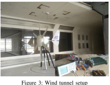
[image:4.595.312.533.62.175.2]The Rutland 913 wind turbine was installed in a wind tunnel to measure the power coefficient versus tip speed ratio curves at various wind speeds. Fig. 3 shows the setup. The experiment was carried out as follows: the wind turbine was aligned with the wind direction. The turbine has a built-in diode rectifier that was loaded by a variable resistance. The wind speed was set by the tunnel and the operating point was changed with the variable load resistance. The shaft speed was found from the frequency of the line voltage measured with a differential probe and oscilloscope. Power and shaft speed were recorded at various operational points for different wind speeds. The correction factors proposed in [11], [12] were applied to take into account the tunnel blockage due to the tunnel walls.
[image:4.595.71.263.401.548.2]Figure 3: Wind tunnel setup
Fig. 4 shows the power coefficient versus tip speed ratio curves of the Rutland turbine at different wind speeds meas-ured in the wind tunnel. The measurement points at different wind speeds present a noticeable trend which matches the model described in (3).
B. Turbine directly wired to a lead acid battery
The Rutland 913 turbine has a built-in three phase diode rectifier that was directly wired to two lead acid batteries connected in parallel to match the battery specification given by the turbine manufacturer. The batteries are Yuasa series NP-712 rated at 12 V - 7 Ah. The turbine was mounted in the wind tunnel to maintain constant wind speed during the entire charging cycle. The experiment was done as follows: the batteries were discharged to the minimum value recommended
0 1 2 3 4 5 6
0 0.05 0.1 0.15 0.2 0.25 0.3 0.35
Tip speed ratio (λ)
Power coefficient (C
p
)
4.42 m/s 5.85 m/s 7.45 m/s 8.37 m/s 9.30 m/s Regression
Figure 4: Wind tunnel measurements
by the manufacturer. Then, the wind speed was set by the wind tunnel and the power coefficient and tip speed ratio of the turbine were recorded until the battery was fully charged. The battery was discharged and afterwards the experiment was repeated at a different wind speed. Fig. 5 shows the power coefficient of the turbine while charging the battery as a function of time (charge level) for different wind speeds. Fig. 6 presents the battery voltage as a function of time for different wind speeds. It may be seen that there is a significant increase in the charging rate when the battery voltage reaches about 13.5 V. This rise is consistent with the increment in power coefficient observed in Fig. 5, especially at higher wind speeds. At higher wind speeds more power is available, therefore the time required to fully charge the battery is shorter. High charging rates need to be carefully managed as they can damage the battery. During this experiment, voltages above 14.5 V were limited only to short periods of time.
0 25 50 75 100 125 150
0 0.05 0.1 0.15 0.2 0.25
Time (min)
Power Coefficient (C
p
)
[image:4.595.314.536.441.553.2]4.78 m/s 5.72 m/s 8.08 m/s 10.5 m/s 11.9 m/s 13.1 m/s
Figure 5: Battery charging waveforms
0 25 50 75 100 125 150
11 12 13 14 15 16
Time (min)
Voltage (V)
[image:4.595.312.536.449.661.2]4.78 m/s 5.72 m/s 8.08 m/s 10.5 m/s 11.9 m/s 13.1 m/s
[image:4.595.321.534.606.716.2]current [15]. The maximum values at the output are 18 V and 5 A with 0.5 V and 0.5 A hysteresis bands respectively. The input current is limited to 12 A (average) and 15 A (peak). In case the output current and/or voltage exceed these values a PWM controlled MOSFET short-circuits the diode rectifier output to slow down the generator and limit the power output. The PWM switching frequency is 18 kHz and the duty cycle is updated at 23 Hz. When the variables are within the ranges the MOSFET is off. A second MOSFET is included as a “last resort” when the output voltage is higher than 20 V. This MOSFET connects a dump resistor across the diode bridge terminals.
V. SENSORLESS SPEED CONTROLLER
A. Unbalanced phases in the generator
The Rutland 913 turbine is a three phase, star connected (with no access to the neutral point), permanent magnet generator. Different measurements highlighted that the turbine is not properly balanced. Fig. 7 shows the open circuit back emf versus speed curves for each phase to phase combination. It can be observed that the slope is not the same in each case (43.3, 45.2 and 47.4 mV/RPM), and the absolute difference among phases is more significant at higher shaft speeds. Three different turbines were tested with fairly similar results, therefore it was possible to discard the suggestion that the differences were due to damage.
0 0.2 0.4 0.6 0.8 1 1.2
0 10 20 30 40 50 60
Speed (RPM/1000)
Line peak voltage (V)
43.3 mV/RPM
[image:5.595.315.537.407.587.2]47.4 mV/RPM 45.2 mV/RPM
Figure 7: Voltage constant in the Rutland turbine
The phase unbalance is challenging when using active rectification because second order harmonics are produced in the DC link and this is reflected back in the machine in the form of triplen harmonics in the phase currents [16], [17]. These harmonics not only increase the losses in the generator but also compromise the stability of the controllers; especially because thedq variables, which are expected to be DC, have significant harmonic content.
B. Control scheme
A MOSFET based active rectifier, the advanced sensorless estimation technique and maximum power point tracking
main hardware components. The H∞ filter is used to cal-culate the shaft speed and position (necessary for the Park transformation) and a Luenberger observer estimates the wind torque. The phase currents, which are measured with Hall effect sensors (CKSR 6-NP current transducer from LEM), and the control voltages (output signals from the inner P I
controller which are fed to the SVPWM block) are used to estimate the speed, position and torque. The MPPT algorithm sets the speed reference to operate the turbine near its optimal working point regardless of the wind conditions. The outerP I
controller tracks the speed reference by setting theIqreference current for the innerP I controller. The latter controller block will create the control voltagesVdq to drive the active rectifier accordingly. The control scheme described in this section has the same structure as the technique in [18], but applied to a micro-wind turbine generator designed for passive rectification and battery charging. Obviously, the being tested generator imposes the need for new machine parameters and control gains in controllers and estimators. Further details on the hardware, control blocks and algorithms are given in the following subsections.
BT1 BT2
SVPWM
H FILTER
Luenberger observer
abc dq
MPPT PI
PI Wind Gen
MOSFET active rectifier
12 V batteries
Vdc
Id ref=0
Iq ref
speed ref speed speed speed
Idq
Idq
Wind Torque Idq
θ θ
Vdq
Vdq
[image:5.595.58.276.464.575.2]Iabc
Figure 8: Sensorless control scheme
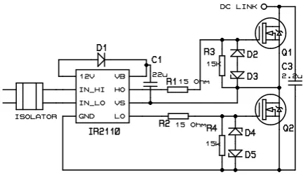
1) MOSFET active rectifier: Fig. 9 shows one leg of
the MOSFET active rectifier. A digital isolator ISO7420FE, IR2110 gate driver and IRFP064N MOSFETs are the key components. The remaining components were selected based on the manufacturer application notes.
The control system comprises of various functional blocks that are explained as follows.
2) ExtendedH∞filter: The extendedH∞filter is a robust
Figure 9: Circuit diagram for the active rectifier - one leg
Algorithm 1 Extended H∞ Filter [19]–[21]
X[k|k−1] = f(x(k), u(k), k)
P[k|k−1] = Φ[k−1]P[k−1|k−1]ΦT[k−1] +Q[k−1]
K[k] = P[k|k−1]HT[k]·
H[k]P[k|k−1]HT[k] +R[k]−1
X[k|k] = X[k|k−1] +K[k] Y[k]−H¯[k]X[k|k−1]
P[k|k] = P[k|k−1]−P[k|k−1]·
HT[k] LT[k] R−1 e [k]·
H[k]
L[k]
P[k|k−1]
Re[k] =
Re11[k] Re12[k] Re21[k] Re22[k]
Re11[k] = R+H[k]P[k|k−1]H
T
[k]
Re12[k] = H[k]P[k|k−1]LT[k]
Re21[k] = L[k]P[k|k−1]H
T
[k]
Re22[k] = −γ2I+L[k]P[k|k−1]LT[k]
whereΦis defined as:
Φ [k] ≈ ∂f(x(k), u(k), k)
∂x
X(k
|k)
The notationΓ [n|m]in Algorithm 1 means the value of the matrixΓat instantntaking into accountmprevious updates. The extended H∞ filter equations were written by using (1) and (2), the speedωmmodelled as a perturbation so that
ωm[k] ≈ ωm[k−1] (5)
and the relationship between the electrical angleθeand the mechanical speed ωm
θe[k] = θe[k−1] +P Tsωm (6)
The corresponding extended H∞ filter equations for the PM generator are written below:
f(x(k), u(k), k) = (7)
(1−RsTs/Ls)id+P Tsωmiq+LTs
sud
−P Tsωmid+ (1−RsTs/Ls)iq−P ωmφLTs
s +
Ts
Lsuq
ωm
P Tsωm+θe
X[k] =
id iq ωm θe
T
(8)
Y[k] =
id iq
T
(9)
H[k] =
1 0 0 0
0 1 0 0
(10)
L =
1 0 0 0
0 1 0 0
(11)
Φ =
1−RsTs
Ls P Tsωm P Tsiq 0
−P Tsωm 1−RLssTs −P Tsid−P TLssφ 0
0 0 1 0
0 0 P Ts 1
(12)
Q[k] = diag 0.05 0.05 0.05 0.015
(13)
R[k] = 0.21×diag(2×2) (14)
γ2 = 0.08 (15)
Q[k],R[k]andγ were tuned according to the application requirements and simulation results.
3) Torque estimator : The estimated load torque TˆL
cor-responds to the wind turbine torque Twind, as a consequence it is unknown and uncontrolled. A Luenberger observer was proposed to calculate TL = Twind. It uses the speed and current to estimate the wind torque.
ˆ
ωm[k+ 1] = ωˆm[k]−
3 2
P Ts
J φiq[k]
+Ts ˆ
TL[k]
J +αL1Ts(ωm[k]−ωˆm[k]) (16)
ˆ
TL[k+ 1] = TˆL[k] +αL2Ts(ωm[k]−ωˆm[k]) (17)
power output of a wind turbine can be written as:
Pm = Cp
ρπr5
2λ3 ω 3
m (18)
whereρis the air density,ris the turbine blade radius,ωm is the rotor speed,Cpis the power coefficient andλis the tip speed ratio defined as:
λ = ωmr
v (19)
v is the wind speed.
Cp andλhave both optimal values that depend on the tur-bine characteristics and are usually provided by manufacturers or estimated from tests (the latter for this paper). The wind turbine emulator test-rig used in this paper has the following mechanical parameters: ρ = 1.225 kg.m−3, r = 0.455 m,
CPopt= 0.25andλopt= 3.75as listed in Table II.
The mechanical torqueT can be written asT =Pm/ωm . In wind turbines, by taking Cpopt,λoptand (18)
T =Cpopt
ρπr5
2λopt3ω 2
opt (20)
Since all the parameters in (20) are constant, for a given torque T, there is an optimal shaft speed ωopt to achieve maximum power extraction. This strategy was used in [9], but the wind torque was measured with a bulky torque transducer. In this paperTis estimated asTˆLusing a Luenberger observer so it can be used to set the optimal speed reference ωopt. To deal with noise, numerical errors and changing wind conditions the following iterative algorithm is proposed:
1) Wait 10 s after the last speed reference update because the system response is relatively slow, compared to a standard PM motor, due to the inertia in the turbine and there is no motoring operation.
2) Take samples of the estimated torque TˆL for 10 s each 0.2 s. Average those samples to get the mean valueT¯L. 3) Calculate the optimal speed reference by using T¯L in
(20) and setωopt as the new speed reference. 4) Return to step one.
5) Further considerations: As already stated, the Rutland
generator is an unbalanced machine and some modifications in the control scheme were required to address this problem. The authors in [16], [17] considered an inverter tied to an unbalanced grid. They addressed the unbalance in the system by using notch filters centred at the grid frequency (50 Hz). This solution cannot be applied in this case because the frequency varies with the generator speed. In this present paper, low pass filters were used to filter out high frequency components due to the unbalance in the generator, but stability problems and reduced bandwidth of the controllers are the drawbacks of this technique. The stability margin decreases if the cut-off frequency is reduced as shown in the next section.
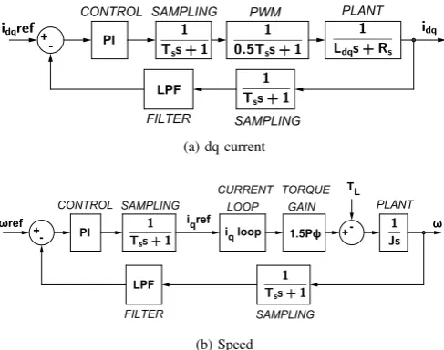
because they are commonly used in wind turbine control, their transfer function is straightforward to write in the Laplace variable and simplifies the stability analysis of the system. Fig. 10a shows the control diagram of the idq currents. The coupling terms in (1) and (2) are compensated using the decoupling termsLqiqP ωmand−LdidP ωm−P ωmφfor the d and q axis respectively. The decoupling terms are directly added to the control voltages feeding the active rectifier. This simplifies the stability analysis and allows evaluating the d
and q axis independently. After the compensation stage, the coupling terms are approximated as disturbances and not included in the block diagram for the stability analysis.
Low pass filters (LPF) were included in the control loop for removing unwanted harmonics from measured signals, especially due to the unbalance in the generator, but these filters also reduced the bandwidth of the controller. A trade-off between stability and performance was necessary. The plant in Fig. 10 was numerically analysed in Simulink using Matlab’s Sisotool toolbox to obtain the Bode diagrams of the system and establish the controller gains using the criteria presented in [25]. Later on, these gains were used as initial values for a detailed simulation implemented in Simulink using its SimPower library. This simulation model included the wind turbine dynamics, estimators and power electronics. The gains obtained with the detailed simulation model were used in the experimental implementation.
TheH∞filter was not included in the stability analysis as it is well known that this filter becomes unstable near zero speed, which is important in motoring mode, but in this application, the generator is started by the blades (prime mover) using passive rectification with the body diodes of the active rectifier to avoid problems at low speed. Also, wind turbines have a cut-in wind speed (around 2.4 m/s) where they start to operate. Near zero operational speeds are therefore unlikely.
Fig. 10b shows the control diagram of the speed. The inner “current loop” block represents the diagram in Fig. 10a for the iq current controller. The load torqueTL was included as a disturbance in Fig. 10b, but it was not considered for the stability analysis.
Discrete time pole-zero maps of the system using different cut-off frequencies for the low pass filters were plotted to explore the stability of the current and speed control loops. The Tustin approximation was used as discretization method withTs= 400 µs.
(a) dq current
[image:8.595.48.292.57.249.2](b) Speed
Figure 10: Block diagrams of the system
the system. It can be also seen that if the cut-off frequency of the low pass filters is reduced, then the dominant poles approach to the border of the unit circle (as indicated by the arrow), therefore the stability margin is effectively reduced. The same behaviour was observed in the pole-zero maps for theidq currents.
Real Axis
Imaginary Axis
−1 −0.5 0 0.5 1
−1 −0.5 0 0.5 1
0.1π/T 0.2π/T 0.3π/T 0.4π/T 0.5π/T 0.6π/T 0.7π/T 0.8π/T 0.9π/T 1π/T
0.1π/T 0.2π/T 0.3π/T 0.4π/T 0.5π/T 0.6π/T 0.7π/T 0.8π/T 0.9π/T 1π/T
0.1 0.2 0.3 0.4 0.5 0.6 0.7 0.8 0.9
[image:8.595.322.536.252.365.2]400 Hz 100 Hz 25 Hz 5 Hz
Figure 11: Pole-zero map for the speed control loop
Real Axis
Imaginary Axis
0.7 0.75 0.8 0.85 0.9 0.95
−0.1 0 0.1 0.2 0.3 0.4
0.1π/T
[image:8.595.312.537.255.525.2]400 Hz 100 Hz 25 Hz 5 Hz
Figure 12: Pole-zero map for the speed control loop - zoomed-in view
VI. EXPERIMENTAL RESULTS
The wind speed profile shown in Fig. 13a was used to initially test the sensorless controller and MPPT algorithm. Fig. 13b shows the speed tracking needed to operate the
turbine near its maximum power coefficient (Fig. 13c) and optimal tip speed ratio (Fig. 13d).
The unbalance between phases is more significant as the rotational speed increases, leading to higher harmonic content in the dq variables, less effective low pass filters and finally the system becomes unstable. The power generation cannot be easily limited since there are no opportunities for yaw or pitch control as is the case in larger wind turbines. The wind speed profile shown in Fig. 14 was applied to the test rig. The steps in wind speed were used to identify the point where system becomes unstable. Fig. 15 shows that the controller was able to track the maximum power point regardless of the wind conditions, up to 14 m/s. The controller was tested with different gains, but the instability point was near 14 m/s in all the cases.
0 100 200 300 400 500
7 8 9 10 11 12 13 14 15
Time (s)
[image:8.595.63.272.385.489.2]Wind Speed( m/s)
Figure 14: Wind speed profile
0 100 200 300 400 500
0 200 400 600 800 1000 1200 1400
Time (s)
Speed (RPM)
Estimation Encoder
Start up
[image:8.595.65.271.545.649.2]Unstable region
Figure 15: Unstable operation
VII. SYSTEM EFFICIENCY COMPARISON
0 100 200 300 400 500 600 6.5
7
Time (s)
(a) Wind speed profile used for MPPT
0 100 200 300 400 500 600
0 200
Time (s)
(b) Speed tracking using MPPT
0 100 200 300 400 500 600
0 0.1 0.2 0.3 0.4
Time (s)
Power coefficient (C
p
)
C pmax=0.25
(c) Power coefficient using MPPT
0 100 200 300 400 500 600
0 1 2 3 4 5
Time (s)
Tip speed ratio (
λ
)
Measurement
λopt=3.75
[image:9.595.55.529.70.341.2](d) Tip speed ratio using MPPT
Figure 13: Sensorless speed control -Experimental results
of the BAS controller is limited to approximately 90 W regardless of the wind conditions. The blue bars are the power coefficient of the turbine directly connected to a lead acid battery. The turbine achieved a higher power coefficient when the battery was close to fully charged as it was shown in Fig. 5, but as already mentioned, the value reported on Fig. 16 corresponds to the average power coefficient. Finally, the green bars correspond to the power coefficient using sensorless control and active rectification. This technique has the highest power coefficient over the range of wind speeds, but the algorithm was stable only up to 14 m/s wind speed.
4 6 8 10 12 14
0 0.05 0.1 0.15 0.2 0.25 0.3 0.35
Wind speed (m/s)
Power coefficient (C
p
)
[image:9.595.50.270.534.647.2]Battery Wind tunnel maximum BAS control Active rectifier
Figure 16: Efficiency comparison
VIII. CONCLUSIONS
The MPPT algorithm, H∞ filter and P I controller de-veloped for small scale wind turbines in [18] were applied to a micro-wind turbine (Rutland 913) intended for battery
charging. The machine parameters of the controller and estim-ation algorithms were changed according to the values of the Rutland turbine. The combination of algorithms and estimators in the sensorless control system for the active rectifier showed fairly good performance up to 14 m/s wind speed, but above this point the system became unstable due to the unbalanced phases of the Rutland turbine. The unbalance in the turbine generator introduced unwanted harmonics in the DC link voltage and phase currents that need to be addressed. Low pass filters were used in this paper, but these filters limited the bandwidth and stability of the controller.
REFERENCES
[1] R. I. of Technology Stockholm-Sweden,Wind Power in Power Systems, T. Ackerman, Ed. John Wiley & Sons, Inc., 2005.
[2] P. Gipe,Wind power Renewable Energy for Home, Farm and Business. Chelsea Green Publishing Company, 2004.
[3] Catalogue of European Urban Wind Turbine Manufacturers, European Commission under the Intelligent Energy Europe programme. [4] Rutland 913 Windcharger Owners Manual, MARLEC, February 2013. [5] AMPAIR 100 Operation Installation & Maintenance Manual
Manufac-tured by Ampair, rev 1.3 ed., Ampair, October 2012.
[6] P. Vas,Sensorless vector and direct torque control, ser. Monographs in electrical and electronic engineering. Oxford University Press, 1998. [7] J. Hendershot and T. Miller, Design of Brushless
Permanent-magnet Machines. Motor Design Books, 2010. [Online]. Available: https://books.google.co.uk/books?id=n833QwAACAAJ
[8] H. Toliyat and G. Kliman,Handbook of Electric Motors, ser. Electrical and computer engineering. CRC Press, 2004. [Online]. Available: https://books.google.co.uk/books?id=4-Kkj53fWTIC
[9] M. Tatlow, “Wind Turbine Emulator System for Testing Small-Scale Wind Generators and Associated Power Electronics,” Master’s thesis, University of Cambridge, 2011.
[10] D. Llano, M. Tatlow, and R. McMahon, “Control algorithms for per-manent magnet generators evaluated on a wind turbine emulator test-rig,” inPower Electronics, Machines and Drives (PEMD 2014), 7th IET International Conference on, April 2014, pp. 1–7.
[11] T. Chen and L. Liou, “Blockage corrections in wind tunnel tests of small horizontal-axis wind turbines,”Experimental Thermal and Fluid Science, vol. 35, no. 3, pp. 565 – 569, 2011. [Online]. Available: http://www.sciencedirect.com/science/article/pii/S0894177710002438 [12] F. Campagnolo, “Wind tunnel testing of scaled wind turbine models:
Aerodynamics and Beyond,” Ph.D. dissertation, Politecnico di Milano, 2013.
[13] M. C. Rose, “Variable speed wind generator control in Antarctica,”
Geophysical Research Abstracts, vol. 9, p. 02051, 2007.
[14] T. Tin, B. K. Sovacool, D. Blake, P. Magill, S. E. Naggar, S. Lidstrom, K. Ishizawa, and J. Berte, “Energy efficiency and renewable energy under extreme conditions: Case studies from Antarctica,” Renewable Energy, vol. 35, no. 8, pp. 1715 – 1723, 2010. [Online]. Available: http://www.sciencedirect.com/science/article/pii/S0960148109004467 [15] D. M. Whaley, W. L. Soong, and N. Ertugrul, “Investigation of
switched-mode rectifier for control of small-scale wind turbines,” inIndustry Ap-plications Conference, 2005. Fourtieth IAS Annual Meeting. Conference Record of the 2005, vol. 4, Oct 2005, pp. 2849–2856 Vol. 4. [16] L. Moran, P. Ziogas, and G. Joos, “Design aspects of synchronous PWM
rectifier-inverter systems under unbalanced input voltage conditions,” in Industry Applications Society Annual Meeting, 1989., Conference Record of the 1989 IEEE, Oct 1989, pp. 877–884 vol.1.
[17] S. Shao, T. Long, E. Abdi, and R. McMahon, “Dynamic Control of the Brushless Doubly Fed Induction Generator Under Unbalanced Operation,”Industrial Electronics, IEEE Transactions on, vol. 60, no. 6, pp. 2465–2476, June 2013.
[18] D. Llano and R. McMahon, “Torque observer and extended H infinity filter for sensorless control of permanent magnet generators tested on a wind turbine emulator,” inIndustrial Electronics Society, IECON 2015 - 41st Annual Conference of the IEEE, Nov 2015, pp. 000 123–000 128. [19] U. Shaked and N. Berman, “H infinity nonlinear filtering of discrete-time processes,”Signal Processing, IEEE Transactions on, vol. 43, no. 9, pp. 2205–2209, Sep 1995.
[20] G. Einicke and L. White, “Robust extended Kalman filtering,”Signal Processing, IEEE Transactions on, vol. 47, no. 9, pp. 2596–2599, Sep 1999.
[21] W. Li and Y. Jia, “H-infinity filtering for a class of nonlinear discrete-time systems based on unscented transform,” Signal Processing, vol. 90, no. 12, pp. 3301 – 3307, 2010. [Online]. Available: http://www.sciencedirect.com/science/article/pii/S0165168410002252 [22] D. Llano, “Sensorless control techniques and associated power
elec-tronics for generators in micro and small-scale wind turbines,” Ph.D. dissertation, University of Cambridge, July 2016.
[23] F. B. Marian Kazmierkowski, R. Krishnan, Ed., Control in Power Electronics. Selected Problems. Academic Press Series in Engineering, 2002.
[24] V. Blasko and V. Kaura, “A novel control to actively damp resonance in input LC filter of a three phase voltage source converter,” in
Applied Power Electronics Conference and Exposition, 1996. APEC ’96. Conference Proceedings 1996., Eleventh Annual, vol. 2, Mar 1996, pp. 545–551 vol.2.
[25] K. Ogata,Modern Control Engineering. Prentice-Hall, 2010.
Danilo X Llanoreceived the BSc. degree in
Elec-tronic Engineering from Universidad San Francisco de Quito, Ecuador, in 2012. He received the Ph.D. degree from the University of Cambridge, UK in July 2016. In October 2016, he joined WMG, at Warwick University, Coventry, UK, as a Research Fellow at the Advanced Propulsion Systems Group. His current research interests includes sensorless control of electrical drives, sensorless estimation al-gorithms, electrical machine and small wind turbine in MATLAB/Simulink, power electronics, wireless instrumentation, electric powertrain systems and sensor design.
Richard A McMahonreceived the B.A. degree in