A housekeeping prognostic health management framework for microfluidic systems

Abstract--Micro-electro-mechanical Systems and microfluidics

are becoming popular solutions for sensing, diagnostics and control applications. Reliability and validation of function is of increasing importance in the majority of these applications. On-line testing strategies for these devices have the potential to provide real-time condition monitoring information. It is shown that this information can be used to diagnose and prognose the health of the device. This information can also be used to provide an early failure warning system by predicting the remaining useful life. Diagnostic and prognostic outcomes can also be leveraged to improve the reliability, dependability and availability of these devices. This work has delivered a methodology for a “lightweight” prognostics solution for a microfluidic device based on real-time diagnostics. An oscillation based test methodology is used to extract diagnostic information that is processed using a Linear Discriminant Analysis based classifier. This enables the identification of current health based on pre-defined health levels. As the deteriorating device is periodically classified, the rate at which the device degrades is used to predict the devices remaining useful life.

Index Terms: Microfluidics, Prognostics and health

Management, Microelectrodes, Design-for-testability, Machine learning algorithms.

I. INTRODUCTION

A novel implementation of a prognostics function for a microfluidic device based on MEMS technology is presented. The term “prognostics” has been defined in various different ways depending on context [1], this research considers the definition given by ISO13381-1 as the most comprehensive. It states that prognostics is not only the prediction of the time to failure but also the risk of one or more existing or future failure modes [2].

Studies have revealed some excellent Prognostic and Health Management (PHM) solutions that provide deep and detailed prognostic capabilities for micro-devices with a high level of accuracy. The use of machine learning [3] and physics based prognostics [4] is being actively explored. PHM solutions

similar to these are designed from the ground up in a device specific framework with the prognostics modules being tightly coupled with the physics of failure of the device. While these PHM systems perform very well in conjunction with their target devices, flexibility and wide scale adoption in other MEMS devices is quite challenging.

The onus of most PHM frameworks is to provide prognosis at the highest possible confidence level thus providing the most reliable Remaining Useful Life (RUL) predictions [5] [6] [7]. However, this comes at a cost, be it a heavy processing requirement or the aforementioned rigidity or complexity, to name two. This work proposes a “Housekeeping” Prognostics and Health Management (HPHM) framework that has a conservative prognostic mandate. Such a framework caters strictly for wear during normal use and evolving faults. This affords the usage of simpler models that are easy to adapt, implement and use.

The scope of this HPHM is to predict patterns of low intensity failures and drift due to gradual aging and non-catastrophic faults during normal operation. The advantages this capability offers is simplicity and speed of adaption with none of the overheads associated with more traditional prognostic methodologies. Furthermore, ease of implementation and cross-device compatibility makes pure hardware realization credible.

II. OVERVIEW

The design and performance of a HPHM solution for a microfluidics based MEMS sensor chip with embedded micro-electrodes is presented in this paper. Such devices are increasingly being engineered for new areas of application. Research is being carried out into embedding microelectrodes directly into human bodies [8] [9] [10] and even into the human brain [11] [12] [13] [14]. Microelectrode based devices are quickly evolving from being temporary and disposable to being devices designed for long term use [15]. The development of a prognostics framework for such devices is relevant given these trends.

For the purpose of this research, experiments have been conducted using a device that is able to mix a reagent and analyte and detect conductivity of the product using embedded electrodes that line the channel.

The proposed prognostics model presented in this work is not a system level solution. It is classified at component level as its focus is limited to the health of the sensing electrodes. The electrodes have been shown to be the most critical components of the microfluidics chip. They have also been shown to be the most vulnerable to failure due to usage and environmental

A Housekeeping Prognostic Health Management

Framework for Microfluidic Systems

H.Khan, Q.Al-Gayem and A.M.Richardson, Member IEEE

Manuscript received January 8, 2017; revised February 26, 2017; accepted April 10, 2017. This work has been funded by Lancaster University, Uk through the Chancellors Scholarship. (Corresponding author: A. M. Richardson.)

H. khan is with the Department of Electrical Engineering, COMSATS Institute of Information Technology, Park Road, Tarlai Kalan, Islamabad 45550, Pakistan. (email: [email protected])

Q. Al-Gayem is with the Electrical and Electronic Department, University of Babylon, Babylon, Iraq. P.O. Box No. 4 Hilla. (e-mail: [email protected]).

A. M. Richardson is with the Department of Engineering, Lancaster University, LA1 4YR, UK. (email: [email protected])

factors. Repeated experiments using similar chips (microfluidic chips with electrodes used for sensing) showed electrode failure to be the largest root cause of system failure in these types of devices followed by blockage and leakage. This is consistent with various other studies available in literature [16] [17] [18] [19].

A diagnostic-prognostics pairing has been proposed for the HPHM:

• Diagnosis: A modified Oscillation Based Testing (OBT) technique has been used to provide real time diagnostics. This forms the input to the prognostics module.

• Pre-prognosis: A machine learning algorithm based on a Linear Discriminant Analysis (LDA) classifier has been used to identify the level of health the sensor is trending towards.

• Prognosis: Periodic health classification is used to process the normal wear and aging trend of the chip. This is used to calculate the RUL.

III. BACKGROUND

Microfluidic devices have distinctive properties when compared to other types of MEMS in the context of reliability, the main difference being the operational load and environmental conditions they are exposed to. There are therefore unique challenges associated with a HPHM framework for these devices.

Applications are wide ranging and include “Lab-on-Chip” devices were there is an increasing interest in MEMS integration due to the improved sensitivity and faster response which have been well documented [20] [21]. Of special interest are technologies capable of integrating microfluidics with electronic sensing, actuation, control and processing. A number of technologies that exist show the capabilities and potential of these integrated chips [22]. With their rapid commercialization, the need for fault tolerant design with integrated health monitoring and health prediction capabilities are gaining traction. The examples quoted here have sensing components and failure modes similar to the MEMS chips used in this study.

This research specifically targets the development of microfluidic MEMS devices with embedded electrodes because there are a number of interesting applications, in addition to those cited above that require the interfacing of microfluidic structures to electronic circuitry [23]. This provides the opportunity for electronic sensing, actuation and processing. The integration with electronics provides a platform for a prognostics processing unit which would not otherwise be possible.

A.Reliability and Failures

The reliability of Bio-MEMS devices is yet to be established as is microfluidics in general that is currently limited in industrial uptake. A number of public bodies are, however, committed to accelerating uptake of these technologies [24].

Failures in Microfluidic devices have been identified to be unique [25] due to direct contact of their components with fluids, i.e. liquid bio-chemical assays. In addition to

degradation due to direct contact, failure mechanisms including blockages and fouling are significant and sensitive to the density and/or viscosity of the liquids. The chip used in this research demonstrated two levels of failure;

• Blockage of and sedimentation on the electrode surface.

• Deterioration and aging due to normal use.

IV. FAULT MODEL

Electrode degradation causes significant loss in monitoring ability, especially in MEMS device based sensing of cellular level specimens. The development of embedded test methods based on OBT [26] [27] forms an important contribution to the prognostic methodology proposed. The experiments conducted in this research validated the premise that the electrodes are the key target for a first-generation prognostics solution for electrode based microfluidics.

A.Embedded Electrodes – Failure Mechanisms and Failure

Modes

Electrode failure involves either:

• Catastrophic Failure (leading to complete loss of operational functionality).

• Gradual Degradation causing a deviation in normal parameter drift associated with operational wear and tear.

Three main fault mechanisms have been observed in the electrodes of the MEMS chips that were used in this work. They are:

• Degradation due to surface material loss. This is due to ion loss in the mixture that surrounds the electrodes. • Settling and sometimes scaling of bio-chemical matter on the electrode surface that is not always removed by cleaning.

• Minor damage due to the cleaning process. Ideally, the electrode structures should be cleaned immediately after every test cycle because residual bio-chemical specimens may be impossible to remove after a delay due to electrolyte evaporation.

The failure modes associated with the electrodes after degradation:

• Marked increase in the impedance / decrease in admittance of the electrode.

• A fluctuation in the bio-fluidic interface capacitance of the electrode.

• A reduction in the Signal to Noise Ratio (SNR) in the signal extracted from the electrodes.

V. OSCILLATION BASED TEST (OBT) DIAGNOSTICS The proposed HPHM framework consists of two subcomponents as described in section 2, i.e. the OBT self-test based diagnostics and the LDA based prognostics. The output of the diagnostic forms the input to the prognostics module. This section will discuss the diagnostics in some detail.

In OBT, the system being tested is designed to operate at specific oscillation frequencies. This oscillation frequency is a function of the material properties and physical structure of the system. Faults can be identified because they cause a deviation in the oscillation frequency from its nominal value. One of the earlier adaptions of this method to test analogue integrated circuits was presented by B Kaminska et al [28]. The validity of this technique has been verified as a test method for operational amplifiers and analogue to digital converters.

The authors of this paper previously demonstrated a scheme for effective degradation monitoring of electrodes within microfluidics systems using OBT [26] [27]. The solution was based on fault modelling and impedance analysis of the interface between the electrode and the electrolyte. The method has also been evaluated within a MEMS based system through work on a monolithic magnetometer [29]. The potential for using OBT in a DNA sensor array has also been researched [30] where both the sensing and test modes can be realised in an oscillation based structure. Some DNA sensors that employ micro-electrodes are similar to the chip used in these experiments. The potential of OBT in such DNA sensors has been explored [31]. It has been observed that normal sensing operation results in the hybridized DNA strands deposited on the electrodes causing the displacement of ions from the surface which results in a considerable change in the interface capacitance of the electrical double layer. OBT converts this varying capacitance to a frequency as a means of testing the integrity and state of operational health of the electrode.

A.Experimental Setup

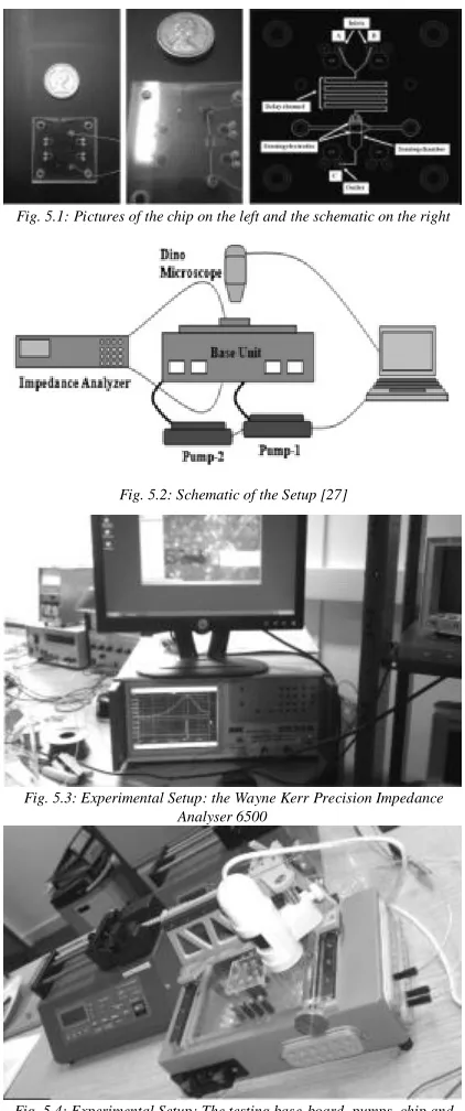
The experiments to extract health data from physical devices were based on microfluidic mixing chips using electrode based sensing. A picture and a schematic of one such chip is shown in Fig 5.1. Two liquid specimens are pumped into the chip which are mixed in the mixing chamber. The resultant electrolyte is analysed via electrolysis when the solution is exposed to a pair of electrodes lined within the outgoing microchannel.

The experiments utilised a microfluidic platform which can be used to demonstrate a number of sensing, mixing and separating experiments, a schematic of which is shown in Fig 5.2 and pictures of which are shown in Fig 5.3 and Fig 5.4. The setup consists of a base board that can host the chip via connectors and fluidic interfaces. Standard lithographic and machining processes have been used to etch the micro channels in both the chip and the base-board that are constructed of Poly-methyl methacrylate (PMMA), acrylic glass and SU-8 photoresist.

The platform consists of a pair of microfluidic precision pumps, an impedance analyser, base-board mounted microscope as well as the control software. The pumps can

control the bi-directional flow rate of the liquids accurately and quantifiably down to the -meter per minute flow rate.

Fig. 5.1: Pictures of the chip on the left and the schematic on the right

Fig. 5.2: Schematic of the Setup [27]

Fig. 5.3: Experimental Setup: the Wayne Kerr Precision Impedance Analyser 6500

Fig. 5.4: Experimental Setup: The testing base-board, pumps, chip and digital microscope

injection into the sensing chamber. The Channel is 150 m wide and 75 m deep. The total length of the DC is 9 cm. A channel length above 1 cm in a mixing chamber with the dimensions used here to induce turbulence is considered to be sufficient to ensure a mixing index of above 0.95 [34], even for low Reynolds number (≥1). During experiments, mixing efficiency was observed to be above 90% at 1 L/min flow rates which dropped to below 50% at 6 L/min. The total volume of the DC is approximately 1.0124 L.

The sensing chamber has been fabricated with two Nickel electrodes with two arms each, one on top of the other. The electrode arms are 0.25 mm thick and 2.15 mm long. They overlap each other with a distance approximating the height of the chamber. The SC is as deep as the DC but is 2.35 mm wide and 5 mm long.

A software controller written in LABVIEW is used to control the flow of the reagents. The precision pumps connected to the PC serially via RS232 interface are controlled using this software controller. The software controller can control the pumps individually. Based on the flow orientation required and diameter of the reagent filled syringes that are used to feed the pumps, different flow rates can be maintained on each individual pump.

The experiment involves pumping in 0.1 M NaOH at an infusion rate of 1 L/min throughout the test at room temperature. The second pump introduces 0.1 M HCl at initially 0.1 L/min, gradually increasing at discrete intervals until matching the flow rate of NaOH. This is done to ensure that the HCl solution does not contaminate the sensing chamber. These flow rates were chosen to ensure optimal mixing of the reagents in the DC. This was validated by introducing solutions into the chip with coloured agents and observing their diffusion visually under the microscope.

Experiments were designed to conclude after a maximum of 5 hours. Healthy chips are exposed to multiple cycles, with a cleaning session preceding each test cycle. It has been observed that the electrical characteristics of the Nickel electrodes start deviating from expected behaviour after the 3 hour mark of the first cycle, indicating a deterioration of the electrode surface.

The objective of the experiment is to test the conductivity of the resulting fluid at different flow rates and sensing its composition based on its electrical properties. The measurements are observed directly from a Wayne Kerr Precision Impedance Analyser 6500 that is connected to the electrodes. As mentioned before, the flow rates are controlled using the LABVIEW controller, though they can also be manipulated directly on the pumps, albeit, with a lesser degree of sensitivity.

B.Results & Observations

The primary objective of the experiments was to generate data to train and test the prognostics module. For this purpose, the experiments were designed keeping the needs of the prognostics module in mind. This is reflected in the discussion about the experimental stages as follows:

1)Experimental Stages

The prognostics solution uses machine learning engines. A machine learning classifier needs to be trained using experimental data and needs to be experimentally tested after it is trained. Consequently, the experiments were divided into two similar but distinct phases, namely;

• Training Data Collection: Diagnostic data was generated by OBT. This was a set of parameters representing the known health of electrodes at various stages of degradation and aging. This data was then used to train a number of supervised machine learning classifiers. Based on this training, the prognostics system is able to compute the health of the electrodes and over a period of time (typically 5-10 cycles of observation) to predict the RUL of the system based on its current and historical health status. The frequency of these observations depends on the volatility of the system under observation. The prognostics module presented in this research has been discussed in detail in section 6.2. The training depends on but is not limited to:

o The design of the fault model and identification of the most significant parameters.

o The quality and reliability of data.

o The volume of the data.

• Testing: Here, healthy chips were again used to take measurements on the solution while known patterns of operational wear and aging were simultaneously applied to the electrodes. In this round of experiments, the wear predictions of the “trained” system were observed and compared with the “actual” wear of the electrodes.

The experiment utilised a 50 mV electrode stimulus at the 1 KHz and 50 MHz frequency ranges. Hundreds of readings were observed and recorded for the mixing for a range of flow rates that were increased in discrete steps. The flow rate is important as the speed of the fluid flow has a bearing on the quality and consistency of product. The rate of flow should be sufficiently slow for proper mixing to take place before the mixture passes the electrode. This is due to the low Reynolds numbers involved and the dominance of diffusion in the mixing process given laminar flow.

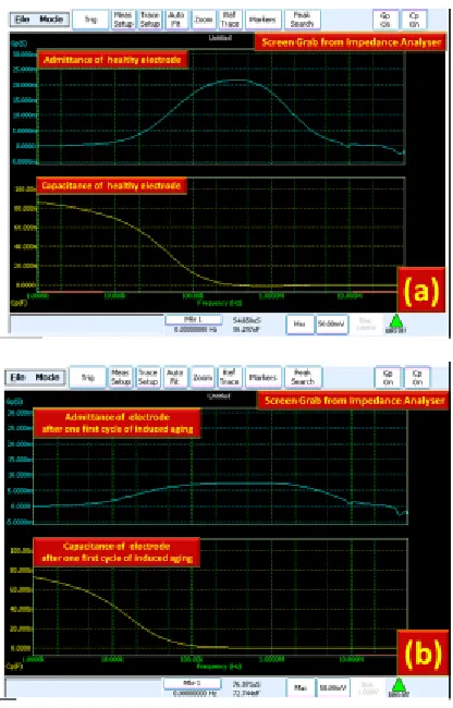
Fig. 5.5: [Impedance Analyser screen-grab] (a) Shows an output for a healthy electrode, where the blue curve is the admittance and the yellow curve is the capacitance of the electrode. (b) Shows the same electrode after induced aging. The change in both the admittance and capacitance is evident

This experiment was repeated over a batch of chips. Data in excess of 32 thousand samples was gathered. That volume of data was calculated to be reasonably sufficient for the effective training of the offline system.

2)Data Analysis

OBT was used to extract the following three electrical parameters (1 input and 2 output parameters)

• Frequency (Hz) – (input) • Admittance (S) – (output) • Capacitance (F) – (output)

The mechanical deterioration of the electrodes manifested in changes in these electrical properties. This is evident from two sets of observations seen in Fig 5.5 and two overlapped observations seen in Fig 5.6. These are actual screenshots captured from the Wayne Kerr Precision Impedance Analyser 6500.

A closer look at the shorter ranges for admittance and capacitance can be seen in Fig 5.7 and Fig 5.8 respectively. Each of these figures shows observations at 4 different levels of health. These 4 levels of health formed the basis of the 4-class health classifier that the prognostics module uses to identify levels of health and their rates of deterioration.

Fig. 5.6: [Impedance Analyser screen-grab] This is a superimposed (held) observation of the same electrode at two different level of health. The graph

is showing both the admittance (left blue y-axis) and capacitance (right yellow y-axis) over a frequency range. The change in both admittance and capacitance is evident from the observations. Similar observations allowed

us to limit the experiments to a narrow band of frequencies where these changes were most significant.

Fig. 5.7: Sample Admittance at different levels of health over the selected frequency range (Dark-blue:1, green:2, red:3 and light-blue:4)

Fig. 5.8: Sample capacitance at different levels of health over the selected frequency range (Dark-blue:1, green:2, red:3 and light-blue:4)

VI. PROGNOSTICS

The prognostics module comprises of two algorithms: • The first algorithm is the classifier that identifies the

current health of the system in quantifiable terms. • The second algorithm uses the series of classifier

no conceivable scenario where the health of the electrode would ever improve).

•

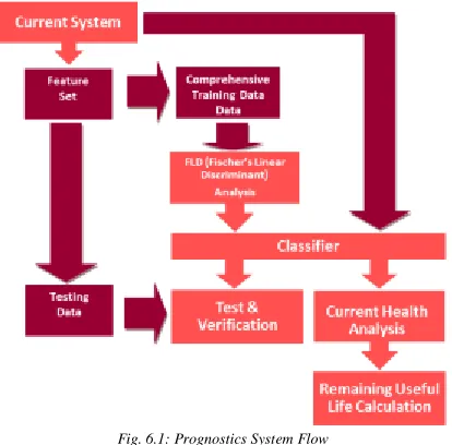
A summary of the life cycle of a generic prognostics system is given in Fig 6.1.

A.The LDA based classifier

In the previous section, we have seen that the OBT is able to convey reliable data about the capacitance and conductance across electrodes at given frequencies. This information cannot be used in isolation as the capacitance or conductance at any given frequency also depends on the constituency and the flow rate of the fluid. In this work, this quantification has been achieved using a classification technique.

Fig. 6.1: Prognostics System Flow

Classification techniques have been extensively used in the areas of machine learning and statistics. These techniques have found wide range of usage in the field of information technology, specifically in the areas of pattern classification and image recognition [35]. Many such techniques have matured over time and are currently industry standards and are known as classifiers.

Linear Discriminant Analysis (LDA) is one well established classification technique. LDA has found application in the areas of banking, financial market predictions, face recognition and studies of epidemiological trends [36] [37] [38]. The basic idea of an LDA classification is to find a transformation for a sample of features that allows for a linear discrimination between classes. Generally speaking, any classifier is an algorithm that is able to distinguish and classify an entity based on certain features. In the context of the sensor under study, electrodes can be classified in terms of their health “class”, from within a set of predefined discrete health classes. Health determining features need to reflect the device health. As indicated in the previous section, the features in this study are frequency, capacitance and conductance.

Even though LDA are traditionally binary classifiers (i.e. they can be used to differentiate between two classes only), they have evolved to accommodate multi-class identification. Literature, especially that pertaining to pattern recognition has

firmly established that the LDAs can easily be extend to a multi-class cases [38] and have been successfully used in many recognition tasks [39].

Fisher’s LDA (FLD) [40], which produces discriminative feature transforms as a set of eigenvectors, is an established standard in the domain of pattern recognition. FLD can be easily extended to multi-class cases via multiple discriminant analysis [41]. In fact, discriminant analysis has been widely used in this way in pattern recognition problems, and its use in reducing facial recognition problems is well documented [42]. This has been the motivation to use discriminant analysis for multiple distinct binary classifications.

LDA is a “supervised learning” classification technique. This implies that the system has to be trained under “supervision” to “learn” how to distinguish between classes. This process is known as training and is a critical part of LDA. The quality and comprehensiveness of training data can affect the quality of performance (class identification).

A collection of feature samples representing known values of health are used as training data. Ideally, all classes of health are represented comprehensively. For the initial tests, 4 levels of electrode health were defined. The 4 classes being:

1. Healthy - health level 1

2. Somewhat healthy - health level 2 3. Somewhat sick - health level 3 4. Sick - health level 4

Although these 4 levels of health have been chosen for this demonstrator, the system can be scaled to accommodate finer degrees of health.

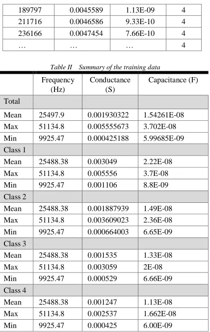
A batch of chips were tested at different (four) levels of electrode health. The corresponding values for frequency, capacitance and conductance for each observation were logged. A total of 32000 samples of known health were collected. Subsets of this data were used for both training and validation of the system. A subset of the actual “training data” can be seen in Table I. A summary of the “training data” set is shown in Table II. The training data consists of data collected for known health at different flow rates and fluid concentrations. The behavioural input allows the classifier to correctly identify levels of health at the flow rates and concentration levels at which the data was generated.

Table I Training Data Sample Subset

Frequency (Hz)

Conductance (S)

Capacitance (F)

Health

… … …

109892 0.0071345 2.95E-09 1

122583 0.0072786 2.42E-09 1

136740 0.0074053 1.97E-09 1

152532 0.0075154 1.59E-09 1

12213.7 0.0046113 2.27E-09 2

… … … …

… … … …

122583 0.0050376 2.02E-09 3

152532 0.005246 1.37E-09 3

170147 0.0053308 1.11E-09 3

189797 0.0045589 1.13E-09 4

211716 0.0046586 9.33E-10 4

236166 0.0047454 7.66E-10 4

… … … 4

Table II Summary of the training data

Frequency (Hz)

Conductance (S)

Capacitance (F) Total

Mean 25497.9 0.001930322 1.54261E-08 Max 51134.8 0.005555673 3.702E-08 Min 9925.47 0.000425188 5.99685E-09 Class 1

Mean 25488.38 0.003049 2.22E-08 Max 51134.8 0.005556 3.7E-08 Min 9925.47 0.001106 8.8E-09 Class 2

Mean 25488.38 0.001887939 1.49E-08 Max 51134.8 0.003609023 2.36E-08 Min 9925.47 0.000664003 6.65E-09 Class 3

Mean 25488.38 0.001535 1.33E-08 Max 51134.8 0.003059 2E-08 Min 9925.47 0.000529 6.66E-09 Class 4

Mean 25488.38 0.001247 1.13E-08 Max 51134.8 0.002537 1.662E-08 Min 9925.47 0.000425 6.00E-09

A scatter plot of the training data can be seen in Fig 6.2. Even though we can see a fine separation in the data at different levels of health, we can see in Fig 6.3 there is an overlap between health levels. The LDA seeks to:

• Further increase the separation between the classes. • Reduce the dimension of the feature set for ease in

prognostics computations.

A number of LDA classifiers were trained using subsets of the master training data. Other subsets from within were used to validate classification performance.

The following section details the training process. An evenly distributed subset of 1000 samples was used for one training session (n = 1000). The samples were divided evenly to represent each class (i.e. 250 samples for each health level, ordered by the health, as seen in Table I)

The matrix for the samples is represented as X and the corresponding health values by the matrix H in the following expression:

𝑋 = [

𝑥1𝑓𝑟𝑒𝑞𝑢𝑒𝑛𝑐𝑦 ⋯ 𝑥1𝑐𝑎𝑝𝑐𝑖𝑡𝑎𝑛𝑐𝑒

⋮ ⋱ ⋮

𝑥1000𝑓𝑟𝑒𝑞𝑢𝑒𝑛𝑐𝑦 ⋯ 𝑥1000𝑐𝑎𝑝𝑎𝑐𝑖𝑡𝑎𝑛𝑐𝑒

] , 𝐻 =

































4

...

...

1

1

Fig. 6.2: 3D Scatter plot of raw data samples collected at different stages of induced (and known) aging, red being healthy and cyan being

the least healthy from the group

Fig. 6.3: Zoomed in view of the 3D scatter matrix in Fig 6.2. Even though the data is quite clean for raw data, 100% separation is not

attainable as evident from the graph.

Where H is a [1x1000] matrix corresponding to the 1000 known samples used in one training session. The typical data in matrix X is derived from the master sample space which has been summarized in Table II.

The first step was the calculation of means of all the features w.r.t classes i.e. means of all values of x for frequency at health 1 … health 4 individually, and so on for the rest of the features.

𝑚_𝑖= [ 𝜇_{𝜔𝑖 (𝑓𝑟𝑒)} 𝜇𝜔𝑖 (𝑐𝑜𝑛)

𝜇𝜔𝑖 (𝑐𝑎𝑝)

] 𝑤ℎ𝑒𝑟𝑒 𝑖

= 1, 2, 3, 4 (𝑡ℎ𝑒 𝑐𝑙𝑎𝑠𝑠𝑒𝑠 𝑜𝑓 ℎ𝑒𝑎𝑙𝑡ℎ)

In the above expression, mi is the mean vector. The contents of this matrix are referenced in Table II.

1)LDA Training

At this point we are ready to train the data. As we are using FLD, we are expecting a transformation with the following outcome:

• A scatter matrix which allows linear discrimination between classes.

• Information about possible dimensionality reduction i.e. identification of features that do not have significant say in classification. These features can be disregarded in the actual classification.

FLD requires us to compute two kinds of matrices, namely; the within-class (SW) and inter-class (SB) scatter matrices.

The within-class (SW) scatter matrix is computed as follows:

𝑆𝑊= ∑ 𝑆𝑖 𝑤ℎ𝑒𝑟𝑒 4

𝑖=0

𝑆_𝑖= ∑ (𝑥 − 𝑚_𝑖)(𝑥 − 𝑚_𝑖)𝑇 250

𝑥∈𝐷𝑖

Which is calculated for all features within each class individually using the relevant value of 𝑚_𝑖 computed earlier. In our case, the Sw was a [3x3] matrix.

The [3x3] inter-class (SB) scatter matrix is calculated as follows:

𝑆_𝐵 = ∑4 250

𝑖=0 (𝑚𝑖− 𝑀)(𝑚𝑖− 𝑀)𝑇 𝑤ℎ𝑒𝑟𝑒

𝑀 𝑖𝑠 𝑡ℎ𝑒 𝑡𝑜𝑡𝑎𝑙 𝑚𝑒𝑎𝑛 𝑓𝑜𝑟 𝑎𝑙𝑙 𝑐𝑙𝑎𝑠𝑠𝑒𝑠

The matrix A is calculated using the SW &SB matricies as

follows:

𝐴 = 𝑆𝑊−1𝑆𝐵

The eigenvectors and eigenvalues for matrix A are defined by the following expression:

𝐴𝑣 = 𝜆𝑣 𝑤ℎ𝑒𝑟𝑒 𝑣 = 𝐸𝑖𝑔𝑒𝑛𝑣𝑒𝑐𝑡𝑜𝑟

𝜆 = 𝐸𝑖𝑔𝑒𝑛𝑣𝑎𝑙𝑢𝑒

2)Feature Reduction

The Eigenvectors and their eigenvalues are used to project the data into a new feature subspace. The resulting new feature subspace separated the health classes very cleanly.

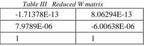
It is important to note that eigenvectors with the lowest eigenvalues bear the least amount of information about data distribution. Any eigenvector with an eigenvalue significantly smaller than other eigenvalues can be ignored with minimal effect on the classification. In our experiments, one eigenvector had a significantly lower eigenvalue (close to 1% compared to the first and the second). This allowed us to drop this feature and use a simpler feature set for our classification. After dropping the third eigenvector, we were able to make our reduced [3x2] transformation matrix W. The resulting reduced W matrix can be seen in Table III.

Table III Reduced W matrix

-1.71378E-13 8.06294E-13 7.9789E-06 -6.00638E-06

1 1

At this point we were able to derive our trained classifier Y with the following expression:

Y = X.W

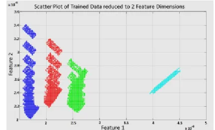
Y is the [1000x2] weighted matrix that will be used to classify any incoming data. The scatter plot of the Y matrix can be seen in Fig 6.4. The stated objectives for the classifier were a reduction in feature dimension and an increase in data separation. It is evident from the figure that these objectives have been achieved.

Table IV Summary of reduced Y-Matrix reduced to two feature dimensions. Total number of determination sets 16000, with 4000

representing each class (1-4)

Feature 1 Feature 2 Total

Mean 2.65E-08 2.44E-08

Max 4.51E-08 3.84E-08

Min 1.55E-08 1.51E-08

Class 1

Mean 4.22E-08 2.44E-08 Class 2

Mean 2.56E-08 2.42E-08 Class 3

Mean 2.11E-08 2.46E-08 Class 4

Mean 1.69E-08 2.44E-08

In this particular instance, a level of separation has been achieved where feature 2 can be discarded without compromising the performance of the classifier. The decision to discard a feature as such can only be made after the extra features have been reduced by the feature reduction algorithm. In this case, the resultant classes can be identified using feature 1 alone. However, this is often not the case.

3)Classifier Usage

Input to the prognostics engine is a vector with three values corresponding to the chosen feature set, i.e. frequency, capacitance and conductance (X’). The sample is transformed into the reduced feature space by computing a dot product with the W matrix (Table III) after subtracting the (total) mean matrix M from it. We obtain the transformed Y’’ as follows:

X”= X’-M (where M is the total mean) Y”= X”.W

Y” is a [1x2] matrix representing a point in a two dimensional plane representing the sample to be classified.

The Euclidian distance between Y” and the mean of each class is measured to determine which class X’ belongs to.

A number of samples with known levels of health are fed to the classifier. The classification output is compared to their actual health to validate the performance of the classifier. This is discussed in some detail in the next section.

4)Classifier Validation

The measure of confidence in a classifier is the ratio between the “true positives” with the “false positives”.

testing sample was also part of the input. i.e. the class (health) of the testing samples is known. This is the reference for comparison to the classifier output. The performance of the classifier has been represented in the form of a confusion matrix shown in Table V. This is a map comparing input health (Actual <class>) to classifier output (Predicted <class>).

Table V Confusion Matrix for one instance of a 1000 sample validation matrix

N=1000 Predicted 1 Predicted 2 Predicted 3 Predicted 4

Actual 1 249 1 0 0

Actual 2 1 247 2 0

Actual 3 0 2 242 6

Actual 4 0 0 7 243

The job of the classifier is to assign every test sample to the correct class. If a sample that belongs to class C is assigned class C, the event is known as a “true positive” (TP) with

Fig. 6.4: The trained data that has been reduced to 2 Feature Dimensions shows a clear separation between classes of health. The right most (cyan) representing health-1

to the left most (blue) representing health-4. This is a representation of the final 16000 sample classifier output.

respect to C. False positives (FP) with respect to C are the samples that are assigned to C but in fact, belong to another class. The corresponding True Positives (TP), True Negatives (TN), False Positives (FP) and False Negative (FN) scores are given in Table VI.

Table VI Class prediction confidence matrix

Class 1 Class 2 Class 3 Class 4

TP 249 247 242 243

TN 749 747 741 744

FP 1 3 9 6

FN 1 3 8 7

The accuracy of the classifier is the percentage of correctly predicted labels divided by all predictions. Two further measures to evaluate classifier performance are precision and recall.

Precision for a class C can be represented as:

𝑝𝑟𝑒𝑐𝑖𝑠𝑖𝑜𝑛_𝐶 = 𝑇𝑃𝐶

𝑇𝑃_𝐶+ 𝐹𝑃_𝐶

𝑝𝑟𝑒𝑐𝑖𝑠𝑖𝑜𝑛_𝑐 = 𝑇𝑃𝑐

𝑇𝑜𝑡𝑎𝑙 𝑝𝑟𝑒𝑑𝑖𝑐𝑡𝑒𝑑 𝑡𝑜 𝑏𝑒 𝑜𝑓 𝐶

While the recall for a class can be represented as:

𝑟𝑒𝑐𝑎𝑙𝑙𝐶 = 𝑇𝑃_𝐶 𝑇𝑃𝐶+ 𝐹𝑁𝐶

𝑟𝑒𝑐𝑎𝑙𝑙_𝑐 = 𝑇𝑃𝑐

𝑇𝑜𝑡𝑎𝑙 𝑎𝑐𝑡𝑢𝑎𝑙𝑙𝑦 𝑏𝑒𝑙𝑜𝑛𝑔𝑖𝑛𝑔 𝑡𝑜 𝐶

The average accuracy of the LDA classifier across all classes for this validation test was found to be 98.1%. Similarly the average precision and recall were also 98.1%. A number of validation runs provided similar classification performance. Even as the number of test samples was increased to 16000 (with uneven class distribution), none of the performance variables went below 95%.

5)Conclusion

So far, a 4 (health) class system has been discussed. In later experiments the number of classes was increased to 16 levels of health. It was observed that the system input had to be restricted to a shorter spectrum and at a higher resolution to achieve an acceptable level of separation between features identifying the classes. Consequently, the average accuracy of the classification deteriorated to 82.61%.

A variety of robust and mature methodologies for classifications and feature reduction are being used in various fields today. These experiments serve to present the potential to identify the health of a device using one such technique. This research presents the idea that classification methods can be used to facilitate the automatic diagnosis and prognosis of components under test using a programmable chip.

B.End of Life Predictor

The classification data was used to identify the health of the electrodes as they changed. This change in the health was logged over time and a quadratic linear algorithm was applied to predict the prognostic data. This data was compared with a predefined “total failure” threshold. Based on the rate and amount of change, the system was able to make predictions about the remaining useful life of the system within a reasonable horizon.

In normal operation, a periodic OBT self-test is initiated. Each iteration of this test generates a data set consisting of values for input: frequency, capacitance and conductance. This is reduced to a [1x2] matrix using the W matrix in Table III. The resulting Y” value is analyzed against the means of the 4 individual health classes of the classifier data. This classifier data is the reduced 2 feature data set summarized in Table IV. The Euclidean distance(s) between the observed sample and mean of each class is measured. The sample is labelled to the class whose mean the sample is at the minimum distance to. All the analytical data of interest is logged at every point of observation. This includes, but is not limited to:

• The reduced 2 feature set of observed data • The assigned class of the observed sample

• The Euclidean distance(s) between the sample and mean of each class

• The percentage distance between the two nearest classes, relative to the nearest class (dn being the distance from the nearest class and ds that from the second nearest). governed by the following expression:

o 𝑃 = ( 𝑑𝑛

The prognostic module has been designed for a two feature system. This program has access to the observations that are logged. This log of observed and processed data forms the basis of the quadratic predictor at the heart of the prognostic engine. In its current version, the prognostics engine observes samples every 10 clock cycles and does not start to operate before the first 50 clock cycles (5 cycles of observation). As the system deteriorates, the sample moves from better health, to worse. This is reflected in subsequent observations and their distances from class means available in the log.

The module subjects the observed values to quantized normalization to bring them in alignment. Each adjusted observation 𝑃𝑛 can be represented as follows:

𝑃_{𝑛= 𝐶 − 𝑡 + √((𝑃 100}⁄ ) − 𝑡)2

Where

C = assigned class P = percentage distance

t = trend {0 𝑖𝑓 𝑜𝑏𝑠𝑒𝑟𝑣𝑎𝑡𝑖𝑜𝑛 𝑙𝑒𝑎𝑛𝑠 𝑡𝑜 𝑎 ℎ𝑒𝑎𝑙𝑡ℎ𝑖𝑒𝑟 𝑐𝑙𝑎𝑠𝑠_{1 𝑖𝑓 𝑜b𝑠𝑒𝑟𝑣𝑎𝑡𝑖𝑜𝑛 𝑙𝑒𝑎𝑛𝑠 𝑡𝑜 𝑢𝑛ℎ𝑒𝑎𝑙𝑡ℎ𝑦 𝑐𝑙𝑎𝑠𝑠}

0 ≤ 𝑃𝑛≤ (max(𝐶 𝑣𝑎𝑙𝑢𝑒) + 1)

In the 4-class paradigm, the prognostic program filters out any value above 4 by default. Any 𝑃_𝑛value above 4 represents an event past system failure, and is hence, useless.

The 𝑃𝑛 values always move from their first observation

towards 4 as the device ages and performance degrades. As successive changes in health are stored, this historical data is used to derive a health trend over time (observation cycle numbers), which in turn is extrapolated to predict the time when the system will reach total failure. The point of observation where 𝑃_𝑛 crosses 4 is considered to be the time of actual failure.

Several tests were performed to test this algorithm and the health predictions at various points were observed. These were then compared to eventual points of failure. An example of some failure predictions over a sequence of tests for a system which was artificially and drastically aged are shown in Table VII.

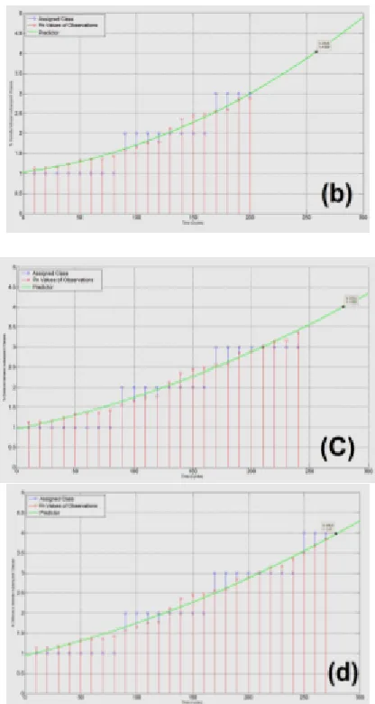
Data generated from the program has been imported to MATLAB to produce the graphical representations shown in Fig 6.5.

Fig. 6.5: Each graph is representing the Pn values of each observation (red

dot), the corresponding class assignments (blue dot) and the predictor (green curve) that is used to identify predicted End of Life (EoL). The diagrams

represent observations at

(a) 150 cycles where the EoL prediction is the 215.2 cycle mark (b) 200 cycles where the EoL prediction is the 258.6 cycle mark (c) 240 cycles where the EoL prediction is the 278.8 cycle mark and (d) 270 cycles where the system is about to

fail

Table VII End of Life (EoL) predictions at various points of Prognosis

Cycle of prediction Predicted EoL

150 218.18

200 258.60

240 278.78

270 278.78

In the example that has been presented, the electrodes were aggressively aged. Normal prognostics tests were performed over a significantly larger volume of data.

These experiments present a blueprint laying out the foundations for the development of a prognostics system for a MEMS device. The algorithm is scalable enough to be refined to provide prognostics over larger horizons with minimal overhead.

to a potential for the system to be realized for embedded systems. However, this system operates based on the assumption that the health will only deteriorate. This suits the mandate of a “house-keeping” prognostics framework.

Over the course of numerous tests on the chips, the prognostics module achieved an average accuracy of next class prediction with over 98% accuracy and an EoL prediction with over 99% accuracy at a prognostic horizon of 100 cycles of observations (1000 clock cycles). The EoL prediction held this accuracy only for gradual deterioration which is consistent with wear in normal operation and aging.

VII. CONCLUSION

The principle outcome of this research is a proof of concept design for a housekeeping prognostics health management solution for MEMS sensors. This is significant as there is very little published work that provides health prediction for MEMS devices.

This work has introduced the concept of “housekeeping” prognostics. The “housekeeping” paradigm has conservative accuracy to enable its realization in a resource constraint framework common to MEMS. At the same time it delivered the potential for an unprecedented reduction in maintenance overheads. This research validated the viability of integrating prognostics in MEMS by demonstrating the use of simplified statistical prognostics techniques in MEMS sensors in the case study presented. While the techniques applied are well established in the fields of finance, computing and image processing, they had not been used to predict the future health trends in MEMS artefacts before.

In the case study, systems were tested using experiments that gradually aged embedded electrodes (being the single most critical components of the MEMS sensor under test). The usage degradation and aging processes were electrically self-induced and controlled. The decay process represented a gradual drift in health as the prognostic system was designed to detect and predict a deterioration of this nature. This is satisfactory as far as the requirements of a “housekeeping” prognostics module are concerned. The consequent light weight processing allowed for the integration of such housekeeping PHMs at a relatively low overhead. However, the PHM is not designed to predict sudden and catastrophic failures.

It was observed that the PHM was consistent with its requirements and design, i.e. while it was able to predict the RUL with gradual aging and drift due to failure; it was unable to respond or detect abrupt or rapid failures. The prognostics module predicted the projected levels of gradual aging of the electrode sensors after 5 cycles of observation (50 clock cycles) with good accuracy.

The challenge of meaningful identification of electrode health was successfully achieved using LDA classifiers with minimal overlaps. The log of this health data formed input to the Linear Predictor that was able to predict the future health of the system.

The scope of this PHM is aging and does not cater for systems that are susceptible to sudden failures leading to critical

faults. This research proposes the use of these “intermediate-level” prognostic capabilities that may not be fully featured as more complex PHM systems but still provide a significant advantage in the reliability and maintenance of MEMS devices. These experiments open up the possibilities to study patterns of abnormal behaviour to predict reliability based on anomalous health patterns. This is critical for systems that may functionally be in a state of degradation without triggering the flags or markers that identify a system to be progressing towards a fatal state.

VIII. REFERENCES

[1] J. Sikorska, M. Hodkiewicz and L. Ma, “Prognostic modelling options for remaining useful life estimation by industry,” Mechanical Systems and Signal Processing, vol. 25, pp. 1803-1836, 2011.

[2] D. A. Tobon-Mejia, K. Medjaher and N. Zerhouni, “The ISO 13381-1 standard's failure prognostics process through an example,” in Prognostics and Health Management Conference, 2010.

[3] Q. K. O. Al-Gayem, “Test and Condition Monitoring Technologies for Bio-fluidic Microsystems,” PhD, Engineering, University of Lancaster, 2012.

[4] C. S. Kulkarni, “"A physics-based degradation modeling framework for diagnostic and prognostic studies in electrolytic capacitors,” Vanderbilt University, 2013.

[5] S. Mathew, M. Alam and M. Pecht, “Identification of failure mechanisms to enhance prognostic outcomes,” Journal of Failure Analysis and Prevention, vol. 12, pp. 66-73, 2012. [6] P. Lall, R. Lowe and K. Goebel, “Extended Kalman filter models

and resistance spectroscopy for prognostication and health monitoring of leadfree electronics under vibration,” IEEE Transactions on Reliability, vol. 61, pp. 858-871, 2012. [7] T. Sutharssan, S. Stoyanov, C. Bailey and Y. Rosunally,

“Prognostics and health monitoring of high power led,” Micromachines, vol. 3, pp. 78-100, 2012.

[8] T. H. Qazi, R. Rai and A. R. Boccaccini, “Tissue engineering of electrically responsive tissues using polyaniline based polymers: A review,” Biomaterials, vol. 35, pp. 9068-9086, 2014. [9] Y. Kim, H. J. Lee, D. Kim, Y. K. Kim, S. H. Lee, E.-S. Yoon

and I.-J. Cho, “A new MEMS neural probe integrated with embedded microfluidic channel for drug delivery and electrode array for recording neural signal,” in Transducers and Eurosensors XXVII, 2013.

[10] A. Qusba, A. K. RamRakhyani, J.-H. So, G. J. Hayes, M. D. Dickey and G. Lazzi, “On the design of microfluidic implant coil for flexible telemetry system,” IEEE Sensors Journal, vol. 14, pp. 1074-1080, 2014.

[11] V. S. Polikov, P. A. Tresco and W. M. Reichert, “Response of brain tissue to chronically implanted neural electrodes,” Journal of neuroscience methods, vol. 148, pp. 1-18, 2005.

chronic blood–brain barrier breach on intracortical electrode function,” Biomaterials, vol. 34, pp. 4703-4713, 2013. [13] N. Ramsey, E. Aarnoutse and M. Vansteensel, “Brain Implants

for Substituting Lost Motor Function: State of the Art and Potential Impact on the Lives of Motor-Impaired Seniors,” Gerontology, vol. 60, pp. 366-372, 2014.

[14] M. D. Tang-Schomer, X. Hu, M. Hronik-Tupaj, L. W. Tien, M. J. Whalen and F. G. Omenetto, “Film-Based Implants for Supporting Neuron–Electrode Integrated Interfaces for The Brain,” Advanced Functional Materials, vol. 24, pp. 1938-1948, 2014.

[15] L. Qiang, S. Vaddiraju, J. F. Rusling and F. Papadimitrakopoulos, “Highly sensitive and reusable Pt-black microfluidic electrodes for long-term electrochemical sensing,” Biosensors & bioelectronics, vol. 26, pp. 682-688, 2010. [16] H. Tsung, K. Chakrabarty and P. Pop, “Digital microfluidic

biochips: Recent research and emerging challenges,",” in Proceedings of the 9th International Conference on Hardware/Software Codesign and System Synthesis (CODES+ISSS).

[17] M. W. Ashraf, S. Tayyaba and N. Afzulpurkar, “Micro electromechanical systems (MEMS) based microfluidic devices for biomedical applications,” International Journal of Molecular Sciences, vol. 12, pp. 3648-3704, 2011.

[18] T. W. Huang, T. Y. Ho and K. Chakrabarty, “Reliability-oriented broadcast electrode-addressing for pin-constrained digital microfluidic biochips,” in Proceedings of the International Conference on Computer-Aided Design, San Jose, California, 2011.

[19] U. Zaghloul, G. Papaioannou, B. Bhushan, F. Coccetti, P. Pons and R. Plana, “On the reliability of electrostatic NEMS/MEMS devices: Review of present knowledge on the dielectric charging and stiction failure mechanisms and novel characterization methodologies,” Microlectronics Reliability, vol. 51, pp. 1810-1818, 2011.

[20] L. Luan, M. W. Royal, R. Evans, R. Fair and N. M. Jokerst, “Chip scale optical microresonator sensors integrated with embedded thin film photodetectors on electrowetting digital microfluidics platforms,” IEEE Sensors Journal, vol. 12, pp. 1794-1800, 2012.

[21] C. E. Stanley, R. C. Wootton and A. J. deMello, “Continuous and segmented flow microfluidics: Applications in high-throughput chemistry and biology,” CHIMIA International Journal for Chemistry, vol. 66, pp. 88-98, 2012.

[22] F. Su, K. Chakrabarty and R. B. Fair, “Microfluidics-based biochips: technology issues, implementation platforms, and design-automation challenges,” IEEE Transactions on Computer-Aided Design of Integrated Circuits and Systems, vol. 25, pp. 211-113, 2006.

[23] H. G. Kerkhoff, “Testing microelectronic biofluidic systems,” IEEE Design & Test of Computers, vol. 24, pp. 72-82, 2007. [24] Q. Al-Gayen, H. Liu, A. M. Richardson and N. Burd, “Test

strategies for electrode degradation in bio-fluidic

microsystems,” Journal of Electronic Testing, vol. 27, pp. 57-68, 2011.

[25] J. A. Walraven, “Failure mechanisms in MEMS,” in IEEE International Test Conference (ITC), 2003.

[26] Q. Al-Gayem, H. Liu, H. Khan and A. M. Richardson, “Scanning the strength of a test signal to monitor electrode degradation within bio-fluidic microsystems,” in 19th International On-Line Testing Symposium (IOLTS), 2013. [27] Q. Al-Qayem, A. M. Richardson, H. Liu and N. Burd, “An

Oscillation-Based Technique for Degradation Monitoring of Sensing and Actuation Electrodes Within Microfluidic Systems,” Journal of Electronic Testing, vol. 27, pp. 375-387, 2011.

[28] B. Kaminska and K. Arabi, “Oscillation-test strategy for analog and mixed-signal integrated circuits,” in Proceedings of 14th VLSI Test Symposium, 1996.

[29] V. Beroulle, Y. Bertrand, L. Latorre and P. Nouet, “Evaluation of the oscillation-based test methodology for micro-electro-mechanical systems,” in Proceedings 20th VLSI Test Symposium, 2002.

[30] H. Liu, H. G. Kerkhoff, A. M. Richardson, X. Zhang, P. Nouet and F. Azais, “Design and Test of an Oscillation based System Architecture for DNA Sensor Arrays,” in Proceedings of the IEEE 11th International Mixed-Signal Test Workshop, 2005. [31] H. Kerkhoff, X. Zhang, H. Liu, A. M. Richardson, P. Nouet and

F. Azais, “VHDL-AMS Fault simulation for testing DNA bio-sensing arrays,” IEEE Sensors, p. 4, 2005.

[32] R. H. Liu, M. A. Stremler, K. V. Sharp and M. G. Olse, “Passive mixing in a three-dimensional serpentine microchannel,” Journal of Microelectromechanical Systems, vol. 9, pp. 190-197, 2000.

[33] Y. K. Suh and S. Kang, “A Review on Mixing in Microfluidics,” Micromachines, vol. 1, p. 82, 2010.

[34] C. Y. Lee, C. L. Chang and L. M. Fu, “Microfluidic Mixing: A Review,” International Journal of Molecular Sciences, vol. 12, no. 05/18, pp. 3263-3287.

[35] R. O. Duda, P. E. Hart and D. G. Stork, Pattern Classification, John Wiley & Sons, 2000.

[36] J. Bekios-Calfa, J. M. Buenaposada and L. Baumela, “Revisiting linear discriminant techniques in gender recognition," Pattern Analysis and Machine Intelligence,” IEEE Transactions, vol. 33, pp. 858-864, 2011.

[37] A. Estoup, E. Lombaert, J. M. Marin, T. Guillemaud, P. Pudlo, C. P. Robert and J. M. Cornuet, “Estimation of demo‐genetic model probabilities with Approximate Bayesian Computation using linear discriminant analysis on summary statistics,” Molecular Ecology Resources,, vol. 12, pp. 846-855, 2012. [38] T. G. Bakiri and G. Dietterich, “Solving multiclass learning

problems via error-correcting output codes,” Journal of Artificial Intelligence Research, vol. 2, no. 1, pp. 263-286, 1994. [39] K. Fukunaga, Introduction to statistical pattern recognition:

[40] R. A. Fisher, “The use of multiple measurements in taxonomic problems,” Annals of eugenics, vol. 7, pp. 179-188, 1936. [41] R. A. Wichern and D. W. Johnson, Applied multivariate

statistical analysis vol. 5, vol. 5, Upper Saddle River, NJ: Prentice Hall, 2002.

[42] C. Thomaz, E. Kitani and D. Gillies, “A maximum uncertainty LDA-based approach for limited sample size problems — with application to face recognition,” Journal of the Brazilian Computer Society, vol. 12, pp. 7-18, 2006.

[43] Q. Al-Gayem, H. Liu, A. M. Richardson and N. Burd, “Test strategies for electrode degradation in bio-fluidic microsystems,” Journal of Electronic Testing, vol. 27, pp. 57-68, 2011.

H.Khan received his M.Sc. degree in System Engineering from Esslingen University, Germany, in 2006, and a Ph.D. degree in Engineering from Lancaster University, U.K., in 2016. He is an Assistant Professor with the Engineering Department, COMSATS Institute of Information Technology, Pakistan. His primary research interests include reliability and fault tolerance of micro/nano scale systems and the development of self-test techniques for health diagnostics and prognostics for micro sensors.

Qais Al-Gayem received the BS degree in Electrical and Electronic Engineering from the University of Babylon, and the MS degree in Electronic Engineering from University of Technology, Iraq, in 1999 and 2001, respectively. Between 2002 and 2008, he worked as a lecturer in Electrical Department, University of Babylon, Iraq. Following this, he studies for his PhD in the Engineering Department, Lancaster University, UK, and graduated in 2012. He is currently associated professor in the Electronic and Electrical Department, Faculty of Engineering, University of Babylon, Iraq. His research interests include built-in-self-test (BIST) of MEMS and NEMS, health monitoring, and dependability in Bio-fluidic microsystems.

A.M. Richardson became a member of IEEE in 2006. He received a BSc in Electrical & Electronic Engineering from Manchester University, UK in 1984 and a PhD in the field of reliability & test engineering from Lancaster University, UK in 1992. He is currently a Professor in Microsystems Engineering at Lancaster University with research interests in self-healing systems, prognostics and design-for-test engineering. He also runs a consultancy enablingMNT, UK specializing in design-for-test