Automatically learning topics and difficulty levels of problems in online judge systems

warwick.ac.uk/lib-publications

Manuscript version: Author’s Accepted Manuscript

The version presented in WRAP is the author’s accepted manuscript and may differ from the

published version or Version of Record.

Persistent WRAP URL:

http://wrap.warwick.ac.uk/108978

How to cite:

Please refer to published version for the most recent bibliographic citation information.

If a published version is known of, the repository item page linked to above, will contain

details on accessing it.

Copyright and reuse:

The Warwick Research Archive Portal (WRAP) makes this work by researchers of the

University of Warwick available open access under the following conditions.

Copyright © and all moral rights to the version of the paper presented here belong to the

individual author(s) and/or other copyright owners. To the extent reasonable and

practicable the material made available in WRAP has been checked for eligibility before

being made available.

Copies of full items can be used for personal research or study, educational, or not-for-profit

purposes without prior permission or charge. Provided that the authors, title and full

bibliographic details are credited, a hyperlink and/or URL is given for the original metadata

page and the content is not changed in any way.

Publisher’s statement:

Please refer to the repository item page, publisher’s statement section, for further

information.

27

Problems in Online Judge Systems

WAYNE XIN ZHAO,

WENHUI ZHANG,

YULAN HE,

XING XIE,

JI-RONG WEN,

Online Judge (OJ) systems have been widely used in many areas, including programming, mathematical problems solving and job interviews. Unlike other online learning systems such as MOOC, most OJ systems are designed for self-directed learning without the intervention of teachers. Also, in most OJ systems, problems are simply listed in volumes and there is no clear organization of them by topics or difficulty levels. As such, problems in the same volume are mixed in terms of topics or difficulty levels. By analyzing large-scale users’ learning traces, we observe that there are two major learning modes (or patterns). Users either practice problems in a sequential manner from the same volume regardless of their topics or they attempt problems about the same topic, which may spread across multiple volumes. Our observation is consistent with the findings in classic educational psychology. Based on our observation, we propose a novel two-mode Markov topic model to automatically detect the topics of online problems by jointly characterizing the two learning modes. For further predicting the difficulty level of online problems, we propose a competition-based expertise model using the learned topic information. Extensive experiments on three large OJ datasets have demonstrated the effectiveness of our approach in three different tasks, including skill topic extraction, expertise competition prediction and problem recommendation.

CCS Concepts: •Information systems→Collaborative and social computing systems and tools;Collaborative filtering;Social recommendation; •Computing methodologies→Topic modeling; •Applied computing →Education;

Additional Key Words and Phrases: Topic models, Expertise learning, Online judge systems

ACM Reference format:

WAYNE XIN ZHAO, WENHUI ZHANG, YULAN HE, XING XIE, and JI-RONG WEN. 2018. Automatically Learning Topics and Difficulty Levels of Problems in Online Judge Systems.ACM Transactions on Information Systems36, 3, Article 27 (April 2018),34pages.

DOI: 0000001.0000001

The work was partially supported by National Natural Science Foundation of China under Grant No. 61502502, the National Key Basic Research Program (973 Program) of China under Grant No. 2014CB340403 and Beijing Natural Science Foundation under Grant No. 4162032. The work was done when Xin Zhao visited Microsoft Research.

Authors’ addresses: W. X. Zhao, W. Zhang (co-first author), and J.-R. Wen (corresponding author), School of Information & Beijing Key Laboratory of Big Data Management and Analysis Methods, Renmin University of China, Beijing 100872, China; emails: {batmanfly, jirong.wen}@gmail.com; Y. He, School of Engineering and Applied Science, Aston University, Birmingham, B4 7ET, United Kingdom; email: [email protected]; X. Xie, Microsoft Research, Beijing 100190, China; email: [email protected].

Permission to make digital or hard copies of all or part of this work for personal or classroom use is granted without fee provided that copies are not made or distributed for profit or commercial advantage and that copies bear this notice and the full citation on the first page. Copyrights for components of this work owned by others than the author(s) must be honored. Abstracting with credit is permitted. To copy otherwise, or republish, to post on servers or to redistribute to lists, requires prior specific permission and/or a fee. Request permissions from [email protected].

1 INTRODUCTION

The rapid advancement of Internet technologies largely promotes the development of online education services, which makes educational resources more easily accessible than ever before. Among these services, Massive Open Online Course (MOOC) platforms (e.g., Coursera) are maintained by experts and teachers, which support the interactions among students, professors, and teaching assistants. On the contrary, Online Judge (OJ) systems are designed for self-directed learning without interventions from or interactions with teachers. OJ systems usually maintain a large pool of problems or questions (a.k.a.problem bank) related to some specific domain, and provide real-time automatic assessment of the solutions submitted by users.

OJ systems can serve as an open and shared test platform with increasingly new resources for self-regulated learning [50]. Example OJ systems include mathematical problem solving sites like ACT Math1_{, job interview practice sites like LeetCode}2_{, and driver license sites like JKYDT}3_{. On} OJ systems, learning resources (i.e., problems) are often organized byvolumes; a fixed number of problems are selected and piled into a volume. Each problem from a volume is assigned with a unique ID. This essentially forms a two-layer index structure for problems: volume index and problem ID. We present the snapshots of Timus Online Judge4in Fig.1, which is the largest Russian archive of programming problems, to illustrate the organization of problems by volumes. Up to date, Timus contains 1,110 problems uniformly distributed in 12 volumes. After logging into the system, a user can select any problem for practice from one of the 12 volumes. Using volume organization, there are low maintenance costs for developing and updating an OJ system for repaid resource sharing and exercise assessment.

(a) Volume index. (b) Prolem index for Volume 1.

Fig. 1. Snapshots of the Timus Online Judge.

Volume organization is hard for users to locate required resources quickly. For example, a novice programmer only wants to practice easy programming problems, but it would take her considerable amount of time to identify suitable problems from the large problem pool at her ability level. Similarly, a user who only wants to focus ondynamic programmingwould also find it hard to locate appropriate problems as they may spread across multiple volumes. As have been previously

1_{http://http://www.act.org/content/act/en/products-and-services/the-act/test-preparation/}

english-practice-test-problems.html

observed, two very important factors should be considered in curricula design [6,54,57], namely,

topicsanddifficulty levels.Topicsrefer to the categorization or grouping of problems in terms of their related knowledge components, concepts or skills;difficulty levelsrefer to the degrees of difficulty of problems. Traditionally, topics and difficulty levels are manually annotated for problems by domain experts or experienced teachers. It requires heavy manual efforts. Nevertheless, as have been shown in past studies [11,16], users’ learning traces often contain important evidence for inferring the information of topics and difficulty levels of problems. Hence, in this paper, we focus on mining users’ learning traces for automatic detection of topics and difficulty levels of problems in OJ systems.

By analyzing users’ learning traces, we find that there are two major learning modes. Users either choose problems in a sequential manner from the same volume regardless of their topics (

volume-oriented learning) or focus on one specific topic and choose problems from multiple volumes but all about the same topic (topic-oriented learning). To characterize the two learning modes, we propose a novel two-mode Markov topic model, which can jointly characterize both learning patterns. We assume there are two sets of topics:volume topicscharacterize the generative probability of drawing a problem from a volume, whileskill topicscharacterize the generative probability of drawing a problem from a skill topic. A user is profiled with two topic distributions over either volume topics or skill topics, and she has the preference to switch between the two modes. The sequential relatedness and mode selection preference are characterized in a joint model.

Apart from detecting topics of problems in OJ systems, we also study how to infer the problem difficulty and user expertise using users’ learning traces. Different from traditional expertise models [13,33], which usually characterize the difficulty or expertise level using a single scalar value, we have found that questions from different topics may have varying degrees of difficulties. Furthermore, a user is also likely to have different expertise levels on different topics. These findings indicate that difficulty or expertise levels should be defined over topics. Hence, we further propose a topic-aware competition-based expertise model. We assume that a problem is associated with a topic-specific difficulty score, while a user is also associated with a topic-specific expertise score. If considering a problem as a virtual user, then both difficulty or expertise levels can be characterized by a vector of topic-specific expertise scores in the same representation space. We model the problem solving process as a competition between a user and a problem. The topic information of a problem is obtained using the previously proposed two-mode Markov topic model, and incorporated as the context of the competition for learning the difficulty (or expertise) levels.

User learning traces

Online Judge Systems

Two-mode Markov topic model Task 1: Topic extraction

Task 2: Difficulty/expertise estimation

Topic-aware competition model

topics

topic

difficulty

/expertise Problem

recommendation

Application & Evaluation

Problem classification

Expertise competition

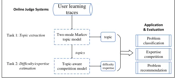
As shown in Fig.2, we focus on two tasks,topic detectionwhich automatically identifies the topics of a given problem anddifficulty/expertise level estimationwhich quantizes the difficulty level of a problem. The derived topic and difficulty/expertise information can be subsequently used in downstream OJ-related applications, e.g., problem recommendation or expert finding. Our proposed approaches have been evaluated on the programming OJ systems, but they are also applicable to any other OJ systems. Our contributions are summarized as follows:

• We present the first study to automatically learn topics and difficulty levels for problems on OJ systems where problems are simply organized by volumes.

• We quantitatively analyze the learning behaviors of users on OJ systems. We have identified two learning patterns, i.e., volume-oriented and topic-oriented learning. The observation is further explained and supported by the theories from educational psychology. Based on the above behavioral characteristics, we propose a two-mode hidden Markov topic model for learning topics of problems.

• We quantitatively analyze the distribution of difficulty levels over different topics. We have found that questions from different topics may have varying degrees of difficulty levels. Based on this finding, we develop a topic-specific expertise model for estimating problem difficulty levels and user expertise scores.

• Extensive experiments on three large online judge datasets have demonstrated the effec-tiveness of our approach in three different tasks, including skill topic extraction, expertise competition prediction and problem recommendation.

2 PROBLEM DEFINITION

Letu andqdenote a user and a problem respectively. Assume that there are a set of usersU and a set of problemsQ. Usually, the problems are organized in a volume setV. Each problem q belongs to a unique volumevq ∈ V. In an OJ system, a userucan submit her solution to a problemq. We call such an action anattempt. Each attempt happens at a timestamps and ends with a status labell. The timestamps are accurate to the second in the UNIX timing system, and the status label usually only has two possible values: Pass or Failed. Given a useru, we sort her Nu attempt records in an ascending order according to the timestamps, and obtain an orderedUser

Attempt Sequence(UAS):hq1,s1,l1i → hq2,s2,l2i →...→ hqi,si,lii →...→ hq_Nu,s_Nu,l_Nui, where we

haves1 <s2< ... <si < ... <sNu. With user attempt sequences, we can trace the attempts of a

user over time.

The attempt label reflects the individual competition result between a user and a problem. We further introduce a competition between two users on a problem. AnExpertise Competition Triplet

(ECT)hu,u0_{,qiconsists of two usersu,u}0_{and a problemq. Given a pair of users(u,u}0_{), we can} form an ECThu,u0_{,qiif there exists some intermediate problemqthat has been successfully solved} byubut not byu0_{. That is to say,ubeatsu}0_{on the problemq. To make the notations consistent,} we create a virtual useruqfor each problemq. Our final user setU is extended to the union set of the user set and problem set, i.e.,U0=U ∪ Q. In this way,hu,u_q,qican be used to represent the competition between a useruand a problemq.

With the above definitions, we are ready to define our two tasks, namelytopic extractionand

difficulty/expertise level estimation.

Definition 2.1. Topic Extraction.Topics here refer to the related components, skills and facts for structuring and organizing problems in a coherent way. The goal of topic extraction is to discover a set of skill topicsT in OJ systems, and each topiczis a multinomial distribution over the problems {ϕ_z,q}_q∈ Q.

For example, a sectional organization of C language programming can be listed as follows:

introduction,variables,loops and controls,arrays,structandpointersandIO. These sections can be considered as topics in a coarse granularity. It is worth noting that topic granularity is not pre-defined but automatically learned from data.

Definition 2.2. Difficulty/Expertise Level Estimation.The goal of difficulty/expertise level estimation is to infer the difficulty/expertise level of a problem or a user in OJ systems. Specially, given a useru(or problemq), it aims to estimate the expertise level ofuon each specific skill topic z, denoted bysu,z, which is a real scalar value in some predefined range. Similarly, we can usesq,z

to denote the difficulty level of problemqon topicz.

As discussed in [6,57], topics and difficulty levels are very important to be used to organize educational resources. Hence, our major focus of this work is to study how to learn them automati-cally based on users’ learning traces. To solve the above two tasks, we propose a topic modeling approach to learn topics and difficulty levels (Section4.1and4.2). Furthermore, we can utilize the identified topics and difficulty levels information to improve related applications in OJ systems such asproblem recommendation(Section4.3).

3 DATA COLLECTION AND ANALYSIS

We select three popular programming OJs for analysis and evaluation:

• Timus: Timus Online Judge is the largest Russian archive of programming problems with automatic judging system. Questions are mostly collected from contests held at the Ural Federal University, Ural Championships, Ural ACM ICPC Subregional Contests, and Petroza-vodsk Training Camps.

• POJ: Peking University Online Judge5is the most famous Chinese archive of programming problems. POJ has attracted the best programmers in China and even worldwide. • HDU: HDU6is hosted by Hangzhou Dianzi University from China. It consists of a large

number of problems for beginners, many of which are presented in Chinese.

On all the three platforms, problem resources are organized by volumes. OJ systems provide automatic assessment to users’ submitted solutions in a black-box test way. A problem consists of multiple test cases with the same input and output format. Only after a user’s submitted program-ming code passes all the test cases, the system would return the“Accepted"status, indicating the problem has been solved successfully. Programming OJ systems present in real-time a ranked list of users based on their number of accepted (a.k.a.solved) problems. The entire attempt record of a user is visible to all the other users. Such an open and competitive mechanism is one of the key successful factors for programming OJ systems [50].

5_{http://poj.org/}

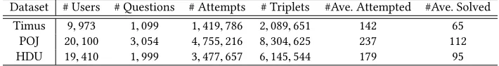
Table 1. Statistics of our datasets.

Dataset # Users # Questions # Attempts # Triplets #Ave. Attempted #Ave. Solved Timus 9,973 1,099 1,419,786 2,089,651 142 65

POJ 20,100 3,054 4,755,216 8,304,625 237 112 HDU 19,410 1,999 3,477,657 6,145,544 179 95

3.1 Construction of the Datasets

We crawl the data from the three OJ systems. At the time of crawling, the total numbers of registered users in Timus, POJ and HDU are 111,182, 715,002 and 460,322 respectively. Most of the tail users have made very few submissions, so we only keep the top users ranked by the number of accepted problems. To construct the user attempt sequence, we remove repeated attempts from a user on the same problem in a very short time period (i.e., 1 hour), and only keep the latest attempt with the Pass label. To construct the expertise competition triplets, we only use the final attempt result, i.e., onceuhas successfully solvedqregardless of how many times she has failed previously,uis considered to be able to beatq. The statistics of our datasets is presented in Table1.

Timus provides category (or topic) labels for some problems and difficulty scores for all problems. Out of 1,110 problems, 538 are tagged with one or multiple category labels from the category set {

Dynamic programming, Palindromes, Geometry, Tricky problem, Hardest problem, Data structures, Number theory, Graph theory problem for beginners, Game, Unusual problem, String algorithms}. For POJ and HDU datasets, there are no such labeled data. Nevertheless, we notice that some top performing users categorize the problems they have solved by topics in their blogs. We therefore use those category labels as the topic labels of problems. For problems with multiple category labels assigned by more than one user, we manually merge those labels. Finally, 458 out of 3,054 problems on POJ and 482 out of 1,999 problems on HDU have been annotated with a topic label (which was proposed by at least two users) using a similar category set from Timus. We do not annotate the difficulty levels for the problems on POJ and HDU, since they are not used explicitly as ground truth in our evaluations.

3.2 Basic Analysis and Observations

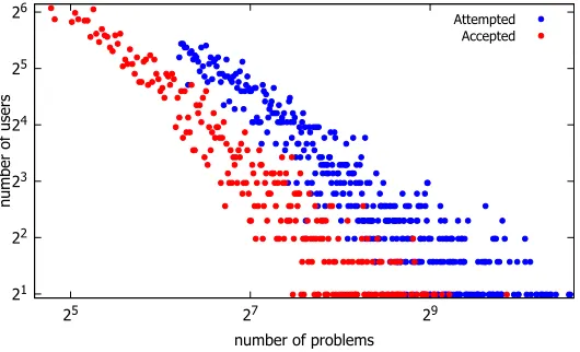
Given the datasets, we conduct some initial analysis on the Timus dataset. Our findings on the other two datasets are similar and are hence omitted here. First, we plot the distributions of the number of users with respective to their numbers of attempted or accepted problems in Fig.3. We can observe that both distributions show a clear power-law like shape, which indicates that only a small fraction of users have attempted or solved many problems.

We then conduct further analysis related to topics and difficulty levels and make the following observations.

Observation 1:A user is likely to make consecutive attempts on problems from the same volume.

21 22 23 24 25 26

25 ₂7 ₂9

number of users

number of problems

Attempted Accepted

Fig. 3. Distributions of usersw.r.t.the number of accepted or attempted problems on the Timus dataset in log-log scale. We have excluded users with few attempts for ease of data crawling.

Observation 2:A user is likely to make consecutive attempts on problems under the same topic.

Similar to the above analysis, we continue to study the effect of the topic information on users’ learning behavior. For each user, we sample thirty short windows consisting of five attempts (we remove consecutive repetitive submissions). Then we make pairwise comparisons between two labeled problems (problems without labels are ignored here) from a window and check whether they belong to the same topic category. We have found that about 41.4% problem pairs are indeed labeled with the same topic. The ratio is also significantly larger than the reference ratio 8.3%, which is estimated by_TT_×T andT(=12)is the total number of topic categories on Timus. Unlike the analysis inObs. 1, the estimated ratio here is only an approximation, since only half of the problems were annotated with the topic labels. Although the problems are organized by volumes without any topic information, the users still show a strong learning pattern by working on the same topic consecutively.

Observation 3:Questions from different topics may have varying degrees of difficulty levels.Here we analyze the characteristics of the distribution of difficulty levels for problems under different topics. We plot the distributions over 12 topic categories in Figure4. It can be observed that the distribution of difficulty scores highly depends on topics.

0 2000 4000 6000 8000 10000 12000 14000 16000

C01 C02 C03 C04 C05 C06 C07 C08 C09 C10 C11 C12

Di

ffi

cu

lty

Distribution of difficulty of questions from Timus grouped by different subjects

Fig. 4. The distribution of difficulty scores by topics on the Timus dataset. For ease of visualization, we use Cito index the categories. C01∼C12refer to Dynamic programming, Palindromes, Geometry, Tricky problem, Hardest problem, Data structures, Number theory, Graph theory problem for beginners, Game, Unusual problem, String algorithms respectively. A larger score indicates a higher difficulty level.

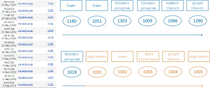
user with nickname ofmomohuanghas attempted 12 problems. It can be seen that the first seven attempts are topic-oriented, while the last five attempts are volume-oriented.Obs.1 and 2 also motivate us to develop a two-mode Markov topic model to characterize users’ learning behaviors for topic extraction (Section4.1).

1180 1051 1303 1009 1086 1280

Game Game dynamic

program

dynamic program

number theory

graph theory

1018 1001 1002 1003 1004 1005

dynamic

program beginners none

data structure

graph

theory beginners

As forObs.3, we have observed that the difficulty levels of problems from different topics are different and varying. We could utilize the topic information of problems for better characterizing difficulty levels of problems.Obs.3 thus motivates us to develop an approach to model problem difficulty and user expertise levels (Section4.2).

4 A TOPIC MODELING APPROACH FOR LEARNING TOPICS AND DIFFICULTY

LEVELS

In Section3.2, we have made some interesting observations about topics and difficulty levels. In this section, we study how to develop our solution for topic extraction and difficulty level estimation based on these findings. A key point is that the entire learning process should be unsupervised and rely on no or little labeled data, since it is the actual case for most of OJ systems. Hence, we adopt the topic modeling approach, which is able to generate meaningful soft clusters for “words", i.e., problems in our setting. Our approach can effectively extract skill topics, and further learn the topic-specific difficulty/expertise levels. In what follows, we start by studying how to learn topics in Section4.1and subsequently followed by the estimation of difficulty levels of problems in Section4.2. In Section4.3, we introduce some downstream applications that can be improved by our models. For clarity, we first present the notations used throughout the paper in Table2.

4.1 Topic Extraction using a Two-Mode Hidden Markov Topic Model

Based on our definition, a user attempt sequence presents the learning trace consisting of her attempts on problems in a given time span, which is essentially a behavior sequence of user actions. We would like to capture the relatedness reflected in user behavior sequences, and infer topic information from there. Specifically, we adopttopicsfrom topic modeling [5] to model the grouping or clustering of problems. As shown inObs.1 and 2, there are two different learning patterns to consider, either volume- or topic-oriented modes. To characterize both learning modes, we incorporate two kinds of topics in our model, namely volume topics and skill topics. Volume topics correspond to the volumes set up by OJ systems, while skill topics correspond to topics related to different skills. Since a problem attempt is likely to be influenced by both learning modes, we have to jointly characterize them in order to more accurately model the generative process for problems. We start to discuss how to model each type of relatedness separately, and then combine these two parts in a joint model.

4.1.1 Volume-Oriented Sequential Relatedness.As we can see inObs.1, a user is likely to make consecutive attempts on problems from the same volume. Such a behavioral pattern is similar to that of the click behavior [7] in the field of Information Retrieval. Since the problems are present to a user by volumes, once a user has attempted or solved a problem from a specific volume, the remaining problems from the same volume are more likely to attract the user’s attention than those from other volumes. To capture this kind of behavioral relatedness, we introduce a set of

volume topics. Formally, letϕV_v denote the topic model corresponding to the volumev, where the superscript ofV stands for “volume". The probability ofϕV_v,qdenotes the conditional probability of a problemqfrom a volume topicv. Different from standard topic models, which have non-zero Bayesian priors over all the problems, we make a constraint on volume topics: only the problems from the volumevcan be assigned with a non-zero probability byϕ_vV. Furthermore, each user uhas a preference distribution over the volume topics, modeled by a multinomial distribution θV

u. In order to generate a problem from a volume topic, we first draw a volume topic label, and

Table 2. Notations and explanations.

Notations Explanations

u a user

Nu number of attempts by useru

q a problem

qu the attempt sequence of useru

n an index variable to the attempts

v a volume or volume topic

z a skill topic

c binary continuity indicator

y binary mode indicator

KS _{number of skill topics}

KV _{number of volumes}

ϕS

k thek-th skill topic

ϕV

k thek-th volume topic

θS

u the preference distribution ofuover the skill topics

θV

u the preference distribution ofuover the volume topics

ρS

u the Bernoulli distribution over the continuation of skill topics

ρV

u the Bernoulli distribution over the continuation of volume topics xu,n the features related to then-th attempt from useru

ϵ the weight vector of the logistic classifier eu(q) the expertise score of useruwith the context ofq xq the topical probabilities related to queryq

bu the base expertise score of useru su topic-specific expertise vector of useru

w the importance vector of topics

µu,σu Gaussian parameters for useru α,β,ψ prior parameters of the topic models

current attempt depends on the topic label of the previous attempt. Formally, we assume that a user is associated with a Bernoulli distributionρVu. At then-th attempt, a user first draws a binary

indicator variablecu,n ∼Bern(ρV_u). Ifcu,n =0, we keep and reuse the volume topic label of the

previous problem, i.e.,vqu,n =vqu,n−1; otherwise, we draw a new topic label using the user-specific preference distributionθVu.

4.1.2 Topic-Oriented Sequential Relatedness.We continue to model the topic-oriented sequential relatedness inObs.2. Formally, letT denote a set of skill topics, each of which is a multinomial distribution over the problems, denoted byϕSz, and the probabilityϕSz,q, i.e.,Pr(q|z), indicates the

conditional probability that a problemqis generated from topicz. We use the superscript ofSto discriminate skill topics from volume topics. Furthermore, each useruhas a preference distribution over a set of skill topics, modeled by a multinomial distributionθuS, in whichθuS,z indicates the

Table 3. The different generation routes with the two-mode topic models. “follow" and “re-draw" refer to whether the previous topic assignment is reserved or newly sampled.

yu,n yu,n−1 cu,n zu,n vu,n remark

1 1 1 − v ∼Multi(θV_u) volume-mode, re-draw

1 1 0 − v_u,n−1 volume-mode, follow

1 0 1 − v ∼Multi(θV_u) volume-mode, re-draw

0 1 1 z∼Multi(θ_uS) − topic-mode, re-draw

0 0 1 z∼Multi(θ_uS) − topic-mode, re-draw

0 0 0 zu,n−1 − topic-mode, follow

n-th attempt, a user first draws a binary indicator variablecu,n ∼Bern(ρS_u). Ifcu,n =0, we keep and reuse the skill topic label of the previous problem, i.e.,zqu,n =zqu,n−1; otherwise, we draw a new topic label using the user-specific preference distributionθuS.

4.1.3 The Two-Mode Markov Topic Model.After describing the two kinds of learning patterns separately, we are ready to integrate them in a unified model. Our core idea is that a user has two optional learning modes to select, either volume-oriented or topic-oriented, indicating whether a user is likely to work on problems from the same volume or under the same skill topic. We use another hidden variableyto control the mode switch. The mode indicator variableyu,n is

drawn from a user-specific Bernoulli distribution, denoted byηu. The parameterηucharacterizes the tendency of useruto select over the two modes. With the incorporation ofy, we can code the different generation routes in Table3. Note that we use the same binary indicator variablec to model the Markovian relatedness for both kinds of topics. As we can see in Table3, we can control and select the corresponding mode using a certain combination ofyandc. Once these two variables are set, we can easily generate an attempted problem by a user. When determining the continuity variablec, we apply a hard constraint: onceyhas changed,chas to be re-drawn. Note that entries for the cases whereyu,n ,yu,n−1andcu,n =0 are invalid, since the topic variable has

to be re-drawn once the mode indicator has changed.

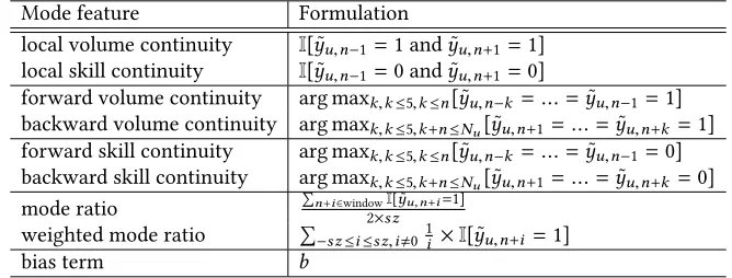
Table 4. The list of auxiliary features used in the logistic classifier for mode se-lection._I[·]is an indicator function which returns 1iff when the condition is true.

Mode feature Formulation

local volume continuity I[ ˜yu,n−1=1 and ˜yu,n+1=1]

local skill continuity I[ ˜yu,n−1=0 and ˜yu,n+1=0]

forward volume continuity arg maxk,k≤5,k≤n[ ˜yu,n−k =...=y˜u,n−1=1]

backward volume continuity arg maxk,k≤5,k+n≤Nu[ ˜yu,n+1=...=y˜u,n+k =1]

forward skill continuity arg maxk,k≤5,k≤n[ ˜yu,n−k =...=y˜u,n−1=0]

backward skill continuity arg maxk,k≤5,k+n≤N_u[ ˜yu,n+1=...=y˜u,n+k =0]

mode ratio Pn+i∈windowI[ ˜yu,n+i=1]

2×sz

weighted mode ratio P

−sz≤i≤sz,i,0

1

i ×I[ ˜yu,n+i =1]

U

ρV u

ρS u

cu,2

cu,1

ku,1 ku,2

qu,1

ε

cu,n

qu,2

θS u

θV u

KV

βV _βS

KS

φV _φS

ψV

ψS

αV

αS

...

ku,n

qu,n

...

...

...

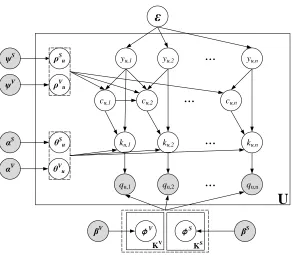
Fig. 6. The plate notation of the proposed model.

4.1.4 Enhancing the Mode Learning with Auxiliary Features.In the above, the mode preferenceηu

is drawn from a symmetric Beta prior. The learning ofηufully relies on the sequential characteristics of the the trace data. Here, we further propose to incorporate useful auxiliary features for deriving the prior knowledge in determining the mode. Our idea is inspired by the observation in Fig.5. Although it is difficult to identify the topic mode (since the topic itself is hidden), it is relatively easy to collect evidence that is useful to identify the volume mode. Intuitively, in a short window, if multiple attempted problems are from same volume and also have nearby problem IDs, it is probable to be in the volume mode. We compile a list of such auxiliary features, and derive a feature vectorxu,nfor then-th attempted problem by useru. We then train a binary logistic classifier to set the mode selection probability. The probability that selects the volume mode can be set below

Pr(yu,n =1|x_u,n,ϵ)= 1 1+exp(−ϵ>_·x

u,n), (1)

whereϵis the weight vector for the logistic classifier. Once we have obtained the above conditional probabilities, we can then generate the mode by usingηu as the prior. Unlikeηu, Pr(y=1|xu,n,ϵ)

is both user-specific and attempt-specific. Even for the same problem, when it appears in different sequential contexts, the mode selection probability will vary according to the actual context. For each attempt, we pre-compute a local volume mode indicator ˜yu,n. We set ˜yu,n to 1,iff (1) vu,n−1 =vu,n =vu,n+1and (2) the problem ID differences are smaller than a threshold of∆, i.e.,

|q_u,n −q_u,n−1| ≤ ∆and|qu,n −qu,n+1| ≤ ∆. We set∆to 20. ˜yu,n can be considered as a good

1. For each skill topick =1, ...,KS,

(1) draw a multinomial distributionϕ_kS∼Dir(βS); 2. For each volume topicv=1, ...,KV,

(1) draw a multinomial distributionϕV_v ∼Dir(βV), setϕV_v,q=0, ifvq ,v; 3. For each useru=1, ...,|U |,

(1) draw a multinomial distributionθ_uS∼Dir(αS); (2) draw a multinomial distributionθV_u ∼Dir(αV); (3) draw a Bernoulli distributionρV_u ∼Beta(ψV); (4) draw a Bernoulli distributionρS_u ∼Beta(ψS);

(5) For each problemqu,n(n=1, ...,Nu) in the attemp sequence byu, (i.) draw the mode variableyu,n ∼Pr(y|x_u,n,ϵ);

(ii.) drawcu,nby,

cu,n =

          

1 ifyu,n ,yu,n−1,

c∼Bern(ρV_u) ifyu,n =yu,n−1=1,

c∼Bern(ρSu) ifyu,n =yu,n−1=0.

(iii.) sample topicku,nby,

ku,n =

          

ku,n−1 ifcu,n =0,

v ∼Multi(θV_u) ifyu,n =1,cu,n =1,

z∼Multi(θ_uS) ifyu,n =0,cu,n =1. (iiii.) sample the problemqu,n by,

qu,n =

    

q∼Mul(ϕV_v) ifyu,n =1,ku,n =v,

q∼Mul(ϕ_zS) ifyu,n =0,ku,n =z.

Fig. 7. The generative process of the two-mode Markov topic model.

indicator ˜yu,n, we can derive a series of compositional features based on ˜yu,nfrom a short window

as summarized in Table4.

4.1.6 Inference and Parameter Learning.In our model, the parameters to learn are topics{ϕS_z} and{ϕV_z}, users’ preferences{θ_uS}and{θ_uV}, switch distributions{ρV_u}and{ρ_uS}, and the logistic weightsϵ. The hyper-parametersα,β,ψare set to small values empirically. We need to infer the values of hidden variables, i.e.,c,yandz.

LetΨdenote all the hyper-parameters. We first derive the joint likelihood of all the variables (both hidden and observed) conditional on the hyper-parameters. For clarity of derivation, we do not expand the probability ofPr(ϕS_z,ϕV_z,θ_uS,θ_uV,ρV_u,ρS_u,ϵ|Ψ). The joint likelihood is given below

Pr(k,y,c,q,ϕS

z,ϕVz,θuS,θuV,ρVu,ρuS,ϵ|Ψ)

=

| U |

Y

u=1

Nu

Y

n=1

Pr(yu,n|u,ϵ)Pr(c_u,n|ρ_u,y_u,n,y_u,n−1)Pr(ku,n|ku,n−1,yu,n,cu,n,θuS,θuV)

Pr(qu,n|yu,n,ku,n,ϕVku,n,ϕ

S ku,n)Pr(ϕ

S

z,ϕVz,θuS,θuV,ρVu,ρSu,ϵ|Ψ),

(2)

where we useku,nto denote either type of topics, and the rest factors can be expanded as follows

Pr(yu,n =1|x_u,n,ϵ) = 1

1+exp(−ϵ>_·x_u,n). (3)

Pr(cu,n|ρu,yu,n,yu,n−1) =

          

1 ifyu,n ,yu,n−1,

ρV

u ifyu,n =yu,n−1=1,

ρS

u ifyu,n =yu,n−1=0.

(4)

Pr(ku,n =k|k_u,n−1,yu,n,θuS,θVu) =

          

I[ku,n−1=k] ifcu,n=0,

θS

u,k ifyu,n =1,cu,n =1,

θV

u,k ifyu,n =0,cu,n =1.

(5)

Pr(qu,n=q|y_u,n,k_u,n,ϕV_k

u,n,ϕ

S

ku,n) =

     ϕS

z,q ifyu,n =0,ku,n=z,

ϕV

v,q ifyu,n =1,ku,n=v. (6)

Our objective is to jointly optimize the above likelihood given the hyper-parameters. Since it involves both observed and hidden variables, it is computationally infeasible to perform direct optimization. In this work, we develop a method to perform approximate inference following the standard parameter estimation method for HMMs. Our model captures two types of sequential relatedness, namely topic-oriented and volume-oriented, in a chain-like structure. The user attempt sequence essentially forms a Markov chain. The topic assignment of an attempt will depend on its preceding attempt. Specially, in our model, each hidden triplethc_u,n,y_u,n,k_u,nistands for the state of the current attempt, which consists of three hidden assignments. So, the total number of hidden states in our model is(2· |T |+2· |V |). For each skill or volume topic, we associate it with two unique states to indicate whether it follows the previous assignment or is re-drawn. Following the standard Expectation-Maximization algorithm, we use the E-step is to infer the values for hidden variables, and the M-step to optimize the parameters. We omit the derivation details, and present the update formulas for the E-step and M-step.

E(Cz,q) =

| U |

X

u=1

Nu

X

n=1

Pr(qu,n =q,ku,n =z,yu,n=0|q_u), (7)

E(Cv,q) =

| U |

X

u=1

Nu

X

n=1

Pr(qu,n =q,ku,n =v,yu,n =1|qu), (8)

E(Cu,z) = Nu

X

n=1

(

Pr(yu,n =0,yu,n−1=1,ku,n =z|qu), (9)

+Pr(yu,n =0,yu,n−1=0,cu,n =1,ku,n =z|qu)

)

, (10)

E(Cu,v) =

Nu

X

n=1

(

Pr(yu,n =1,yu,n−1=0,ku,n =v|q_u), (11)

+Pr(yu,n =1,yu,n−1=1,cu,n =1,ku,n =v|qu)

)

, (12)

E(Cu,n,i) = Pr(yu,n=1|qu), (13)

E(Cu,n,s) = Pr(yu,n=0|q_u), (14)

wherequ is the attempt sequence by excluding then-th attempt.

While for the M-step, we can perform the following update to optimize the parameters

ϕvV,q ∝ E(Cv,q)+βV −1, (15)

ϕS

z,q ∝ E(Cz,q)+βS−1, (16)

θuV,v ∝ E(Cu,v)+αV −1, (17)

θS

u,z ∝ E(Cu,z)+αS−1, (18)

ρS

u =

PNu

n=2Pr(yu,n=0,yu,n−1=0,cu,n =1|qu)+ψS

PNu

n=2Pr(yu,n =0,yu,n−1=0|qu)+2ψS

, (19)

ρV

u =

PNu

n=2Pr(yu,n=1,yu,n−1=1,cu,n =1|qu)+ψV

PNu

n=2Pr(yu,n =1,yu,n−1=1|qu)+2ψV

. (20)

As we also have logistic parameters involved in the model, we need to learn the logistic weights

ϵby maximizing the following objective function in the M-step.

ϵj+1₌

argmax ϵ

| U |

X

u=1

Nu

X

n=1

E(Cu,n,i)logPr(yu,n =1|x_u,n,ϵ)+E(C_u,n,s)logPr(yu,n =0|x_u,n,ϵ), (21)

which can be optimized by using a stochastic gradient descent method

∂J(ϵ)

∂ϵf (22)

=

| U |

X

u=1

Nu

X

n=1

xu,n,f · (

E(Cu,n,i)· exp(− P

fϵf ·x_u,n,f) 1+exp(−P

fϵf ·xu,n,f)

−E(C_u,n,s)· 1 1+exp(−P

fϵf ·xu,n,f) )

,

In order to avoid local minima as commonly encountered when using the EM algorithm, we train the model with multiple random initializations.

4.2 Difficulty and Expertise Level Estimation using a Competition Model with Topical

Contexts

In the above, we have studied how to learn topics using the two-mode Markov topic model. The proposed model is able to capture the sequential relatedness from two learning modes. Our final model outputs a set of skill topics (i.e.,{ϕS_z}), each of which groups problems with coherent skills under a specific topic. Now, we continue to study how to estimate user expertise and problem difficulty levels by introducing a novel competition model. Recall that we have created a virtual user for each problem (Section2), we thus do not need to discriminate between user expertise and problem difficulty unless otherwise specified. Our focus is to predict (1) whether a useruis qualified to solve a problemq; and (2) whether is a useruis more capable of solving a problemq than another useru0_.

4.2.1 The Bradley-Terry comparison model.The estimation for user expertise and problem difficulty levels has been widely studied in the past [13,21]. Most of existing studies assume that each user or problem is associated with a single expertise or difficulty score. Our base model is built on the classic Bradley-Terry model [47], which is the basis of many research works in pairwise comparison. In the Bradley-Terry model, each player’s strength is represented by a single real number, and the probability of playerubeating playeru0_{is modeled as}

Pr(ubeatsu0) = exp(eu) exp(eu)+exp(eu0)

, (23)

= 1

1+exp(−(e_u−e_u0)) ,

= S(eu,eu0),

whereeu andeu0are the expertise scores of useruandu0respectively. The Bradley-Terry model

essentially adopts the sigmoid function which takes the difference between the strengths of the two players. The actual “competition" case can be very complex, and a single expertise score has a relatively weak capability to measure the expertise level of a user or a problem in varying contexts. Hence, we consider incorporating the contextual information for two-player comparison into the Bradley-Terry model. Given the ECThu,u0,qi, a problem has to be specified as the context of a competition, which is defined below

Pr(ubeatsu0|q) = exp(e

(q)

u )

exp(eu(q))+exp(eu(q0))

, (24)

= 1

1+exp−(e_u(q)−e_u(q0)) ,

= S(eu(q),eu(q0)),

whereeu(q)is the expertise score thatuattempts onq. In other words,eu(q)is the expertise score of

4.2.2 Expertise Modeling with Topical Contexts.In order to defineeu(q), we have to consider two

points: (1) how to represent the contextual information from problemq; and (2) how to define the context-aware expertise scoreeu(q). First, we extract the skill topic information related to a problem

and define the context as the distribution over the skill topics. Formally, for each problemq, we can obtain its conditional probabilities in all the skill topics, i.e.,{ϕS_k,q}_k. Note that these conditional probabilities{ϕS_k,q}_kfor problemqdo not sum to 1. For simplification of notations, we usexqto denote theKS-dimensional vector consisting of the probability set{ϕS_k,q}_k for problemq. In this way, the contexts from all the problems can be represented in a unified way. After introducing topical contexts, we can further define the topic-aware expertise. Formally, we assume that a user uis associated with a base expertise scorebu, which is static and fixed. In addition, letsu ∈RKS

denote a topic-specific expertise vector for useru, where each entrysu,kdenotes the expertise level

of useruon thek-th topic. With the above definitions, we can define the expertise score that user uattempts to solve problemqas follows

eu(q) = w>·x_qs_u | {z }

problem-specific expertise

+ bu

|{z}

base expertise

, (25)

wherew ∈ _RKS is a weight vector which measures the global importance for different topics,

xq ∈ RKS is a contextual vector with topical information for problemq, and “” denote the

element-wise product for vectors. By incorporating the problem as context, the topical vectorxq

weights the topic-specific expertise vectorsu in different topic dimensions. In this way,eu(q) is

decomposed into two parts, namely base expertise score and problem-specific expertise score. We further put prior on the model parameters. The base score is drawn from a user-specific Gaussian distribution, i.e.,

bu ∼ N(µu,σu), (26)

whereµu andσu are the prior parameters of a Gaussian distribution, which are user-specific. Similarly, the topic-specific expertise vector can be drawn as follows

su ∼ N(µu,Σu), (27)

whereµu =[µu, ...,µu]>_{is aK}S_{-dimensional vector ofµ}

1. Draw a global topic importance vectorw ∼ N(0,I); 2. For each useru=1, ...,|U |

(1) setµu andσuusing TrueSkill;

(2) draw the base expertise scorebu ∼ N(µ_u,σ_u);

(3) draw the topic-specific expertise vectorsu ∼ N(µ_u,σ_uI); (4) derive the context-aware expertise scoreeu(q)using Eq.25;

3. For each problemq=1, ...,|Q |,

(1) derivexq using the topic model in Section4.1; 4. For each ECThu,u0,qiin the dataset,

i. draw the competition result using Eq.24.

Fig. 8. The description of the topic-based competition model.

4.2.3 Optimization.After definingeu(q), we can plug Eq.25into Eq.24and derive the probability

for a ECThu,u0,qi, which indicates thatubeatsu0on the problemq. In other words,usuccessfully solvedqbutu0failed in solvingq. We present the overall objective function to learn the expertise score using the training ECT setDas below

L(G)= X

hu,u0_{,qi∈ D}

log Pr(ubeatsu0|q,Φ)+λlog Pr(Φ), (28)

where the loss function is essentially a Bayesian decomposition in a log form, andΦdenote all the related parameter, includingw, base scores{b_u}and topic-specific expertise vector{s_u}.

Note that we have created a virtual user for each problem. We treat the related expertise score from each virtual user as the difficulty level of its corresponding problem. To generate the training ECT set{hu,u0_{,qi}, we need to consider two types of comparisons: (1) a userv.s.a problem, and} (2) a userv.s.another user. The first type is achieved by mapping problems to virtual users, while the second type can be constructed by selecting intermediate problems. Once the triplets have been generated, we can adopt the standard Stochastic Gradient Descent approach for parameter optimization. At each time step, we sample a mini batch of 128 ECTs and then update the parameters involved in these ECTs.

4.3 Applications of the Proposed Approaches to Online Judge Systems

In this section, we discuss how to apply the proposed approaches to improve OJ systems.

4.3.1 Topic Extraction and Problem Classification.The learned skill topics (e.g.,dynamic

pro-gramming,backtracking, etc.) using our proposed two-mode Markov topic model can be helpful to organize problems in a topical way. Here, we consider a practical application, i.e., how to perform problem classification based on the learned skill topics. Given a set of predefined categoriesA, we would like to classify a problemqusing very little labeled data{(q0_,a

q0)|a_q0 ∈ A}. We classify a

aq = argmax

a∈ A

Pr(q|a), (29)

= argmax

a∈ A

Y

aq0=a

Pr(q|q0),

= argmax

a∈ A

Y

aq0=a X

z∈ T

Pr(q|z)×Pr(z|q0),

∝ argmax

a∈ A

Y

aq0=a X

z∈ T

Pr(q|z)×Pr(q0|z)×Pr(z),

wherezis a skill topic, and the involved three factors Pr(q|z),Pr(q0_{|z),Pr(z)can be directly obtained} using our model. We assume that the number of labeled problems is the same for each category.

4.3.2 Expertise Level Estimation and Competition Prediction.Our expertise model can generate expertise scores for both users and problems. Since we create a virtual user for each problem, problem difficulty and user expertise can be measured in the same scale. Following Eq.24, we can predict the outcome of (1) an attempt of a user on a problem; or (2) a competition between two users on a problem.

4.3.3 Problem Recommendation.By combining the above two aspects, the third application aims to recommend problems to a user by considering both aspects oftopical interestsandexpertise levels. Intuitively, a user has a topical preference over the problems, and would attempt the problems that have matched her topical interests. Also, a user cannot solve problems beyond her expertise level. We can therefore make recommendations of problems to users by combining these two factors.

Specially, we consider two scenarios for recommendation. The first scenario is overall recom-mendation, which aims to generate a list of time-insensitive recommendations, while the second scenario is the next-basket recommendation, which predicts the problems that a user is going to attempt next. Formally, the overall recommendation task can be casted as a similarity evaluation problem between a useruandqas follows

scoreover all(u,q) = (

X

v

ϕV

v,q·θVu,v·ηu+ X

z

ϕS

z,q·θuS,z·(1−ηu) )

| {z }

Interst

×Pr(ubeatsuq|q) | {z }

Expertise

, (30)

where Pr(ubeatsuq|q)is defined in Eq.24. Our scoring function considers both topical interests and expertise scores. For topical interest, we further calculate two preference scores for skill and volume topics respectively.

scorenext(u,q) (31)

= Pr(qu,n =q|u,q_u,1,· · ·,q_u,n−1,Φ)

| {z }

Interst

×Pr(ubeatsuq|q) | {z }

Expertise

= Pr(yu,n|u,ϵ)

×Pr(cu,n|ρ_u,y_u,n,y_u,n−1)

×

K X

z=1

Pr(ku,n =z|k_u,n−1,yu,n,cu,n,θuS,θuV)

×Pr(qu,n|y_u,n,k_u,n,ϕV_k

u,n,ϕ

S ku,n)

×Pr(ubeatsuq|q),

where the first four terms are defined in Eq.3to Eq.6respectively, and Pr(ubeatsuq|q)is defined in Eq.24.

Different from conventional recommendation algorithms, we incorporate expertise into consid-eration for recommendation. We decrease the score of a candidate problem which matches the interests of a user well but exceeds her expertise level. The learned topic information is mainly used for interest-driven recommendation, while the learned expertise/difficulty information is mainly used for expertise-based recommendation. The final recommendation is a balanced trade-off between these two factors.

5 EXPERIMENTS

In this section, we conduct experiments on the three datasets presented in Table1to evaluate our proposed models on the three application scenarios mentioned in Section4.3, namely, skill topic extraction, expertise competition prediction and problem recommendation.

5.1 Skill Topic Extraction

Automatic learning of skill topics for problems is extremely important for OJ systems since the learned topics can be used to group problems which makes it more easier for users to search for problems under certain topics.

5.1.1 Experimental setup.Recall that for each of the three datasets, we have the topic or category labels for a fraction of problems. Hence, our experiments are evaluated only using the partial set of labeled problems. We evaluate our approach in the following aspects, namely, topic similarity, topic purity and problem classification.

• Topic similarity: Given a problemq, we can obtain a vector{ϕ_z,q}_z∈ T consisting of its probabilities generated by each topic, where each entryϕz,qis the probability of problem qgenerated by topicz. The intuition is that if two problems are from the same category, then their topic-probability vectors should be also similar. Based on this idea, given two categories, we compute the average similarity between the learned topic-probability vectors for the problems in the two categories. Formally, letC₁andC₂denote two labeled problem sets, each of which corresponds to a category. We compute the pairwise similarities between two categories as follows

sim(C₁,C₂)= 1 |C₁| ∗ |C₂|

X

q∈ C₁

X

q0_{∈ C}

2

P

z∈ T ϕz,q·ϕz,q0 kϕ_·,q k₂· kϕ_·,q0 k₂

where we use the cosine similarity to measure the similarity between two topic-probability vectors.

• Topic Purity: Topic models can be considered as a soft clustering of items. Hence, we measure the quality of the generated skill topics usingpurity, a commonly used metric for clustering evaluation. Given a topic, we take the top ten problems to form a cluster. Then we compute the purity score for a set of topics as follows

Purity(T)= 1 |T |

X

z∈ T

Na(zmax)

P a0N_a(z₀)

, (33)

whereNa(z)denote the number of problems with the category labelaandamax is the most common category label in topicz.

• Problem classification: The eventual goal of learning skill topics is to classify problems into categories. We follow the derivations in Section 4.3 to classify a problems as follows

aq ∝arg max

a∈ A

Y

aq0=a X

z∈ T

Pr(q|z)×Pr(q0|z)×Pr(z), (34)

where we only use five labeled problems for each category. Since it is a multi-classification task, we use the F1 and accuracy as the evaluation metrics.

5.1.2 Methods to Compare.We compare our model with three topic models and a Hidden Markov Model.

• LDA: We use the Latent Dirichlet Allocation [5] to generate skill topics. We first combine all the attempted problems by a user as a document, then run the standard LDA model using GibbsLDA++ [41]. LDA does not consider the order of word tokens, and it cannot discriminate between skill topics and volume topics. We apply the default settings in [22], i.e.,α=50/K,β=0.01.

• LDA_text: Instead of using problems as word tokens, we directly crawl the textual problem descriptions from OJ websites. Then we remove the stopwords and run the standard topic extraction using the LDA model. Note that in this method, we cannot learn problem topics but instead word topics. Hence, we only use LDAtext in the evaluation of problem classification. The hyper-parameters are set asα=50/K,β=0.01.

• HTMM: It is the Hidden Markov Topic Model [24], in which the order of tokens has been characterized based on the first-order Markovian property. In our setting here, the attempted problem sequence from a user is considered as a document. The hyper-parameters are set asα=1+50/K,η =1.01.

• HMM: It is the standard first-order Hidden Markov Model, which is used to characterize the attempted sequences. For fairness, we implement the HMM model using Gibbs sampling, where the state hidden variables can be considered as problem topics.

• Our model: It is our proposed model in Eq.29. We only use the learned skill topics for evaluation. The hyper-parameters are set as follows:αV =αS =1+50/K,βV =βS = 1.01,ψ=0.01.

We set the number of topics to 40 for all the compared methods based on a validation set of 10% training data.

while the other three methods have even distributions for category similarities. The results indicate that our generated skill topics are very effective to discriminate problems from different categories. We also find hat it is not easy to learn clear skill topics using traditional models like LDA and HMM. One main reason is that the generation of attempt sequences is a mixture of two learning modes. while the baselines can only consider one of the two modes.

c1 c2 c3 c4 c5 c6 c7 c8 c9 c10 c1 c2 c3 c4 c5 c6 c7 c8 c9 c10 Similarity

(a) Our model

c1 c2 c3 c4 c5 c6 c7 c8 c9 c10 c1 c2 c3 c4 c5 c6 c7 c8 c9 c10 Similarity

(b)HT M M

c1 c2 c3 c4 c5 c6 c7 c8 c9 c10 c1 c2 c3 c4 c5 c6 c7 c8 c9 c10 Similarity

(c)H M M

c1 c2 c3 c4 c5 c6 c7 c8 c9 c10 c1 c2 c3 c4 c5 c6 c7 c8 c9 c10 Similarity (d)LDA

Fig. 9. Heatmaps for pairwise category similarity measured by different topic models on the Timus dataset.

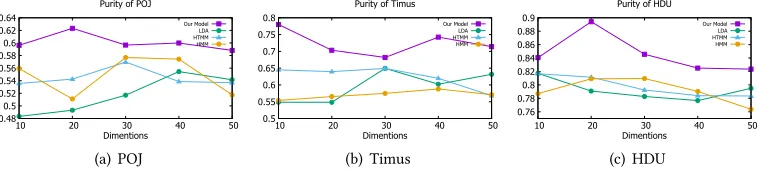
Next, we present the purity scores of different methods on the three datasets in Figure10. We vary the number of topics (or states in HMM) from 10 to 50 with a step of 10. It can be observed that our model is consistently better than the baselines in all the cases. For our model, a topic number of 20 gives best performance on the datasets of POJ and HDU, while a topic number of 10 gives best performance on the dataset of Timus. The main reason is that Timus has fewer problems than the other two OJ websites.

0.48 0.5 0.52 0.54 0.56 0.58 0.6 0.62 0.64

10 20 30 40 50

Dimentions Purity of POJ

Our Model LDA HTMM HMM (a) POJ 0.5 0.55 0.6 0.65 0.7 0.75 0.8

10 20 30 40 50

Dimentions Purity of Timus

Our Model LDA HTMM HMM (b) Timus 0.76 0.78 0.8 0.82 0.84 0.86 0.88 0.9

10 20 30 40 50 Dimentions

Purity of HDU

Our Model LDA HTMM HMM

(c) HDU

Fig. 10. Purity scores of different methods on three datasets.

We finally present the results of problem classification in Table5. We can make the following observations. First, the text-based LDAtextmodel is much worse than the problem-based LDA model, which indicates that the textual content is less useful for inferring the problem topics. Our result is consistent with the finding in [50], where it has shown that often times the problem statements are obscure for determining the topic information. Overall, the baseline HTMM performs the best among all the baselines, since it considers the sequential relatedness. Our model significantly improves over all the baselines with a large margin, which demonstrates the effectiveness of our model on problem classification.

Table 5. Performance comparison for problem classification on three datasets.

Methods PO J Timus HDU

F1 Accuracy F1 Accuracy F1 Accuracy LDA 0.659 0.713 0.464 0.49 0.564 0.596 LDAtext 0.382 0.413 0.341 0.392 0.387 0.396 HMM 0.605 0.647 0.568 0.596 0.546 0.592 HTMM 0.627 0.667 0.473 0.493 0.561 0.613 Our model 0.751 0.817 0.644 0.707 0.724 0.788

model on the Timus dataset in Table6. It is clear to see that the weights of volume-related features are positive while the weights of skill-related features are negative, which confirms to our intuition.

Table 6. Effect analysis of the weights for different features.I[·]is an indicator

function which returns 1iff when the condition is true.

Mode Feature Formulations Weight

local volume continuity I[ ˜yu,n−1=1 and ˜yu,n+1=1] 1.243

local skill continuity I[ ˜yu,n−1=0 and ˜yu,n+1=0] -3.186

forward volume continuity arg maxk,k≤5,k≤n[ ˜yu,n−k=...=y˜u,n−1=1] 1.261

backward volume continuity arg maxk,k≤5,k+n≤Nu[ ˜yu,n+1=...=y˜u,n+k =1] 1.261

forward skill continuity arg maxk,k≤5,k≤n[ ˜yu,n−k=...=y˜u,n−1=0] -0.201

backward skill continuity arg maxk,k≤5,k+n≤Nu[ ˜yu,n+1=...=y˜u,n+k =0] -0.775

mode ratio Pn+i∈windowI[ ˜yu,n+i=1]

2×sz 0.02

weighted mode ratio P

−a≤i≤sz,i,0 1i ×I[ ˜yu,n+i =1] 0.21

bias term b 1.519

Summary.Our model can effectively discriminate between the two learning modes, and generate clear skill topics. The learned skill topics enhance the within-category similarity and reduce the cross-category similarity. These topics have a higher purity score than the baselines. Moreover, they are helpful to improve the performance of problem classification.

5.2 Evaluation on Expertise Competition Prediction

Problem difficulty and user expertise estimation has been a hot research topic in educational data mining [11,42,64]. It is particularly useful to help schedule the curriculum and practice for students. In this part, we examine the performance of the proposed model on user expertise estimation.

5.2.1 Experimental Setup.In our task, it is infeasible to assign an absolute score to measure the difficulty level of a problem or the expertise of a user. Following the idea in ranking-based competition systems [28], we propose to use the competition based comparisons for evaluating the performance of various methods. Specially, we consider two kinds of competition scenarios, i.e., a userv.s.a problem and a userv.s.another user.

Table 7. Statistics of the three competition types on three datasets.

Datasets #UQ-AC # UQ-NAC # UUQ Timus 1,004,817 118,396 966,438

POJ 2,897,504 193,960 5,213,181 HDU 2,473,997 121,157 3,550,390

programming while another may be good at graph algorithms. Hence, it would be sensible to include a problem as the context. In this case, we essentially predict the outcome for the competition triplehu,u0,qi, i.e., whether useruis more capable than useru0for problemq. To generate such labeled triplets, we start by selecting a difficult problem, e.g., the problems with fewer than 500 accepted solutions. Given a selected problem, we further select a user pair, in which a user has solved this problem while the other user has failed in this problem. We denote the third competition type byUU Q. In this way, we can generate a large amount of labeled ECTs. We combine the labeled competitions for different types of competition scenarios and form a final evaluation set. We present the statistics of the thee competition types in Table7.

Since our datasets are imbalanced as there are moreU Q−AC competitions thanU Q−NAC competitions, we perform oversampling to duplicateU Q−NACcompetitions by five times. We then randomly split the labeled competitions with a ratio of 4:1 into training and test sets. For the training set, we take 10% to form the development set for optimizing model parameters. In our experiments, accuracy is used as the evaluation metrics, which is defined as follows:

ACC= #correctly_predicted_competitions

#all_competitions . (35)

5.2.2 Methods to Compare.The methods to be evaluated in our data are listed below:

• TrueSkill: The TrueSkill ranking system [28] is a skill based ranking system for Xbox Live developed at Microsoft Research. For each player, it characterizes her average skill and the degree of uncertainty in the player’s skill. We use the open source implementation from http://trueskill.org.

• Bradley-Terry: In the Bradley-Terry model, each playeru’s strength is represented by a single real numbereu, and the probability of playerubeating playeru0is modeled as

Pr(ubeatsu0) = 1

1+exp(−(e_u−e_u0))

. (36)

• PageRank: We follow [33] to build a competition graph consisting of users and problems as vertices. Then we run the standard PageRank algorithm on the competition graph. The final competition results are derived by comparing the PageRank scores.

• Blade-chest: Unlike standard preference-learning models that represent the properties of each item/player as a single number, the blade-chest method [8] infers a multi-dimensional representation for the different aspects of each item/player’s strength. We use the open-source implementation fromhttps://github.com/csinpi/blade_chest.

• AC rank: We simply rank users by their number of solved problems. Note the AC rank method can only predict the competition result between two users.

incorporate a base expertise in the proposed model. In addition, we consider two variants by removing the skill-specific expertise or base expertise, denoted byour model¬skill and our model¬baserespectively. We set the number of topicsKto 40.

It is worth noting that all the baselines cannot utilize the problem information in theUU Q com-petitions, since they can only characterize pairwise user expertise comparison without modelling problem context.

5.2.3 Results and Analysis.We report the performance of competitions in Table8. We can make the following observations.

• TrueSkill performs very well for the competition typeU Q−AC, but poorly forU Q−NAC. One main reason we have found is that TrueSkill tends to assign a higher expertise score to a user than a problem in the user-problem competition, since the majority of the attempted problems are essentially solved by users (See Table7). Although oversampling can alleviate this problem to some extent, TrueSkill is still sensitive to data imbalance.

• Compared with TrueSkill, Bradley-Terry and PageRank performs worse onU Q−ACbut better for the other two types. We have empirically found that Bradley-Terry and PageRank seem to be more robust to deal with imbalanced training data.

• The simple baseline AC rank works well for predictingUU Qcompetitions. The AC rank method is effective to discriminate between a skilled user and a new user. And ourUU Q competitions are created by first selecting difficult problems, which tends to generate more comparisons between users with different expertise levels.

• Blade-chest performs the best among all the baselines. It uses a multi-dimensional rep-resentation to characterize a player’s skill in multiple latent dimensions, which tends to represent users’ expertise more accurately.

• Our model is consistently better than all the baselines in all three competition types. The improvement over TrueSkill onU Q −AC is relatively small, but the improvement on the other two types is significant. We also report the performance from the variants by removing skill-specific or base expertise. As we can see, the incorporation of skill-specific expertise is the key to yield the major improvement.

Table 8. Performance comparison for expertise competition prediction on three datasets.

Methods PO J Timus HDU

UQ-AC UQ-NAC UUQ UQ-AC UQ-NAC UUQ UQ-AC UQ-NAC UUQ TrueSkill 0.922 0.645 0.831 0.942 0.635 0.826 0.945 0.689 0.828 Bradley-Terry 0.899 0.711 0.844 0.909 0.823 0.832 0.922 0.803 0.833 PageRank 0.901 0.793 0.834 0.912 0.831 0.855 0.902 0.815 0.831 Blade-chest 0.885 0.824 0.875 0.858 0.844 0.866 0.889 0.814 0.863

AC rank — — 0.853 — — 0.857 — — 0.846

our model¬base 0.924 0.851 0.870 0.942 0.872 0.888 0.939 0.876 0.881 our model¬skill 0.918 0.847 0.865 0.923 0.865 0.887 0.932 0.865 0.878 our model 0.929 0.868 0.884 0.944 0.874 0.897 0.943 0.881 0.886

5.3 Evaluation on Problem Recommendation

5.3.1 Experimental Setup.To make our evaluation more practical, we consider two recommen-dation scenarios. The first one is overall recommenrecommen-dation, which aims to recommend a list of problems based on the problems already attempted or solved by a user. The second one is next-basket recommendation for predicting the problems that a user is going to attempt in the next time period.

For overall recommendation, we randomly split the attempted or solved problems by a user with a ratio of 4:1 into training and test data. Similar to Information Retrieval, we usePrecision@kand Recall@k as the evaluation metrics.

For next-basket recommendation, we hold out the last ten attempted or solved problems by a user. Then we predict the held-out problems for a user in a sequential manner. In each time period, we assume that all the previous problems have already been observed, and we predict what the next problem is going to be for a user. Following [60], we adopthit@kas the evaluation metrics, which calculates the ratio of the correct predictions in the top ten recommendations for all the users.

For both tasks, we setk to 10. Specifically, for both recommendation scenarios, we can also consider either the attempted problems or the solved problems as the ground truth. The attempted problems reflect users’ interest, while the solved problems reflect both interest and expertise for users. We learn the models on the training data and examine its performance on the test data. We take 10% users from the training data as the development set to optimize model parameters.

5.3.2 Methods to Compare.We first present the methods to compare for overall recommendation.

• UserKNN: It is a classic collaborative filtering algorithm, which make the recommendations based on the top similar neighbors. We apply the Jarccard coefficient to find the most similar neighbors for a user based on her historical data. The number of similar neighbors is set to 50.

• PMF: It is the commonly used Probabilistic Matrix Factorization [37] model. We run the standard implementation of PMF on user-item interaction matrix. The number of latent factors is set to 40.

• BPR: It is the Bayesian Personalized Ranking model [48], which proposes a generic optimiza-tion criterion for personalized ranking that is the maximum posterior estimator derived from a Bayesian analysis. The number of latent dimensions is set to 40. BPR is a widely used baseline for recommendation with implicit feedback.

• NCF: It is the Neural Collaborative Filtering model [27], which utilizes deep learning techniques to enhance the modeling of user-item interactions. We follow the optimal setting tuned by [27] with three hidden layers. We also pretrain the NCF model as suggested in [27], which is important to improve its performance.

• Our model: It is our proposed model, which ranks the problems according to Eq.30. We also consider two variants of our model, which either removes interest modeling or expertise modeling. We denote the two variants byour model¬intandour model¬exp. The number of topics is set to 40.

Next, we present the methods to compare for next-basket recommendation.

• TOP: It is the frequency based recommendation method as mentioned before.

• MC: It is the frequency based Markov Chain model, which estimates the transition proba-bility between two problems using the maximum likelihood estimation method.