Micro Net : a unified model for segmentation of various objects in microscopy images

warwick.ac.uk/lib-publications

Persistent WRAP URL:

http://wrap.warwick.ac.uk/112011

How to cite:

Please refer to published version for the most recent bibliographic citation information.

If a published version is known of, the repository item page linked to above, will contain

details on accessing it.

Copyright and reuse:

The Warwick Research Archive Portal (WRAP) makes this work by researchers of the

University of Warwick available open access under the following conditions.

© 2018 Elsevier. Licensed under the Creative Commons

Attribution-NonCommercial-NoDerivatives 4.0 International

http://creativecommons.org/licenses/by-nc-nd/4.0/.

Publisher’s statement:

Please refer to the repository item page, publisher’s statement section, for further

information.

Micro-Net: A unified model for segmentation of various objects in

microscopy images

Shan E Ahmed Raza, Linda Cheung, Muhammad Shaban,

Simon Graham, David Epstein, Stella Pelengaris, Michael Khan,

Nasir M. Rajpoot

PII:

S1361-8415(18)30062-8

DOI:

https://doi.org/10.1016/j.media.2018.12.003

Reference:

MEDIMA 1438

To appear in:

Medical Image Analysis

Received date:

6 March 2018

Revised date:

13 December 2018

Accepted date:

14 December 2018

Please cite this article as: Shan E Ahmed Raza, Linda Cheung, Muhammad Shaban, Simon Graham,

David Epstein, Stella Pelengaris, Michael Khan, Nasir M. Rajpoot, Micro-Net: A unified model for

segmentation of various objects in microscopy images,

Medical Image Analysis

(2018), doi:

https://doi.org/10.1016/j.media.2018.12.003

ACCEPTED MANUSCRIPT

• A unified deep learning framework for segmentation of objects (cell nuclei, cells, and multi-cellular objects such as glandular structures) in two main

types of microscopy images: fluorescence and histology.

• The proposed Micro-Net is aimed at better object localization in the face of varying intensities and is robust to noise.

• Detailed experimentation & comparative evaluation on publicly available data sets and a new image dataset that is made public with this paper.

ACCEPTED MANUSCRIPT

Micro-Net: A unified model for segmentation of various

objects in microscopy images

Shan E Ahmed Razaa,b,∗_{, Linda Cheung}c_{, Muhammad Shaban}b_{, Simon}

Grahamb_{, David Epstein}d_{, Stella Pelengaris}c_{, Michael Khan}c_{, Nasir M.}

Rajpootb,e,f,∗

a_{Division of Molecular Pathology, The Institute of Cancer Research, UK.} b_{Department of Computer Science, University of Warwick, UK.}

c_{School of Life Sciences, University of Warwick, UK.} d_{Department of Mathematics, University of Warwick, UK.}

e_{Department of Pathology, University Hospitals Coventry and Warwickshire, UK.} f_{The Alan Turing Institute, London, UK.}

Abstract

Object segmentation and structure localization are important steps in

auto-mated image analysis pipelines for microscopy images. We present a

convolu-tion neural network (CNN) based deep learning architecture for segmentaconvolu-tion

of objects in microscopy images. The proposed network can be used to segment

cells, nuclei and glands in fluorescence microscopy and histology images after

slight tuning of input parameters. The network trains at multiple resolutions

of the input image, connects the intermediate layers for better localization and

context and generates the output using multi-resolution deconvolution filters.

The extra convolutional layers which bypass the max-pooling operation allow

the network to train for variable input intensities and object size and make it

robust to noisy data. We compare our results on publicly available data sets and

show that the proposed network outperforms recent deep learning algorithms.

Keywords: Cell segmentation, nuclear segmentation, gland segmentation,

convolution neural networks, microscopy image analysis, digital pathology

∗_{Corresponding author}

Email addresses: [email protected](Shan E Ahmed Raza),

ACCEPTED MANUSCRIPT

In automated microscopic image analysis pipelines, segmentation of key

structures such as tumours, glands and cells is an important step (Awan et al.

(2017); Yuan et al. (2012); Qaiser et al. (2017)). Recent advances in deep

learn-ing have helped to achieve accurate segmentation of these structures. A major

5

strength of deep learning is that the same network architecture can be used to

segment various structures across different modalities by retraining and slight

tuning of the input parameters (Shelhamer et al. (2017); Ronneberger et al.

(2015)).

In this paper, we propose a CNN with additional layers in the downsampling

10

path, bypassing the max-pooling operation in order to learn the parameters for

segmentation ignored during the max-pooling operation. By doing so, we retain

contextual information, make the network interpret the output at multiple

res-olutions and train the model at multiple input image resres-olutions in the

down-sampling path to learn the model parameters for variable cell/nucleus/gland

15

sizes and shapes in the presence of variable intensities and texture. There are

two main features of the proposed architecture: (a) it learns image features at

multiple input resolutions for better understanding of tissue components and

(b) it bypasses the max-pooling operation through extra layers to retain

infor-mation from weak features may be missed during max-pooling. This makes the

20

network robust to noise and helps to learn the context at multiple resolutions.

Figure 1 & 2 demonstrate the impact of these design changes. In Figure 1, solid

lines represent training accuracy/loss for Micro-Net and Micro-Net–_{, whereas}

dashed lines representvalidation accuracy/loss for Micro-Net and Micro-Net–

during training. Accuracy is defined in terms of pixel-wise agreement with the

25

ground truth and loss is defined in Section 3.6. In Micro-Net–_{, we removed}

the multi-resolution input and the bypass layers while keeping the rest of the

architecture the same. The improved accuracy and loss values demonstrate the

importance of the proposed design changes. To emphasise this further, Figure

2(a) shows an H & E image where nuclei are outlined with green boundaries by

ACCEPTED MANUSCRIPT

and Figure 2(c) the result of the proposed approach. It can be observed that

U-Net failed to learn the features due to the presence of a dark cytoplasmic

region and segmented most of the cellular region instead of just the nucleus,

whereas the proposed approach learned the context at multiple resolutions and

35

successfully located the nuclei despite high levels of noise. We discuss this in

detail in Section 4.

0 5 10 15 20

Epoch

0.68 0.7 0.72 0.74 0.76 0.78 0.8 0.82

0.84 Accuracy

Micro-Net: Training Accuracy Micro-Net: Validation Accuracy Micro-Net : Training Accuracy Micro-Net : Validation Accuracy

0 5 10 15 20

Epoch

1 1.5 2 2.5 3 3.5

4 106 Loss

Micro-Net: Training Loss Micro-Net: Validation Loss Micro-Net : Training Loss Micro-Net : Validation Loss

Figure 1: Solid lines represent training accuracy/loss for Micro-Net and Micro-Net– _while

the dashed lines represent validation accuracy/loss calculated for 25 epochs on fluorescence imaging data for cell segmentation. Micro-Net– _{was obtained by removing multi-resolution}

input and the bypass layers from Micro-Net architecture. The accuracy and loss curves clearly

show the importance of the multi-resolution input and bypass layers.

This paper is an extension of our previous work on cell (Raza et al. (2017a))1

and gland segmentation (Raza et al. (2017b)) with the following novel

contri-butions:

40

1_{We will publish our fluorescence cell segmentation data set along with ground truth}

ACCEPTED MANUSCRIPT

Figure 2: Nuclear segmentation on a sample H & E image from lung outlined in green (a)

ground truth, (b) U-Net (Ronneberger et al. (2015)) (c) proposed. U-Net clearly misses the boundary and is inclined towards strong contrast whereas the proposed method segments

nuclei instead ofstrongcontrast with the background. This is because the proposed approach learns the features at multiple input resolutions and learns for weaker boundaries.

1. A unified framework for segmentation of various types of objects (nuclei,

cells, glands) in two different types of image modalities (histology and

fluorescence microscopy).

2. We discuss in detail the challenges faced for training a CNN for

segmen-tation and present a solution to overcome those challenges.

45

3. Detailed results to show the robustness of the method to high levels of

noise and comparative evaluation with the state-of-the-art.

4. We propose how the proposed network architecture can be modified/extended

for different applications.

5. In order to justify and clearly demonstrate the effect of additional layers,

50

we present results for Micro-Net–_{after removing the multi-resolution input}

and the bypass layers while keeping the rest of the architecture the same

as Micro-Net.

6. Addition of another data set to our analysis where we compare our results

with those in the MICCAI 2017 computational precision medicine (CPM)

55

ACCEPTED MANUSCRIPT

The existing literature on segmentation methods can be broadly classified

into two main categories: handcrafted feature based approaches and deep

learn-ing based methods. Most of the existlearn-ing handcrafted feature based approaches

60

to cell/nuclear segmentation employ a combination of thresholding, filtering,

morphological operations, region accumulation, marker controlled watershed

(Yang et al. (2006); Veta et al. (2013)), deformable model fitting (Bergeest and

Rohr (2012)), graph cut (Dimopoulos et al. (2014)) and feature classification

(Li et al. (2015)). A detailed review of cell/nuclear segmentation methods was

65

presented by Meijering (2012) for images from various modalities. For gland

segmentation, most of the early attempts used handcrafted features. Wu et al.

(2005) identified initial seed regions based on large vacant lumen regions and

expanded the seed to a surrounding chain of epithelial nuclei. Farjam et al.

(2007) proposed segmentation by clustering texture features calculated using a

70

variance filter. However, robust segmentation requires more domain knowledge

and texture features calculated using just a variance filter might not provide

enough information for the local structure of the tissue. Naik et al. (2008)

em-ployed a Bayesian classifier to detect lumen regions and then refined using a

level set to stop the curve, based on the likelihood of a nucleus. While this

75

approach is reported to work well in benign cases, it can fail in malignant cases

where the morphology of glands is quite complex. Nguyen et al. (2012) grouped

the nuclei, cytoplasm and lumen using colour space analysis and grew the lumen

region with constraints to achieve segmentation. Gunduz-Demir et al. (2010)

represented each tissue component as a circular disc and constructed a graph

80

with nearby discs joined by an edge. They performed region growing on

lu-men discs that were constrained by lines joining the nuclear discs. Nosrati and

Hamarneh (2014) and Cohen et al. (2015) first classify tissue regions into

differ-ent constitudiffer-ents and then employ a constrained level set algorithm to segmdiffer-ent

the glands. Sirinukunwattana et al. (2015) identified epithelial superpixels and

85

used epithelial regions as vertices of a polygon approximating the boundary of a

ACCEPTED MANUSCRIPT

Li et al. (2017) proposed a slightly different approach where they first

deter-mine potential epithelial regions using lumen/background information and then

90

identify connected epithelial cells to segment the glands using a multi-resolution

cell orientation descriptor.

In this paper, we focus on deep learning based approaches using

convolu-tional neural networks (CNNs). These have recently received a wealth of

at-tention, due to state-of-the-art performance in recent computer vision tasks,

95

including segmentation (Shelhamer et al. (2017); Ronneberger et al. (2015);

Chen et al. (2017); Song et al. (2017)). The fully convolutional network (FCN)

for segmentation is considered to be a benchmark for segmentation tasks

us-ing deep learnus-ing (Shelhamer et al. (2017)). The network performs pixel-wise

classification to obtain the segmentation mask for a given input and consists of

100

downsampling and upsampling paths. The downsampling path consists of

con-volution and max-pooling and the upsampling path consists of concon-volution and

deconvolution (convolution transpose) layers. U-Net (Ronneberger et al. (2015))

is inspired by FCN but connects intermediate downsampling and upsampling

paths to conserve the context information. Recently, Sadanandan et al. (2017)

105

used the CellProfiler pipeline (Carpenter et al. (2006)) as an automatic way of

generating ground truth to train the network and employed a variation of fully

convolutional network inspired by the improvements in U-Net (Ronneberger

et al. (2015)) and residual network architecture (He et al. (2016)) for cell

seg-mentation. Kraus et al. (2016) use multiple instance learning (MIL) to

simul-110

taneously segment and classify cells in microscopy images. The binary instance

classifier generates the predictions which are combined through an aggregate

function in the MIL layer of the proposed network. However, this approach can

be computationally expensive for solving a segmentation problem as multiple

feature maps need to be aggregated using the global pooling function. DCAN

115

(Chen et al. (2017)) employs a modified FCN that simultaneously segments both

the objects and contours to assist separating clustered object instance. Another

ACCEPTED MANUSCRIPT

network in the upsampling path to perform segmentation. Xu et al. (2016,

120

2017) proposed a network that performs side supervision of boundary maps in

addition to the foreground. Manivannan et al. (2018) combined handcrafted

features with deep learning for segmentation, but this approach is

computa-tionally expensive as it not only requires calculation of features using classical

approaches but also a support vector machine (SVM) classifier to predict local

125

label patches.

2. Data Sets and Challenges

The data sets that we use in this paper come from two different sources. The

first data set contains images acquired using a multiplexed fluorescence

micro-scope, capable of acquiring images of multiple tags in a cyclic manner (Schubert

130

et al. (2006)), where our task was cell segmentation. The other two data sets are

Haematoxylin and Eosin (H&E) stained microscopic images collected as part of

open challenge contests. We use one of the data sets to evaluate nuclear

seg-mentation in four different tumour types (CPM) and the other one for gland

segmentation in colon cancer histology images (Sirinukunwattana et al. (2017)).

135

In this way, we demonstrate that the proposed network is capable of dealing

with diverse datasets and segmentation tasks.

2.1. Multiplexed Fluorescence Imaging Data

We first focus on segmentation of individual cells in multiplexed fluorescence

images using nuclear and membrane markers. In the fluorescence microscopy

140

images, this task is challenging for various reasons, for example relatively large

variation in intensity of captured signal and difficulty with separating

neigh-bouring cells. It requires careful tuning of the algorithm to make it robust to

intensity, shape, size and fusion of individual cellular regions. That process can

require experimentation with a variety of features and can be time consuming.

145

individ-ACCEPTED MANUSCRIPT

and orientation of each cell which makes segmentation difficult.

A multi-channel fluorescence microscope known as the Toponome Imaging

System (TIS) (Schubert et al. (2006)), acquired images of tissue samples from

150

mouse pancreata. The TIS microscope is capable of capturing signals from

multiple biomarkers, but for cell segmentation we employ only two channels

corresponding to Ecad (membrane marker using FITC channel) and DAPI

(nu-clear marker). After segmentation work is completed, the other channels are

available to study individual cells, and to group similar cells together for

statis-155

tical purposes. We performed alignment and normalization of the multi-channel

images using protocols designed for pre-processing of the TIS data (Raza et al.

(2012, 2016)). Next, ground truth for image segmentation, marked by an expert

biologist, was used for training.

Sample images of mouse pancreatic exocrine cells and endocrine cells are

160

shown in Figure 3 as RGB composite images (enhanced for display), where

membrane marker is shown in green, nuclear marker in blue and ground truth

is overlaid in red with black boundaries. One can observe the variation in

intensities of cell boundaries and that the nuclei are not always present and, if

present, are not always positioned at the centre of the cell. This is because a

165

tissue is a three-dimensional structure which is finely cut into multiple sections

to obtain a two-dimensional image, which may or may not contain part of the

cell containing the nucleus. Pancreatic cells are either endocrine cells, seen in

the islets, or exocrine cells. Endocrine cells are more tightly packed and are

smaller than exocrine cells. In addition, images with varying levels of

signal-170

to-noise ratio (SNR) are expected in fluorescence microscopy images where not

only the imaging apparatus but also antibody concentration, temperature and

incubation times contribute to noise. These variations make segmentation a

ACCEPTED MANUSCRIPT

Figure 3: Top row: Membrane marker (Ecad-FITC) is shown in green and nuclear marker (DAPI) in blue. Bottom row: ground truth is overlaid in red with black boundaries. Left:

Exocrine Cells. Right: Endocrine Cells.

2.2. The Computational Precision Medicine (CPM) Data Set for nuclear

seg-175

mentation

Nuclear segmentation can help understand the tumour microenvironment

by studying features such as nuclear pleomorphism and nuclear morphology.

Segmentation of nuclei in histology images is difficult, especially within tumour

cells due to their heterogeneous nature with high variation in shape, size and

180

chromatin pattern. The data set we use in this paper was published as part

of a challenge contest at Medical Image Computing and Computer Assisted

Interventions (MICCAI) 2017. The data set contains 32 training and 32 testing

image tiles along with ground truth marking for nuclear segmentation, extracted

from multi-tissue H&E stained histology slides. There is an equal representation

ACCEPTED MANUSCRIPT

squamous cell carcinoma (HNSCC) and non-small cell lung cancer (NSCLC). A

couple of example images (left) with corresponding ground truth outlined with

green boundary (right) are shown in Figure 4.

Figure 4: Left: Sample Images from the CPM data set. Right: Ground truth marking outlined

in green colour on the sample images. Top row: head and neck squamous cell carcinoma. Bottom row: lower grade glioma.

2.3. Gland Segmentation (GLaS) Challenge Data Set

190

Histological assessment of glands is one of the key factors in colon cancer

grading (Sirinukunwattana et al. (2017)). This requires a highly trained

pathol-ogist, is labour intensive, suffers from inter and intra-observer variability and

has limited reproducibility. Due to complex nature of the problem,

sophisti-cated algorithms are needed for successful automatic segmentation. Automatic

ACCEPTED MANUSCRIPT

structure of glands especially in malignant tissue. The third data set we use

in this paper is the publicly available Warwick-QU data set published as part

of the GLand Segmentation (GLaS) challenge (Sirinukunwattana et al. (2017)).

The data set consists of 165 images with the associated ground truth marked

200

by expert pathologists. The composition of the data set is detailed in Table 1,

whereas a few sample images from the data set are shown in Figure 5. In Figure

5, the top row shows sample images from benign cases, and the bottom row

shows sample images from malignant cases. Figure 5 (c) has been taken from

a moderately differentiated colon cancer tissue and (d) has been taken from a

205

poorly differentiated colon cancer tissue section. It is evident from these images

that there is a large variation in the size, texture and structure of glands in

both malignant and benign cases although the variation is greater in malignant

cases.

Figure 5: Sample images from the GLaS data set (Sirinukunwattana et al. (2017)). The images are shown in pairs, where the sample image on the left is overlaid on the right with

the ground truth. The top row shows sample images from benign cases and the bottom row

shows sample images from malignant cases. (a) & (b) show variation in size and structure of glands in benign cases, whereas (c) & (d) show variation in malignant colon cancer, where (c)

is taken from a moderately differentiated sample and (d) is taken from a poorly differentiated

ACCEPTED MANUSCRIPT

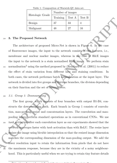
Table 1: Composition of Warwick-QU data set.

Histologic Grade Number of images

Training Test A Test B

Benign 37 33 4

Malignant 48 27 16

3. The Proposed Network

210

The architecture of proposed Micro-Net is shown in Figure 6. In the case

of fluorescence images, the input to the network consists of two features, i.e.,

membrane and nuclear marker images, whereas in the case of H&E images

the input to the network is a stain normalised RGB image. We perform stain

normalisation2_{using the method proposed by (Reinhard et al. (2001)) to reduce} 215

the effect of stain variation from different labs and staining conditions. In

both cases, the network performes batch normalisation at the input layer. The

network is divided into five groups and thirteen branches, the division depending

on their function and the set of layers/filters.

3.1. Group 1: Downsampling

220

The first group, which consists of four branches with output B1-B4,

con-structs the downsampling path. Each branch in Group 1 consists of

convolu-tion, pooling, resize and concatenation layers. The convolution and

max-pooling layers perform standard operations as in conventional CNNs. We use

tanhactivation after each convolution layer as our experiments showed that the

225

network converges faster withtanh activation than with ReLU. The resize layer

resizes the image using bicubic interpolation so that the resized image dimension

matches the corresponding dimension of the max-pooling output. We add the

lower resolution input to retain the information from pixels that do not have

the maximum response, because they are in the vicinity of a noisy

neighbour-230

hood. This is particularly useful when we are trying to retain tiny feature details

ACCEPTED MANUSCRIPT

(a)

(b)

Figure 6: The proposed Micro-Net architecture. (a) Micro-Net-252 & (b) Micro-Net-508.

ignored during the max-pooling operation, for example, when trying to detect

cells with boundary markers having extreme intensities, even for individual cells

as shown in Figure 3. Another aspect of the resizing operation is to train the

network on different sized cells/nuclei and glands as explained in Section 2. The

235

ACCEPTED MANUSCRIPT

(64) are obtained by performing convolutions only on the resized image. The

following branches in Group 1 double the feature depth of the previous branch

but follow the same protocol in generating the branch output. The only

differ-240

ence is that B1 performs batch normalisation at the input and the resize layer

whereas B2-B4 perform batch normalisation at the resize layer only.

3.2. Group 2: Bridge

Group 2, consisting of B5, bridges the connection between the downsampling

and upsampling paths, whose architecture is very similar to conventional CNN

245

architectures.

3.3. Group 3: Upsampling

Group 3 forms the upsampling path and consists of branches B6, B7, B8 &

B9. Each of these branches take two inputs, one from the previous branch and

one from the branch with the closest feature dimension in the downsampling

250

path. The output of each branch is double in height and width and half the depth

of the previous branch. The second input is added from the downsampling path

for better localization and to capture context information as in (Ronneberger

et al. (2015)). It also passes the convolution only features to the upsampling

path, which helps to learn from features which do not have maximum response

255

in the downsampling path. Compared to U-Net (Ronneberger et al. (2015)),

we add additional deconvolution layers instead of cropping the feature from the

downsampling path. This allows us to produce a segmentation map of the same

size as the input image and an overlap-tile strategy is not required. It also

reduces the number of patches required to produce the desired segmentation

260

output thus removing computational steps.

3.4. Group 4 & 5: Auxiliary and Main Output

Group 4 & 5 generate the auxiliary and main output and calculate the

ACCEPTED MANUSCRIPT

265

are fed into the main output branch. The output branch concatenates feature

masks and performs convolution followed by softmax classification to get the

segmentation output mappo(x) wherexrepresents a pixel location. The output

of branches B7-B9 are of different resolutions and so the deconvolution layer in

each of the auxiliary branches is set to generate the output of the same size

270

(Chen et al. (2017)). The deconvolution is followed by a convolution layer

which produces the auxiliary feature mask. Each of the auxiliary feature masks

is followed by a dropout layer (set to 50%) and the convolution layer followed

by softmax classification to get the auxiliary outputs (pa1(x),pa2(x),pa3(x)).

3.5. Modifications for Gland Segmentation

275

For gland segmentation we slightly modified the network to train on a bigger

patch size as shown in Figure 6(b). We doubled the input size to incorporate

larger context to take account of the larger size of glands as compared individual

cells. This modified architecture consists of five groups and fourteen branches

where all five groups and the corresponding branches perform the same tasks

280

as in Figure 6(a). However, the architecture of group 2 was slightly modified to

learn deep features by adding an additional branch that performs deconvolution

followed by convolution. The additional branch in group 2 was added so that the

smallest feature patch size is (8×8) in line with the Micro-Net 252 architecture.

The rest of the architecture remains the same except for the size of input/output

285

for each branch.

3.6. Loss Function

For training, we calculate weighted cross entropy loss for the main output

(lo) and the auxiliary outputs (la1,la2,la3) as

lk=

X

x∈Ω

w(x) log(pk(x)(x)) (1)

ACCEPTED MANUSCRIPT

290

(Ronneberger et al. (2015)). The total loss (l) is calculated by combining

aux-iliary and main loss by usingl =lo+ (la1+la2+la3)/epoch whereepoch >0

represents the number of training passes already made through the data. This

strategy reduces exponentially the contribution of auxiliary losses for a higher

epoch, avoiding reduction of the contribution by large steps (Chen et al. (2017)).

295

3.7. Data Augmentation

As deep learning algorithms require large amounts of data for training, we

augment the data using barrel, pincushion and moustache distortion. While

adjusting parameters we made sure by visual examination that the distortions

created by these parameters were realistic and not too strong. For cell

segmen-300

tation on fluorescence imaging data, we augmented the data by adding white

Gaussian noise with mean 0 and variance in the range 0.0007 to 0.001, where

for each patch the value of variance was randomly selected. For nuclear and

gland segmentation we introduced Gaussian blur with a Gaussian filter of size

12×12, with σ ranging from 0.2 to 2. The value σ was randomly selected

305

for each patch. In addition we rotate, and flip the images left, right, up and

down. To train the network for cell/nuclear (gland) segmentation, we first

ex-tract 300×300 (600×600) patches from the training data. If the size of image is smaller than 300 (600) in height or width, we symmetrically pad the image to

increase its size. During training the network picks these patches in a random

310

order for eachepoch, choosing centres for the patches at random locations, and

then cropping them to a size of 252×252 (508×508) patch before inputting. The proposed network was implemented using TensorFlow v0.12 (Abadi et al.

(2015)). We start with a learning rate (lr = 0.001) and reduce it according to

lr = 0.001/(10(epoch/5)_{), which reduces the learning rate by a factor of 10 for}

315

ACCEPTED MANUSCRIPT

Figure 7: Segmentation results, ground truth in red, output of the algorithm in green and overlap between ground truth and output of algorithm in yellow. Top row: Exocrine region.

Bottom row: Endocrine region. Columns (left to right) are output from FCN8, U-Net, DCAN

and Micro-Net architectures.

4. Results and Discussion

4.1. Multiplexed Fluorescence Imaging Data

Our image data consists of 10 images of size 2048×2048 pixels (11,163 cells) of which 6 images (with approximately 60% i.e., 6,641 cells) are used for

train-320

ing and 4 images (with the remaining 40% i.e., 4,522 cells) for testing. During

training, we used 20% of the data for validation. We compare our results with

the state-of-the-art FCN8 (Shelhamer et al. (2017)), DCAN (Chen et al. (2017))

and U-Net (Ronneberger et al. (2015)) networks. To remove the bias we trained

all the networks on the same training data obtained after augmentation. We

325

used the authors’ implementation of FCN8 and trained it for our data, whereas

DCAN and U-Net were implemented in TensorFlow. The weights for the

pro-posed network were initialised with truncated Gaussian and the network was

trained for 25 epochs. The checkpoint was chosen based on the minimum

vali-dation loss. For U-Net and DCAN, we ran the network for 30 epochs but the

330

criteria for choosing the trained checkpoint file was thesame (i.e., best

ACCEPTED MANUSCRIPT

DCAN is designed to learn the contour features and performed better

segmen-tation of the cells in the exocrine region but performed poorly with smaller

335

sized cells in the endocrine region. U-Net performed better than both FCN and

DCAN but missed the cells with weaker boundaries. The proposed Micro-Net

method, performed better in the presence of variable intensities and variable

size/shape of the cells. The output in Figure 7 was post-processed for all the

algorithms using area opening (100 pixels) and hole filling operations to get

340

the final output score in Table 2. For quantitative analysis, we used measures

which include Dice coefficient, F1 score, object Dice, pixel accuracy and object

Hausdorff (Sirinukunwattana et al. (2017)). Better results correspond to smaller

Hausdorff distance and all other measures larger. The quantitative results are

shown in Table 2 which show that the proposed Micro-Net method outperforms

345

the state-of-the-art deep learning approaches with at least 3-4% margin in terms

of average Dice, F1 score, object Dice, pixel accuracy and object Hausdorff. We

modified the FCN8 algorithm (FCN8W) by introducing weighted loss

(Ron-neberger et al. (2015)) to improve segmentation of individual cells. FCN8W

improved F1, object Dice, pixel accuracy and object Hausdorff but failed to

350

increase the Dice coefficient. In addition, we add results for Micro-Net–_where

we removed the multi-resolution input and the bypass layers. The results are

slightly better compared to U-Net but not better than Micro-Net supporting

the suggested changes in the design.

In addition to the above experiments we tested all the network architectures

355

for their robustness to various levels of white Gaussian noise by controlling the

SNR and generating the output for various network architectures. For this

purpose we did not retrain the networks but used the already trained models as

above. The values for Dice, F1, object Dice, pixel accuracy and object Hausdorff

for various SNR values are given in Table 3, 4, 5, 6 and 7 respectively. For Dice

360

coefficient, FCN8 and U-Net drop to 73% whereas the proposed method drops

to 78%. However, DCAN shows a different behaviour and increases the Dice

ACCEPTED MANUSCRIPT

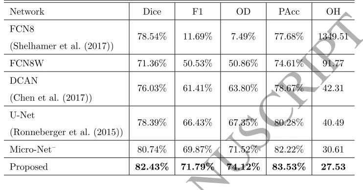
Table 2: Quantitative results for cell segmentation in terms of Dice coefficient, F1 score, Object Dice (OD), Pixel Accuracy (Acc) & Object Hausdorff (OH).

Network Dice F1 OD PAcc OH

FCN8

(Shelhamer et al. (2017)) 78.54% 11.69% 7.49% 77.68% 1349.51

FCN8W 71.36% 50.53% 50.86% 74.61% 91.77

DCAN

(Chen et al. (2017)) 76.03% 61.41% 63.80% 78.67% 42.31

U-Net

(Ronneberger et al. (2015)) 78.39% 66.43% 67.35% 80.28% 40.49

Micro-Net– _{80.74% 69.87% 71.52% 82.22% 30.61}

Proposed 82.43% 71.79% 74.12% 83.53% 27.53

networks drop to below 65% at 1dB where the proposed network retains the

top position. The trend was similar with object Dice as well where the first

365

position was retained by the proposed network. In terms of pixel accuracy,

the proposed method dropped roughly 4% from 20dB to 1dB. DCAN however

showed similar trend to Dice values i.e., increased pixel accuracy with increasing

noise content. This is an interesting result, but if we carefully observe Dice and

pixel accuracy both depend only on the pixels that are in agreement, whereas

370

object Dice only takes into account the pixels which belong to the ground truth.

Similarly, the F1 score takes into account not only true positives but also false

positives. With increasing noise content, DCAN lost some of the false positives

causing more pixels not belonging to the cellular region to agree. This increased

pixel accuracy and Dice while simultaneously decreasing object Dice and the F1

375

score. Object Hausdorff is a measure of similarity of the shape of cell boundaries

and is lower for better performance. Here the author’s implementation of FCN

produced very high values, whereas with weighted loss (FCN8W) the values were

in a comparable range. Additionally FCN8W values improved with increasing

noise due to the resulting loss of many cell segmentations. U-Net increased 55

ACCEPTED MANUSCRIPT

performed better as it is designed to match the contours and only increased

12 points with increased noise content. However, the proposed network only

increased 6 points showing the stability of the network and it’s robustness to

the noise. It is important to note here that Micro-Net– _{shows the steepest} 385

decline in performance (in terms of Dice, F1, object Dice and pixel accuracy)

with increasing noise content compared to U-Net, DCAN and Micro-Net. The

decline is not much in the case of object Hausdorff as Micro-Net–_{uses the}

multi-resolution output, and therefore shows robust shape similarity (on segmented

cells) as shown by DCAN (which also utilises multi-resolution output). This

390

further emphasises the role of multi-resolution input and the bypass layers.

Overall, the proposed network outperformed the recent deep learning models

for various levels of noise in terms of Dice, the F1 score, object Dice, pixel

accuracy and object Hausdorff. In terms of computation time, on average the

network takes 2.50 sec/batch for training and 0.39 sec/batch for testing a batch

395

of 5 images on a Windows10 machine with Intel Xeon E5-2670 v2 CPU, TitanX

Maxwell GPU and 96 GB RAM. For 25 epochs, it took around 4.5 days to train

the network.

Table 3: Quantitative results for cell segmentation of state-of-the-art algorithms in terms of Dice coefficient for various SNR values.

Network 20dB 15dB 10dB 5dB 3dB 1dB

FCN8

(Shelhamer et al. (2017)) 77.55% 76.24% 76.97% 76.47% 75.26% 73.66%

FCN8W 71.56% 71.53% 71.39% 70.56% 69.36% 66.88%

DCAN

(Chen et al. (2017)) 77.18% 77.95% 78.92% 79.82% 79.91% 79.40%

U-Net

(Ronneberger et al. (2015)) 76.58% 76.61% 76.29% 75.59% 74.99% 73.45%

Micro-Net– _{81.35% 81.42% 80.72% 78.30% 76.04% 72.33%}

ACCEPTED MANUSCRIPT

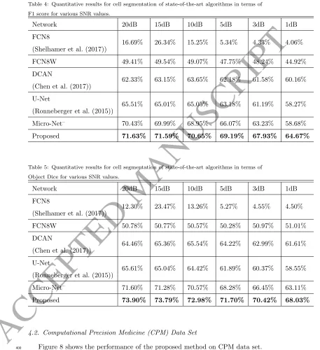
Table 4: Quantitative results for cell segmentation of state-of-the-art algorithms in terms of F1 score for various SNR values.

Network 20dB 15dB 10dB 5dB 3dB 1dB

FCN8

(Shelhamer et al. (2017)) 16.69% 26.34% 15.25% 5.34% 4.33% 4.06%

FCN8W 49.41% 49.54% 49.07% 47.75% 48.24% 44.92%

DCAN

(Chen et al. (2017)) 62.33% 63.15% 63.65% 62.18% 61.58% 60.16%

U-Net

(Ronneberger et al. (2015)) 65.51% 65.01% 65.05% 63.18% 61.19% 58.27%

Micro-Net– _{70.43% 69.99% 68.95% 66.07% 63.23% 58.68%}

Proposed 71.63% 71.59% 70.65% 69.19% 67.93% 64.67%

Table 5: Quantitative results for cell segmentation of state-of-the-art algorithms in terms of

Object Dice for various SNR values.

Network 20dB 15dB 10dB 5dB 3dB 1dB

FCN8

(Shelhamer et al. (2017)) 12.30% 23.47% 13.26% 5.27% 4.55% 4.50%

FCN8W 50.78% 50.77% 50.57% 50.28% 50.97% 51.01%

DCAN

(Chen et al. (2017)) 64.46% 65.36% 65.54% 64.22% 62.99% 61.61%

U-Net

(Ronneberger et al. (2015)) 65.61% 65.04% 64.42% 61.89% 60.37% 58.55%

Micro-Net– _{71.60% 71.28% 70.57% 68.28% 66.45% 63.11%}

Proposed 73.90% 73.79% 72.98% 71.70% 70.42% 68.03%

4.2. Computational Precision Medicine (CPM) Data Set

Figure 8 shows the performance of the proposed method on CPM data set.

400

ACCEPTED MANUSCRIPT

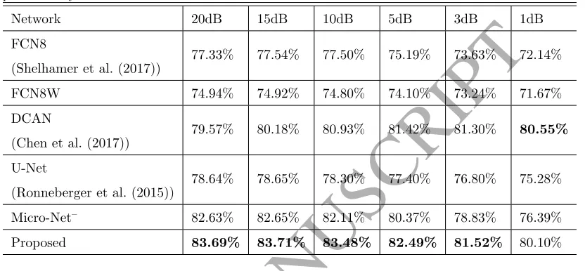
Table 6: Quantitative results for cell segmentation of state-of-the-art algorithms in terms of pixel accuracy for various SNR values.

Network 20dB 15dB 10dB 5dB 3dB 1dB

FCN8

(Shelhamer et al. (2017)) 77.33% 77.54% 77.50% 75.19% 73.63% 72.14%

FCN8W 74.94% 74.92% 74.80% 74.10% 73.24% 71.67%

DCAN

(Chen et al. (2017)) 79.57% 80.18% 80.93% 81.42% 81.30% 80.55%

U-Net

(Ronneberger et al. (2015)) 78.64% 78.65% 78.30% 77.40% 76.80% 75.28%

Micro-Net– _{82.63% 82.65% 82.11% 80.37% 78.83% 76.39%}

Proposed 83.69% 83.71% 83.48% 82.49% 81.52% 80.10%

Table 7: Quantitative results for cell segmentation of state-of-the-art algorithms in terms of

object Hausdorff for various SNR values.

Network 20dB 15dB 10dB 5dB 3dB 1dB

FCN8

(Shelhamer et al. (2017)) 1171.08 604.18 1176.88 1618.90 1700.83 1589.12

FCN8W 88.55 90.42 86.99 84.24 81.03 66.30

DCAN

(Chen et al. (2017)) 42.20 41.16 42.32 47.72 50.92 54.21

U-Net

(Ronneberger et al. (2015)) 55.53 63.53 62.50 85.48 97.49 100.15

Micro-Net– _{31.42 32.13 32.85 33.62 33.91 35.13}

Proposed 27.98 28.35 29.64 30.73 31.69 33.84

(HNSCC), lower grade glioma (LGG), non-small cell lung cancer (NSCLC) &

glioblastoma multiforme (GBM) respectively. Column 1 shows H & E image

with ground truth outlined for nuclear segmentation. Column 2 shows an RGB

composite image with ground truth in green and output of U-Net in red and

405

com-ACCEPTED MANUSCRIPT

in red and the overlap in yellow. In HNSCC, on the lower left corner we can

observe red cells, that are segmented by the proposed algorithm, but not picked

during ground truth marking. On the other hand, on the top right, the

algo-410

rithm undersegments, due to the relatively weak signal of the nuclei. In LGG,

the proposed algorithm seems to oversegment where the ground truth might

have been mistakenly marked on the nucleolus rather than on the nucleus of

the cell. The algorithm seems to be struggling in these kinds of regions in

NSCLC as well, where it missed segmenting the nuclei under darker shades.

415

In GBM, the proposed algorithm misses a few cells with fainter nuclei.

Over-all the performance of the algorithm seems good; however it seems to struggle

with nuclei under multiple shades. U-Net on the other hand shows more red

in all cases demonstrating oversegmentation. This is particularly noticeable in

NSCLC where there seems to be a strong cytoplasmic shade. Micro-Net

strug-420

gles in these circumstances but performs much better than U-Net due to its

robustness. We quantitatively measure the performance of segmentation using

two evaluation metrics as selected by the contest organisers (CPM), namely

Tra-ditional Dice (Dice 1) and Ensemble Dice (Dice 2). Dice 1 measures the overlap

between the ground truth and the prediction, whereas Dice 2 also penalises the

425

prediction if there is a mismatch in the way segmentation regions are split. The

overall score is then computed as the average of the two Dice coefficients. We

compare our results with FCN8 (Shelhamer et al. (2017)), U-Net (Ronneberger

et al. (2015)), SAMS-Net (Graham and Rajpoot (2018)) and the submissions

in the competition. The results in Table 8 show that our method not only

out-430

performs the results of contest winners but also recent deep learning methods

such as SAMS-Net (Graham and Rajpoot (2018)).

4.3. Gland Segmentation Challenge (GLaS) Data Set

We used 85 images for training and 80 for testing, where 60 of the test images

correspond to Test set A and the remaining 20 to Test set B. For quantitative

435

ACCEPTED MANUSCRIPT

Figure 8: Top to Down: (1) HNSCC, (2) LGG, (3) NSCLC, (4) GBM. Left to Right: (1) H & E image with ground truth outlined for nuclear segmentation, (2) RGB composite image with

ground truth in green and output of U-Net in red, (3) RGB composite image with ground

ACCEPTED MANUSCRIPT

Table 8: Cell segmentation results on CPM contest data set using evaluation metrics Dice 1 and Dice 2 as selected by the organisers.

Method Dice 1 Dice 2 Score Rank

Proposed 0.857 0.796 0.827 1

SAMS-Net (Graham and Rajpoot (2018)) 0.855 0.769 0.812 2

U-Net (Ronneberger et al. (2015)) 0.837 0.741 0.789 3

vuquocdang - - 0.783 4

brisker - - 0.773 5

FCN8 (Shelhamer et al. (2017)) 0.829 0.697 0.763 6

Schwarz - - 0.703 7

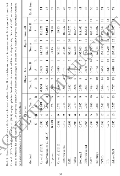
object Hausdorff (Sirinukunwattana et al. (2017)). In the case of Hausdorff

distance lower values are better; for other measures higher are better. The

quantitative results are given in Table 9 which shows that our method produces

competitive results compared to the state-of-the-art algorithms from the contest

440

and ranks third after the recently proposed (Xu et al. (2017); Manivannan et al.

(2018)) according the rank sum criteria set by the organisers. Xu et al. (2017)

and Manivannan et al. (2018) employ optimised handcrafted features in addition

to deep learning. Xu et al. (2017) on the other hand is heavily optimised for

gland segmentation. Our algorithm employs only deep learning and is being

445

proposed as a generic approach for cell, nuclear and gland segmentation, easily

implemented using existing libraries optimised for GPU usage, which reduces the

computational cost. Nevertheless, the proposed method performs competitively

against recently proposed approaches and beats the conference version of Xu

et al. (2016). Compared to the results of the contest on test A, the proposed

450

algorithm performed best in terms of F1 and object Dice but ranked third and

fifth on test B. In terms of object Hausdorff, which measures the shape similarity,

it ranked second after CUMedVision2 (Chen et al. (2017)) on test A and Xu et al.

(2016) on test B. Lower F1 and object Dice on test B suggests that our method

missed more glands in malignant cases, whereas lower Hausdorff suggests higher

ACCEPTED MANUSCRIPT

results of the algorithm for sample images in Figure 5 are shown in Figure 9,

where for each pair the image on first and second column show ground truth

in green, output of DCAN (contest winner, the results were obtained from the

contest organisers) and the proposed algorithm respectively in red and overlap of

460

ground truth and output of algorithm in yellow. The image on the right shows

the output of the proposed algorithm overlaid on the sample image. These

results show that our algorithm clearly misses a few glands on the boundary of

the image for which there is insufficient information. In the second row, it merges

the glands at the bottom of the image and misses one gland. In malignant cases

465

the algorithm seems to be rather ‘conservative’ in its approach when marking

the boundary of glands. It can be observed in the third row for the two large

glands at the bottom and in the fourth row for the smaller gland in the middle.

All these glands show significant green inside the ground truth boundary, which

at first suggests that the algorithm segmented the gland well inside the ground

470

truth marking for the gland. However, when carefully observed in the overlay

with the sample images the algorithm is faithfully following the boundary with

tumor cells. For the large gland on the top right in third row the algorithm

‘oversegments’ the gland compared to the ground truth but again, looking at

the overlay with the sample image, the algorithm has included tumor cells in

475

the segmentation. Overall the algorithm performs a good job in segmenting the

glands but needs to improve on the glands at the boundary of a patch. This

limitation could be overcome by using overlapping patches from the whole slide

and then merging the results. Compared to DCAN (first column), the proposed

algorithm shows better overlap with the ground truth. It can be observed that

480

DCAN is sensitive to white spaces and certain architecture in benign cases

where it segments false regions. This can be clearly observed in cases from row

2, 3 & 4 and column 1. In the fourth row, it joins two glands together and

under segments the smaller gland in the middle. It can also be observed that

similar to the proposed algorithm, DCAN misses the glands at the boundary

485

ACCEPTED MANUSCRIPT

Figure 9: Results of the proposed network for sample images in Figure 5. First and second column show RGB composite images with output of the DCAN (Chen et al. (2017)) and the

proposed algorithm respectively in red, ground truth in green and overlap of ground truth

and output in yellow. The image in the third column shows the output of the proposed method overlaid on the sample image. The results for DCAN were obtained from the contest

organisers.

in terms of qualitative and quantitative results.

5. Conclusions

In multi-channel fluorescence microscopy, cell segmentation can help to build

molecular profiles of individual cells. However, images captured using

fluores-490

cence microscopy contain very weak and variable intensities that make it difficult

ACCEPTED MANUSCRIPT

seg-mentation. In tumour histology slides, the morphology of nuclei and nuclear

pleomorphism can help in making a diagnosis and in studying the tumour

mi-495

croenvironment but nuclear segmentation is difficult due to varying shape, size,

chromatin structure and clumped nuclei. Similarly morphology of glands can

help the pathologist to grade the cancer but it is also very challenging due

to texture, size and structure of the glands. All these tasks require

sophisti-cated segmentation algorithms. We have presented a deep learning architecture

500

named Micro-Net that can be used to segment cells/nuclei and glands in

fluores-cence and H&E stained images with slight tuning of theinputparameters. The

proposed architecture allows the network to visualise input and output at

mul-tiple resolutions. The extra convolutional layers bypass the max-pooling layer,

thus allowing the network to better train its parameters for weak features in

505

addition to the strongly observed feature sets. This has been demonstrated by

the robustness of algorithm to varying level of noise in fluorescence image data.

Intermediate connections between the layers allow context and localization to

be retained. The qualitative and quantitative results show that the Micro-Net

architecture outperforms recently published deep learning approaches. We will

510

make the fluorescence image data set publicly available subject to publication of

this manuscript. The other two data sets we used in this paper are already

pub-licly available. We showed that the proposed algorithm produces competitive

results compared to the state-of-the-art. The results produced by the algorithm

can be extended to build molecular profile in multiplexed fluorescence images,

515

grade cancer or study tumour microenvironment.

6. Acknowledgements

We are grateful to the BBSRC UK for supporting this study through project

ACCEPTED MANUSCRIPT

520

Computational precision medicine nuclei segmentation challenge website.http:

//miccai.cloudapp.net/competitions/57.

Abadi M, Agarwal A, Barham P, Brevdo E, Chen Z, Citro C, Corrado GS, Davis

A, Dean J, Devin M, Ghemawat S, Goodfellow I, Harp A, Irving G, Isard M,

Jia Y, Jozefowicz R, Kaiser L, Kudlur M, Levenberg J, Man´e D, Monga R,

525

Moore S, Murray D, Olah C, Schuster M, Shlens J, Steiner B, Sutskever

I, Talwar K, Tucker P, Vanhoucke V, Vasudevan V, Vi´egas F, Vinyals O,

Warden P, Wattenberg M, Wicke M, Yu Y, Zheng X. TensorFlow:

Large-scale machine learning on heterogeneous systems. 2015. URL:https://www.

tensorflow.org/; software available from tensorflow.org.

530

Awan R, Sirinukunwattana K, Epstein D, Jefferyes S, Qidwai U, Aftab Z,

Mujeeb I, Snead D, Rajpoot N. Glandular morphometrics for objective

grading of colorectal adenocarcinoma histology images. Scientific reports

2017;7(1):16852. doi:10.1038/s41598-017-16516-w.

Bergeest J, Rohr K. Efficient globally optimal segmentation of cells in

fluores-535

cence microscopy images using level sets and convex energy functionals.

Med-ical image analysis 2012;16(7):1436–44. doi:10.1016/j.media.2012.05.012.

Carpenter AE, Jones TR, Lamprecht MR, Clarke C, Kang IH, Friman O,

Guertin DA, Chang JH, Lindquist RA, Moffat J, et al. Cellprofiler: image

analysis software for identifying and quantifying cell phenotypes. Genome

540

biology 2006;7(10):R100. doi:10.1186/gb-2006-7-10-r100.

Chen H, Qi X, Yu L, Dou Q, Qin J, Heng PA. Dcan: Deep contour-aware

net-works for object instance segmentation from histology images. Medical Image

Analysis 2017;36(Supplement C):135 –46. doi:10.1016/j.media.2016.11.

004.

545

Cohen A, Rivlin E, Shimshoni I, Sabo E. Memory based active contour

Com-ACCEPTED MANUSCRIPT

compmedimag.2014.12.006.

Dimopoulos S, Mayer CE, Rudolf F, Stelling J. Accurate cell segmentation in

mi-550

croscopy images using membrane patterns. Bioinformatics 2014;30(18):2644–

51. doi:10.1093/bioinformatics/btu302.

Farjam R, Soltanian-Zadeh H, Jafari-Khouzani K, Zoroofi RA. An image

anal-ysis approach for automatic malignancy determination of prostate

patho-logical images. Cytometry Part B: Clinical Cytometry 2007;72B(4):227–40.

555

doi:10.1002/cyto.b.20162.

Graham S, Rajpoot NM. Sams-net: Stain-aware multi-scale network for

instance-based nuclei segmentation in histology images. In: 2018 IEEE 15th

International Symposium on Biomedical Imaging (ISBI 2018). 2018. p. 590–4.

doi:10.1109/ISBI.2018.8363645.

560

Gunduz-Demir C, Kandemir M, Tosun AB, Sokmensuer C. Automatic

seg-mentation of colon glands using object-graphs. Medical image analysis

2010;14(1):1–12. doi:10.1016/j.media.2009.09.001.

He K, Zhang X, Ren S, Sun J. Deep residual learning for image recognition. In:

Proceedings of the IEEE conference on computer vision and pattern

recogni-565

tion. 2016. p. 770–8. doi:10.1109/CVPR.2016.90.

Kraus OZ, Ba JL, Frey BJ. Classifying and segmenting microscopy images with

deep multiple instance learning. Bioinformatics 2016;32(12):i52–9. doi:10.

1093/bioinformatics/btw252.

Li G, Raza SEA, Rajpoot NM. Multi-resolution cell orientation congruence

de-570

scriptors for epithelium segmentation in endometrial histology images.

Med-ical Image Analysis 2017;37:91 – 100. doi:10.1016/j.media.2017.01.006.

Li G, Sanchez V, Nagaraj P, Khan S, Rajpoot N. A novel multitarget

track-ing algorithm for myosin vi protein molecules on actin filaments in tirfm

se-quences. Journal of Microscopy 2015;260(3):312–25. doi:10.1111/jmi.12299.

ACCEPTED MANUSCRIPT

gland segmentation with hand-crafted and deep convolutional features. IEEE

Transactions on Medical Imaging 2018;37(1):210–21. doi:10.1109/TMI.2017.

2750210.

Meijering E. Cell segmentation: 50 years down the road. Signal Processing

580

Magazine, IEEE 2012;29(5):140–5. doi:10.1109/MSP.2012.2204190.

Naik S, Doyle S, Agner S, Madabhushi A, Feldman M, Tomaszewski J.

Au-tomated gland and nuclei segmentation for grading of prostate and breast

cancer histopathology. In: Biomedical Imaging: From Nano to Macro, 2008.

ISBI 2008. 5th IEEE International Symposium on. IEEE; 2008. p. 284–7.

585

doi:10.1109/ISBI.2008.4540988.

Nguyen K, Sarkar A, Jain AK. Structure and context in prostatic gland

seg-mentation and classification. In: Medical Image Computing and

Computer-Assisted Intervention–MICCAI 2012. Springer; 2012. p. 115–23. doi:10.1007/

978-3-642-33415-3_15.

590

Nosrati MS, Hamarneh G. Local optimization based segmentation of

spatially-recurring, multi-region objects with part configuration constraints. IEEE

transactions on medical imaging 2014;33(9):1845–59. doi:10.1109/TMI.2014.

2323074.

Qaiser T, Tsang YW, Epstein D, Rajpoot N. Tumor segmentation in whole

595

slide images using persistent homology and deep convolutional features. In:

Annual Conference on Medical Image Understanding and Analysis. Springer;

2017. p. 320–9. doi:10.1007/978-3-319-60964-5_28.

Raza SEA, Cheung L, Epstein D, Pelengaris S, Khan M, Rajpoot NM.

Mimo-net: A multi-input multi-output convolutional neural network for cell

seg-600

mentation in fluorescence microscopy images. In: 2017 IEEE 14th

Inter-national Symposium on Biomedical Imaging (ISBI 2017). 2017a. p. 337–40.

ACCEPTED MANUSCRIPT

MI-MONet: Gland Segmentation Using Multi-Input-Multi-Output Convolutional

605

Neural Network; Cham: Springer International Publishing. p. 698–706.

doi:10.1007/978-3-319-60964-5_61.

Raza SEA, Humayun A, Abouna S, Nattkemper TW, Epstein DB, Khan M,

Rajpoot NM, et al. RAMTaB: robust alignment of multi-tag bioimages. PLoS

ONE 2012;7(2):e30894. doi:10.1371/journal.pone.0030894.

610

Raza SEA, Langenk¨amper D, Sirinukunwattana K, Epstein D, Nattkemper

TW, Rajpoot NM. Robust normalization protocols for multiplexed

fluo-rescence bioimage analysis. BioData Mining 2016;9(1):11. doi:10.1186/

s13040-016-0088-2.

Reinhard E, Adhikhmin M, Gooch B, Shirley P. Color transfer between images.

615

IEEE Computer graphics and applications 2001;21(5):34–41.

Ronneberger O, Fischer P, Brox T. U-net: Convolutional networks for

biomedical image segmentation. In: International Conference on

Medi-cal Image Computing and Computer-Assisted Intervention. 2015. p. 234–41.

doi:10.1007/978-3-319-24574-4_28.

620

Sadanandan SK, Ranefall P, Le Guyader S, W¨ahlby C. Automated training of

deep convolutional neural networks for cell segmentation. Scientific reports

2017;7(1):7860. doi:10.1038/s41598-017-07599-6.

Schubert W, Bonnekoh B, Pommer AJ, Philipsen L, B¨ockelmann R, Malykh Y,

Gollnick H, Friedenberger M, Bode M, Dress AW. Analyzing proteome

topol-625

ogy and function by automated multidimensional fluorescence microscopy.

Nature biotechnology 2006;24(10):1270. doi:10.1038/nbt1250.

Shelhamer E, Long J, Darrell T. Fully convolutional networks for semantic

seg-mentation. IEEE Transactions on Pattern Analysis and Machine Intelligence

2017;39(4):640–51. doi:10.1109/TPAMI.2016.2572683.

ACCEPTED MANUSCRIPT

LY, Matuszewski BJ, Bruni E, Sanchez U, et al. Gland segmentation in

colon histology images: The glas challenge contest. Medical image analysis

2017;35:489–502. doi:10.1016/j.media.2016.08.008.

Sirinukunwattana K, Snead DR, Rajpoot NM. A stochastic polygons model for

635

glandular structures in colon histology images. IEEE transactions on medical

imaging 2015;34(11):2366–78. doi:10.1109/TMI.2015.2433900.

Song Y, Tan EL, Jiang X, Cheng JZ, Ni D, Chen S, Lei B, Wang T.

Accu-rate cervical cell segmentation from overlapping clumps in pap smear images.

IEEE Transactions on Medical Imaging 2017;36(1):288–300. doi:10.1109/

640

TMI.2016.2606380.

Veta M, Van Diest PJ, Kornegoor R, Huisman A, Viergever MA, Pluim JP.

Au-tomatic Nuclei Segmentation in H&E Stained Breast Cancer Histopathology

Images. PLoS ONE 2013;8(7):e70221. doi:10.1371/journal.pone.0070221.

Wu HS, Xu R, Harpaz N, Burstein D, Gil J. Segmentation of intestinal gland

645

images with iterative region growing. Journal of Microscopy 2005;220(3):190–

204. doi:10.1111/j.1365-2818.2005.01531.x.

Xu Y, Li Y, Liu M, Wang Y, Lai M, Eric I, Chang C. Gland instance

segmen-tation by deep multichannel side supervision. In: International Conference

on Medical Image Computing and Computer-Assisted Intervention. Springer;

650

2016. p. 496–504. doi:10.1007/978-3-319-46723-8_57.

Xu Y, Li Y, Wang Y, Liu M, Fan Y, Lai M, Chang EIC. Gland instance

segmentation using deep multichannel neural networks. IEEE Transactions

on Biomedical Engineering 2017;64(12):2901–12. doi:10.1109/TBME.2017.

2686418.

655

Yang X, Li H, Zhou X. Nuclei segmentation using marker-controlled watershed,

ACCEPTED MANUSCRIPT

doi:10.1109/TCSI.2006.884469.

Yuan Y, Failmezger H, Rueda OM, Ali HR, Gr¨af S, Chin SF, Schwarz RF,

660

Curtis C, Dunning MJ, Bardwell H, et al. Quantitative image analysis of

cel-lular heterogeneity in breast tumors complements genomic profiling. Science

translational medicine 2012;4(157):157ra143–. doi:10.1126/scitranslmed.