The Multimode Covering Location Problem.
Fabio Colombo
∗Roberto Cordone
†Guglielmo Lulli
‡July 1, 2015
Abstract
In this paper we introduce theMultimode Covering Location Problem. This is a generalization of the Maximal Covering Location Problem that consists in locating a given number of facilities of different types with a limitation on the number of facilities sharing the same site.
The problem is challenging and intrinsically much harder than its basic version. Nevertheless, it admits a constant factor approximation guaran-tee, which can be achieved combining two greedy algorithms. To improve the greedy solutions, we have developed aVariable Neighborhood Search approach, based on an exponential-size neighborhood. This algorithm computes good quality solutions in short computational time. The viabil-ity of the approach here proposed is also corroborated by a comparison with a Heuristic Concentration algorithm, which is presently the most effective approach to solve large instances of the Maximal Covering Loca-tion Problem.
1
Introduction.
A facility location problem consists in placing a number of facilities to serve a set of demand centers, whose positions are known, while optimizing a given objective function. The problem admits several variants, based on the objective of the decision maker and on the application setting. For a complete taxonomy of facility location problems, the interested reader may refer to ReVelleet al.[35]. In this paper we focus on a generalized version of the Maximal Covering Location Problem (MCLP), first proposed by Church and ReVelle [8]. The
MCLP belongs to the class of discrete location problems, i.e., problems with a finite set of demand centers and a finite set of candidate locations. TheMCLP
does not require all the demand centers to be served: its purpose is to locate a given number of facilities maximizing the number, or the total weight, of
∗University of Milano, Department of Computer Science, via Comelico 39, 20135 Milano,
Italy,[email protected]
†University of Milano, Department of Computer Science, via Comelico 39, 20135 Milano,
Italy,[email protected]
‡University of Milano “Bicocca”, Department of Informatics, Systems and Communication,
the served demand centers. Because of its wide applicability in the real world, especially in the planning of service and emergency facilities, the MCLP is a well-studied problem. Chung [7] reviewed several other applications of the
MCLP, such as data abstraction, stock selection and classification problems. Other interesting applications are those described by Dwyer and Evans [18] for the selection of mailing lists, Daskin et al. [14] for flexible manufacturing, Hougland and Stephens [28] for air pollution control and Melo et al. [30] for supply chain management.
Since its proposal, theMCLP has been generalized in different ways. Berman et al. [5] reviewed gradual cover models, cooperative cover models and variable radius models. Ghiani et al. [25] introduced a capacitated plant location problem where multiple facilities can be opened in the same site. Rajagopalan, Saydam and Xiao [34] considered a multiperiod set covering location model in the field of application of emergency medical services. Dell’Olmo et al. [16] tackled the optimal location of intersection safety cameras on an urban traffic network to minimize the impact of car accidents, through a multiperiod variant of maximal covering location.
In this paper, we present the Multimode Covering Location Problem ( MM-CLP). This problem consists in placing a given number of facilities of different types (hereafter called modes) to serve demand centers that require different types of service. The goal is to maximize the demand coverage over all the considered modes. An additional restriction with respect to theMCLP is that only a limited number of different modes can be activated in each candidate facility site. A similar generalization for the uncapacitated facility location problem has been recently proposed by Arora et al. [2]. They present a 4-approximation LP-rounding based algorithm for a class of problems with only two modes.
imple-ments aVery Large Scale Neighborhood Search(VLNS) as its basic local search procedure. The hybridization ofVNS with other metaheuristic approaches is an active field of research, see for example [11, 27, 3]. To evaluate the performance of the proposed VNS approach, we have first compared it to a simpler VNS
implementation based on a polynomial-size neighbourhood. Then, we have im-plemented an alternative approach, based on theHeuristic Concentration (HC) framework developed by ReVelle et al. [36]. To the best of our knowledge,HC
is considered the state-of-the-art heuristic for theMCLP.
The remainder of the paper is organized as follows. In Section 2 we formally define the problem, through a mathematical programming formulation. The complexity and approximation properties of theMM-CLPare described in detail in Section 2.1. In Section 3, we describe theVNSframework. Section 4 reports a computational comparison of theVNSandHC algorithms on a set of randomly generated benchmark instances, showing that the former clearly outperforms the latter. Finally, Section 5 draws some conclusions.
2
Mathematical model.
LetI be a set of demand centers, J a set of candidate facility sites and M a set of modes. The relation between facility sites and demand centers in each mode can be represented with a binary matrix: aijm = 1 if facility site j is
able to serve demand center i in mode m and aijm = 0 otherwise. For each
candidate facility sitej∈J, there is a maximum numberbj of modes that can
be activated on the site. The number of facility sites used in each mode,Km,
is given and a weight wim is assigned to each demand centeri ∈ I and mode
m∈M. TheMM-CLP requires to find a subset of facility sites for each mode, such that the total weight of the served demand centers is maximum.
Letxjm = 1 if a facility of modem∈M is located on site j ∈J, xjm = 0
otherwise;yim= 1 if demand center i∈I is served in mode m∈M, yim= 0
otherwise. TheMM-CLP can be formulated as follows.
maxz=X
i∈I
X
m∈M
wimyim (1a)
X
j∈J
aijmxjm ≥yim i∈I, m∈M (1b)
X
j∈J
xjm =Km m∈M (1c)
X
m∈M
xjm ≤bj j∈J (1d)
xjm ∈ {0,1} j∈J, m∈M (1e)
yim∈ {0,1} i∈I, m∈M (1f)
Constraints (1c) fix the number of facilities to be placed. Constraints (1d) set the maximum number of facilities (of different modes) that can be located in each site. The integrality of thexandyvariables is imposed by Constraints (1e) and (1f).
We here add a few remarks about the formulation. First, note that, once the x variables are fixed, the objective function and the covering constraints implicitly assign integer values to they variables. Therefore, Constraints (1f) can be relaxed to 0≤yim≤1 for alli∈I, m∈M. Second, the feasibility of the
problem depends only on the cardinality constraints (1c) and (1d): the problem is feasible if and only ifP
m∈MKm≤
P
j∈Jbj. From the practical point of view
this condition is in general satisfied, because the number of candidate facility sites exceeds the number of facilities to be located. If the problem is feasible, Constraints (1c) can be relaxed to≤inequalities.
2.1
Complexity and approximation properties
The decision version of theMM-CLP isN P-complete, because the special case in which the set of modes is a singleton (|M| = 1) coincides with the MCLP. An alternative reduction to theMCLP can be obtained allowing each candidate site to use all available modes (bj=|M|for allj∈J). Under this assumption,
in fact, Constraints (1d) are redundant and the problem decomposes into|M| independent instances of theMCLP, one for each mode.
The MM-CLP also includes as a special case the k-MCLP, which requires to computek disjoint solution of theMCLP such that the sum of their values is maximum. This problem corresponds to instances of theMM-CLP in which the number of modes is fixed tok, only one facility can be located in each site (bj= 1) and the facilities serve the same demand centers for all the modes.
In what follows, we present approximation properties for the MM-CLP. These properties generalize the approximation results provided by Vohra and Hall [39] for the MCLP. A maximization problem is α-approximable when it admits a polynomial time algorithm that provides on each instanceP a solu-tion ˜z(P) such that ˜z(P)/z∗(P)≥α, wherez∗(P) is the value of the optimal solution ofP.
With the purpose of establishing the approximation results, we first present two greedy algorithms. As it is customary for theMCLP, in what follows we will also denote the facility sites ascolumns and the demand centers asrows.
Greedy algorithms
AlgorithmGreedy1 (see Figure 1 for its pseudocode) generates a solution placing for each modem∈M the required number of facilitiesKmone by one.
We denote asIjm the subset of rows that are currently uncovered and would
be covered by settingxjm= 1. At first,Ijm={i∈I:aijm= 1}. At each inner
loop iteration, the algorithm selects the column j∗ that, in the current mode
m, covers the subset of rowsIj∗mof maximum weight, sets the correspondingx
columnj∗has been selectedb
j∗ times, it is forbidden in the following iterations. As already observed, ifP
j∈Jbj ≥Pm∈MKm, AlgorithmGreedy1 terminates
with a feasible solution.
AlgorithmGreedy1(I, J, M, a, b, K, w) xjm:= 0 for allj∈J,m∈M;
Ijm={i∈I:aijm= 1}for allj∈J,m∈M;
form:= 1 to|M|do forj := 1 toKmdo
j∗:= arg max
j∈J
P
i∈Ijm
wim;
xj∗m:= 1;
Ijm:=Ijm\Ij∗mfor allj∈J;
if P
m∈M
xj∗m=bj∗ thenJ :=J\ {j∗};
end for end for
returnx;
Figure 1: Pseudocode of AlgorithmGreedy1.
Algorithm Greedy2 (whose pseudocode is given in Figure 2) builds a solu-tion similarly to Algorithm Greedy1, with the only difference that it relaxes Constraints (1d). Therefore, the solution obtained after the first loop can be unfeasible, because some columns can be selected in more thanbj modes. The
second loop restores feasibility. For each columnjselected more thanbj times,
the algorithm computes the subset Cjm of rows that are covered in mode m
in the current solution only byj. It sets to zero the xvariable corresponding to the mode for which Cjm has the minimum total weight. The whileloop
terminates when columnj is selectedbj times.
Approximation results
The approximation properties of AlgorithmGreedy1 require the following tech-nical assumption.
Definition 1 Coverability assumption: for each mode m ∈ M there exists a
sufficiently large value K˜m such that Algorithm Greedy1returns a feasible
so-lution covering all the rows.
AlgorithmGreedy2(I, J, M, a, b, K, w) xjm:= 0 for allj∈J,m∈M;
Ijm={i∈I:aijm= 1}for allj∈J,m∈M;
form:= 1 to|M|do forj := 1 toKmdo
j∗:= arg max
j∈J
P
i∈Ijm
wim;
xj∗m:= 1;
Ijm:=Ijm\Ij∗mfor allj∈J;
end for end for
forj:= 1 to|J|do
Cjm={i∈I:aijmxjm= 1 andairmxrm= 0∀r6=j}for allm∈M;
while P
m∈M
xjm> bj do
m∗:= arg min
m∈M
P
i∈Cjm
wim;
xjm∗ := 0;
end while end for
returnx;
Figure 2: Pseudocode of AlgorithmGreedy2
Theorem 1 Under the coverability assumption, Algorithm Greedy1 computes
a solution of MM-CLPwith a guaranteed approximation factor of
α1=
P
m∈M
KmWm
|J|Wtot
where Wm = Pi∈Iwim is the total weight of all rows in mode m ∈ M and
Wtot=Pm∈MWm is the total weight of all rows in all modes.
Proof. Consider the inner loop of Algorithm Greedy1, which is performed on
each single mode. By construction, the weights of the columns selected form a nonincreasing sequence. In fact, at each step the algorithm selects the columnj∗
which provides the maximum additional contribution to the objective function and updates the potential contributions of the other columns reducing them to account for the rows covered byj∗. In the algorithm, the process stops afterK
m
iterations and the total weight of the covered rows iszH1
m . If the process were
continued for ˜Kmiterations, thanks to the coverability assumption, all the rows
would be covered, thus generating a sequence of nonincreasing values summing up toWm. Monotonicity implies that the average of the firstKmvalues exceeds
the average of the overall sequence:
zH1
m
Km ≥W˜m
Consequently, the value of the solution returned by AlgorithmGreedy1 is
zH1= X
m∈M
zH1
m ≥
X
m∈M
KmWm
˜ Km
and since the total weight of all rows in all modes exceeds the optimum of the problem (Wtot≥z∗) and ˜Km≤ |J|
zH1
z∗ ≥
X
m∈M
KmWm
˜ KmWtot
≥
P
m∈M
KmWm
|J|Wtot
which is the thesis.
In the specific case in which all modes have the same total weight (Wm=W)
and require the same number of facilities (Km=K),α1=K/|J|. If all columns
can be selected in one single mode (bj= 1), the approximation can be refined.
Corollary 1 Under the coverability assumption, if bj = 1 for allj∈J,Km=
K and Wm =W for all m ∈M, Algorithm Greedy1provides a constant
ap-proximation factor equal to
α′1=
K |J|
1 |M| +
|J| K|M|ln
1 1− K
|J|(|M| −1)
!
Proof. Under the simplifying assumptions of this corollary, the value of ˜Km
is also bounded by the difference between the maximum number of facilities that can be placed and the number of facilities that have already been placed in modesm′ = 1, . . . , m−1
˜ Km≤
X
j∈J
bj− m−1
X
m′=1
Km′ =|J| −(m−1)K
Notice that this estimate is always strictly positive, because, by assumption,
P
j∈Jbj ≥
P|M|
m′=1Km>
Pm−1
m′=1Km′. Consequently,
zH1
z∗ ≥
X
m∈M
KmWm
˜ KmWtot
≥ X
m∈M
K W
(|J| −(m−1)K)|M|W ≥
≥ K
|M||J|
|M|
X
m=1
1 1− K
|J|(m−1)
which can be approximated from below by using an integral approximation [10]
α′1=
zH1
z∗ ≥
K
|M||J| 1 +
Z |M|+1
x=2
1 1− K
|J|(x−2)
dx
!
= K
|M||J| 1 + |J|
K ln
1 1− K
|J|(|M| −1)
Remark 1 For |M| = 1, the approximation factor α′
1 is identical to α1; for
any|M|>1, it is strictly stronger.
In view of the hypothesis of Corollary 1 (bj= 1 for allj ∈J), thek-MCLP
is also approximable.
Remark 2 AlgorithmGreedy1provides a constant approximation factorα′
1for
the k-MCLP.
Contrary to Greedy1, Algorithm Greedy2 provides an approximation guar-antee for which the coverability assumption is not required.
Theorem 2 AlgorithmGreedy2computes a solution of MM-CLPwith a
guar-anteed approximation factor of
α2=
bmin
|M|
"
1−
1− 1 Kmin
Kmin#
wherebmin= min
j∈Jbj andKmin= minm∈MKm.
Proof. The first loop of AlgorithmGreedy2 solves the MM-CLP as|M|
inde-pendent instances of theMCLP, one for each mode, by relaxing Constraints (1d). Each of these instances is solved applying the algorithm proposed in [39], which is the classical greedy algorithm for the optimization of submodular set func-tions, with an approximation factor equal to:
zH2
m z∗ m ≥ " 1−
1− 1 Km
Km#
where zH2
m and zm∗ are, respectively, the value obtained by this algorithm and
the optimal value for theMCLP instance associated to modem. The total value of the objective function after the first loop of AlgorithmGreedy2 is
|M|
X
m=1
zH2
m ≥
|M|
X
m=1
"
1−
1− 1 Km
Km#
z∗m≥
"
1−
1− 1 Kmin
Kmin# |M|
X
m=1
zm∗
whereKmin= minm∈MKm. The second inequality holds because 1−(1−1/Km)Km
is a monotonically increasing function ofKm.
The second loop of Algorithm Greedy2 removes for each column j ∈ J at most |M| −bj modes, which are selected as those which give the smallest
contribution to the objective function. Therefore, the remaining modes provide a fraction≥bj/|M|of the original objective function. Consequently, Algorithm
Greedy2 returns a value
zH2 ≥bmin
|M|
|M|
X
m=1
zH2
m ≥
bmin
|M|
"
1−
1− 1 Kmin
Kmin# |M|
X
m=1
z∗
and sinceP|M|
m=1z
∗
mis an upper bound on the optimumz∗
α2=
zH2
z∗ ≥
bmin
|M|
"
1−
1− 1 Kmin
Kmin#
3
A Heuristic for the Multimode Covering
Lo-cation Problem
To solve instances of the MM-CLP, we here present a Variable Neighborhood Search (VNS) heuristic, which exploits an exponential-size neighborhood. Sec-tion 3.2 describes in detail the local search procedure applied to visit such a neighborhood.
3.1
The Variable Neighborhood Search
The key constituents of theVNS approach are a local search procedure, and a hierarchy of size-increasing neighborhoods used to restart the search every time the procedure reaches a local optimum [26].
Figure 3 reports a pseudocode of our algorithm. The algorithm is initialized with a solution produced by the local search procedure applied to the solution of Algorithm Greedy1. At each iteration, the current best known solution x∗
is used by theshaking procedure to generate a new starting solution, which is then improved by the execution of the local search. The shaking procedure ran-domly perturbatesx∗replacingscolumns of the current solution withsunused
columns for each mode m. The shaking parameters starts at a conventional minimum valuesminand varies adaptively, depending on the result of the local
search: if the best known solution does not improve,sincreases by 1, otherwise it goes back tosmin. The rationale of this mechanism is to first generate new
starting solutions close to the best known result, so as to intensify the search in a promising region of the solution space. If this restart fails, diversification replaces intensification, and the starting solutions are generated farther and far-ther away from the current best known one. Every time a new best solution is found, the approach switches back to intensification, and once again generates solutions near the best known one. Of course, the best known solution x∗ is
kept up-to-date. To avoid improductive excessive diversification, an upper limit smax is imposed ons: whenever such a limit is reached, s goes back to smin.
The algorithm terminates afterRmax restarts, or a given total time.
AlgorithmVNS MMSCP(I, J, M, a, b, K, w, smin, smax, Rmax)
x:=Greedy1(I, J, M, a, b, K, w); xo:=LocalSearch(I, J, M, a, b, K, w);
x∗:=xo;
s:=smin;
forr:= 1 toRmax do
{Restart the local search}
x:=Shaking(x∗, s, I, J, M, a, b, K, w);
xo:=LocalSearch(I, J, M, a, b, K, w);
{Update the shaking parameter and possibly the best known solution}
if (f(xo)> f(x∗))then
s:=smin;
x∗:=xo;
else
s:=s+ 1;
if s > smax thens:=smin;
end if end for returnx∗;
Figure 3: Pseudocode of theVNS algorithm
decision variables,xj1m andxj2m, respectively from one to zero and from zero
to one (note that the two variables refer to different columns j1 6=j2 and the
same modem). The size of such a neighborhood is polynomial with respect to the size of the problem instance. In what follows, by contrast, we present an exponentially large neighborhood that is obtained by more complex moves.
3.2
Very Large Scale Neighborhood Search
The distinguishing feature of Very Large Scale Neighborhood Search (VLNS) algorithms is to define a neighborhood N which is exponentially large with respect to the size of the problem instance, and to explore it more efficiently than with exhaustive enumeration. The approach herein developed to solve the MM-CLP problem is a customized version of the cyclic exchanges first proposed in Thompson and Orlin [38]. The neighborhood of this approach is given by cyclic sequences of moves. Although each move might violate the problem constraints, the overall sequence is purposely built to guarantee the feasibility of the solution. In our setting, a move consists of locating a new facility, removing a facility or changing the mode of a facility. Referring to Formulation (1), the first two types of move correspond to turning a decision variablexjm, respectively from
zero to one and from one to zero; the third type corresponds to simultaneously turning xjm1 from zero to one and xjm2 from one to zero (note that the two
variables refer to the same columnj and different modes m1 6=m2). As
feasible and the cardinality constraints (1c) and (1d) remain strictly enforced. In particular, since the number of facilities to be located for each mode is given by Constraints (1d), when a facility previously used in modem1 changes mode
or is deactivated, another facility has to replace it assuming modem1.
To better visualize the cyclic exchanges that allow to explore the neigh-borhood of the current solution, we use a directed graph G = (N, A), where N = S
j∈JNj, which is an adaptation to the MM-CLP of the so called
im-provement graph [38]. The subsetsNj are pairwise disjoint; each one includes
bj nodes, one for each mode that can be activated in sitej. Each node in subset
Nj can have a label indicating a mode currently active in column j. If the
active modes are less thanbj, the nodes in excess are left unlabelled. Thus, the
number of labelled nodes of Nj is equal to Pm∈Mxjm, while the number of
unlabelled nodes is equal tobj−Pm∈Mxjm. While the nodes are fixed, their
labels change from solution to solution.
As for the arcs of graph G, two nodes ih ∈ Ni and jk ∈ Nj, associated
respectively to facility sitesiandj (withi6=j), are linked by an arc (ih, jk) in
the following cases:
1. the two nodes have different labels mh and mk (this arc represents a
facility in sitei changing from modemh tomk);
2. the tail node ih is unlabelled and the head node has label mk (this arc
represents the location of a facility of modemk in sitei);
3. the head node jk is unlabelled and the tail node has label mh (this arc
represents the removal of a facility of modemh from sitei).
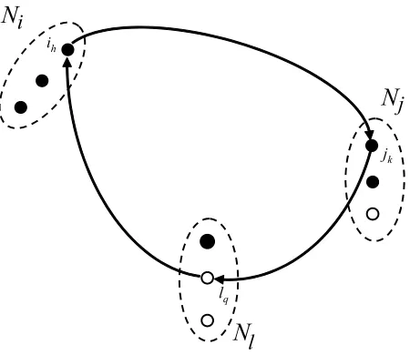
A cyclic exchange corresponds to a directed cycle on the improvement graph as depicted in Figure 4.
Each arc (ih, jk) is associated to a weight, equal to the variation of the
objective function value induced by the corresponding move. The purpose is to represent a feasible group of moves as a cycle in the auxiliary graph, in such a way that the total weight of the arcs of the cycle is equal to the total effect of the group of moves. However, if two or more moves of a cyclic exchange involve the same mode, the overall variation of the objective function is not always equal to the total weight of the cycle, because the effect of the moves could be nonadditive. To overcome this drawback, we only admit cyclic exchanges which affect any mode at most once.
Also note that any feasible cycle with two or more unlabelled node can be splitted in a number of independent cycles equal to the number of unlabelled nodes. If the overall cycle has positive weight, at least one of the component subcycles also has positive weight, and provides an improving move. This allows the following remark.
i
j
l i
h
j
k
l
q N
N
[image:12.595.195.420.126.321.2]N
Figure 4: Graphical representation of the basic local search procedure. The picture displays three subsets of nodes, one for each site (i,jandlrespectively). Siteihosts three facilities, one of which, denoted asih, is of modemh.
Move evaluation To compute the best cyclic exchange, i.e., the one of
max-imum weight, we perform an exhaustive breadth-first generation of all paths of graphG. We first consider all the paths composed of one single arc, then all the paths composed of two arcs and so on. Each path is extended by appending to the end node each outgoing arc, respecting the limitation that all nodes should have different labels and at most one node should be unlabelled. For each path generated, the algorithm evaluates the cost of the cycle obtained by going back from the end of the path to its starting node. This algorithm has computational complexity in O nlmax, where n is the number of nodes of the improvement
graph andlmax the maximum number of nodes in a cycle. The limitation on
the labels of the nodes imposes a bound on the number of nodes in the feasible cycles.
Remark 4 The maximum number of nodes in any cycle is bounded above by
|M|+ 1, i.e.,lmax≤ |M|+ 1.
The efficiency of the neighborhood exploration is strongly improved by the following remark, proved in [1].
Remark 5 Any cycle of positive total weight has at least one starting node such that all the subpaths along the cycle which originate from that node have positive weights.
cycle, there is an alternative path of positive weight which allows to identify the cycle.
4
Computational Experience
In this section we present the computational results of the proposed algorithm, which has been coded in C++, compiled by gcc 4.4.3 and run on a PC equipped with an Intel Core2 Quad-core 2.66 GHz and 4 GB of RAM.
4.1
Benchmark instances
We have considered two benchmark sets of random instances, denoted assquare
and rectangular, respectively. The square instances represent the situation in which a facility can be located in each customer point. The number of columns |J| is therefore equal to the number of rows |I|, and in our benchmark both are set to 1 000. The rectangular instances model the situation in which the distribution of the candidate facility sites is denser than that of the demand centers. The number of columns per mode is therefore larger than the number of rows, and more specifically they are set to 500 rows and 5 000 columns.
In addition to the number of rows and columns, each instance is characterized by the following parameters: the number of modes (|M|), the maximum number of modes for each column (bj), the number of columns used in each mode (Km),
the range of the weights (w), the covering pattern of each column. As for the number of modes, we generated instances with|M| = 2 modes and instances with|M|= 3 modes. The former havebj= 1 for allj ∈J, whereas for the latter
we generated tighter instances withbj = 1, and looser ones with bj = 2. The
number of columns for each mode,Km, is extracted at random, with a uniform
distribution in [0.02|J|; 0.03|J|] for the square instances, in [0.08|J|; 0.10|J|] for the rectangular ones. These values were chosen so as to avoid both the trivial instances in which the optimal solution covers all rows and the easy ones in which the columns are so few that a greedy choice directly provides the optimal result. Theunweighted instances have all weights equal to one, while the weighted instances have random integer weights uniformly distributed in {1, . . . ,10}. Finally, the covering pattern can be uniform, i. e. each column covers the same rows in all modes, or assorted, i. e. the covered rows are selected independently for each mode. For each combination of the parameters listed above, we have generated a pool of 5 instances: the set of rows covered by each column is generated at random with a uniform distribution, imposing a 5% density1. In order to avoid easy instances, we imposed that each column
should cover at least one row in each mode and that each row should be covered by at least two columns in each mode.
Overall, we generated 60 instances for each of the two benchmark sets.
4.2
Parameter tuning
A first computational campaign has been devoted to tuning the parametersthat controls the shaking mechanism of theVNS procedure, the criterium to select the incumbent solution from the neighborhood, and the size of the neighborhood itself.
First, remark that the number of columnsKmused in each modem∈M is
given by the problem instance. Since the shaking procedure replacessof these columns withsunused ones in each mode, necessarilys≤min (Km,|J| −Km).
In our experiments we always set s ≤ Kmin = minm∈MKm because in our
benchmarks Km < |J| −Km for all m ∈ M. We considered three different
ranges for parameters:
• [smin;smax] = [5;Kmin];
• [smin;smax] = [5;Kmin/2];
• [smin;smax] = [Kmin/2;Kmin]
The first tuning leaves the parameter completely free to evolve depending on the results of the search. The second one avoids the larger values, thus reducing the diversification effect of shaking. The third one, by contrast, stresses the effect of diversification. We did not consider values ofssmaller than 5 because preliminary experiments showed that, most of the time, a search starting very close to the best known solution ends up again in it, with a useless waste of computational time.
As for the exploration of the neighborhood, we considered two common variants: the global-best strategy explores the whole neighborhood, returning the best solution found; thefirst-best strategy terminates the search as soon as an improving solution is found. In a single iteration, of course, the first strategy yields a stronger improvement, but the latter allows to perform more iterations in the same time. Experimental evidence suggests that in different problems either strategy can perform better [9].
Global-best First-best
s Gap BK itot i∗ Gap BK itot i∗
[5;Kmin] 0.25% 607.93 162.98 0.40% 872.08 166.70
5;Kmin 2
0.19% 609.03 270.87 0.40% 871.83 166.70
Kmin
2 ;Kmin
0.56% 603.10 64.13 0.59% 871.18 12.27
Table 1: Computational results of the parameter tuning phase on the square instances
Global-best First-best
s Gap BK itot i∗ Gap BK itot i∗
[5;Kmin] 0.09% 370.28 192.05 0.15% 425.87 169.88
5;Kmin 2
0.09% 370.37 194.70 0.15% 426.07 169.88
K
min
2 ;Kmin
[image:15.595.139.473.124.213.2]
0.22% 356.38 3.02 0.22% 427.70 6.40
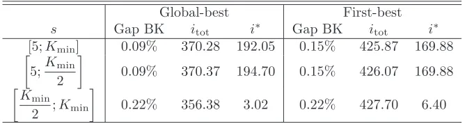
Table 2: Computational results of the parameter tuning phase on the rectangu-lar instances
of the two neighborhood exploration strategies, Table 1 reports the average values computed on all the square instances of the following statisics: column “Gap BK” provides the average percentage gap (z∗−z)/zbetween the result
z obtained by the current parameter setting and the best result z∗ found in
the overall experimental campaign. This is assumed as a reference because the optimal value for these problems is unknown and, as we shall discuss in the following, even a state-of-the-art general purpose solver such as CPLEX 12 is unable to provide meaningful upper bounds on the optimum. Statistics itot andi∗ are the number of local search iterations performed in 600 seconds
and the iteration at which the result z has been found, respectively. Table 2 reports the corresponding information for the rectangular instances. The two tables suggest a clear dominance of the global-best strategy on the first-best strategy: the latter, in fact, has worse results, on average; it finds them earlier, but is unable to improve them, even though it performs more iterations in the same time. The difference between the average performances is confirmed by the application ofWilcoxon’s matched-pairs signed-ranks test[40] to the instance-by-instance results. This test estimates that the probability to obtain such results with a random fluctuation isp= 1.585·10−14
. As for the shaking parameter, the setting which favors diversification over intensification by adopting large values ofsis outperformed by the other two settings (p <10−26
in both cases). The intensifying setting, which restrictss in [5;Kmax/2], proves the better of
the remaining two, with a probability of random fluctuations equal to p = 1.221·10−4
. The intensifying setting has a particularly strong dominance on the square instances, whereas for several rectangular instances the two settings are equivalent. This is partly due to the fact that the two settings behave exactly in the same way as long as the shaking parametershas not yet reached the threshold valuesmax. Since in the allotted time the algorithm performs less
Polynomial vs exponential sized neighborhood
The parameter tuning computational campaign described above has been car-ried out on theVNSimplementing the exponentially large neighborhood (VLNS). Indeed, experiments on the polynomial-size neighborhood confirm the perfor-mance with respect to the shaking parameter and the exploration strategy: the intensifying setting and the globbest exploration strategy outperform the al-ternative settings. The results are, however, worse than those obtained, in the same time, by theVLNS procedure. In particular, the average gap with respect to the best known result is 0.24% for the square instances and 0.12% for the rectangular ones, versus 0.19% and 0.09% (see Tables 1 and 2). Considering instance-by-instance solutions, Wilcoxon’s test estimates the probability to ob-tain such a difference with a random fluctuation to bep= 1.011·10−12
when considering all six parameter settings, and p = 4.058·10−12
when consider-ing only the best one. Usconsider-ing a good parameter settconsider-ing probably allows to find optimal or nearly optimal solutions even exploring a smaller neighborhood.
An interesting remark is that, when applying the first-best exploration strat-egy, the difference between the polynomial and exponential size neighborhoods is less marked (0.44% and 0.16% versus 0.40% and 0.15% for square and rectangu-lar instances, respectively). This is easily explained by the fact that the first-best strategy terminates the exploration of the neighborhood as soon as an improv-ing solution has been found and that the moves adopted in the polynomial-size neighborhood correspond, in the improvement graph, to cycles of two arcs vis-iting an unlabelled node. These cycles are among the first explored in the exponential-size neighborhood. Therefore, theVLNS procedure with the first-best exploration strategy has a good probability to return a solution included also in the polynomial-size neighborhood. Anyway, this remark does not in-volve the best performing parameter setting. Our conclusion is that, even if the polynomial-size neighborhood can be explored more quickly, the exponential-size one provides solutions of better quality and a stronger robustness with respect to local optima. On the basis of such results, in the following experiments we have adopted the intensifying setting for the shaking parameter, the global-best exploration strategy and the exponential-size neighborhood.
4.3
Performance of the different phases of the algorithm
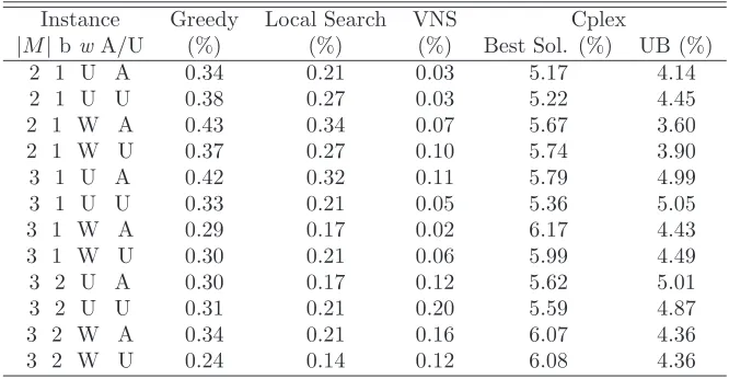
include the greedy and local search phases. Finally, CPLEX runs for 1 hour. Tables 3 and 4 refer, respectively, to the square and rectangular instances. The first column (Instance) provides a description of each subclass of instances: |M| is the number of modes,bthe capacity of each location – that, we recall, has the same value for allj∈J –;wdistinguishes the weighted instances (W) from the unweighted one (U); A/U distinguishes the assorted mode instances, denoted withA, from the uniform mode instances, denoted withU. The following three columns report the percentage gap between the result obtained by each phase of the algorithm and the best known one. Finally, the last two columns provide the percentage gap between the heuristic solution returned by CPLEX and the best known one, and the percentage gap between the upper bound computed by CPLEX and the best known result ((U B−z∗)/z∗). The value in each row
is the average over the 5 instances of each group.
Instance Greedy Local Search VNS Cplex
|M|bwA/U (%) (%) (%) Best Sol. (%) UB (%)
2 1 U A 0.85 0.75 0.12 15.21 15.68
2 1 U U 0.78 0.65 0.10 14.82 11.08
2 1 W A 1.03 0.81 0.15 16.03 13.38
2 1 W U 0.85 0.66 0.20 17.48 8.85
3 1 U A 0.85 0.68 0.24 19.38 14.58
3 1 U U 0.63 0.44 0.07 15.23 12.48
3 1 W A 0.99 0.73 0.12 14.82 12.55
3 1 W U 0.66 0.59 0.10 12.93 10.40
3 2 U A 0.51 0.37 0.16 19.51 14.68
3 2 U U 0.69 0.45 0.45 17.57 12.14
3 2 W A 0.68 0.50 0.28 21.03 12.74
3 2 W U 0.71 0.40 0.30 17.68 9.93
Table 3: Average gap (with respect to the best known solution) computed on each group of square instances.
The greedy algorithm finds in a fraction of a second a solution very close to the best known one (on average 0.55% worse). The local search procedure improves it in few seconds, reducing the average gap to 0.41%. Finally, theVNS
algorithm further improves the solution reducing the gap to 0.14% on average. By contrast, CPLEX after one hour returns a heuristic solution which is on average 11% worse than the best known one. This suggests that an ad hoc
Instance Greedy Local Search VNS Cplex
|M|bwA/U (%) (%) (%) Best Sol. (%) UB (%)
2 1 U A 0.34 0.21 0.03 5.17 4.14
2 1 U U 0.38 0.27 0.03 5.22 4.45
2 1 W A 0.43 0.34 0.07 5.67 3.60
2 1 W U 0.37 0.27 0.10 5.74 3.90
3 1 U A 0.42 0.32 0.11 5.79 4.99
3 1 U U 0.33 0.21 0.05 5.36 5.05
3 1 W A 0.29 0.17 0.02 6.17 4.43
3 1 W U 0.30 0.21 0.06 5.99 4.49
3 2 U A 0.30 0.17 0.12 5.62 5.01
3 2 U U 0.31 0.21 0.20 5.59 4.87
3 2 W A 0.34 0.21 0.16 6.07 4.36
[image:18.595.139.472.124.297.2]3 2 W U 0.24 0.14 0.12 6.08 4.36
Table 4: Average gap (with respect to the best known solution) computed on each group of rectangular instances.
The hardness of the MM-LCP for MIP solvers is confirmed by the scarce quality of the upper bound provided. In fact, the gap with respect to the upper bound is on average 8%. Indeed, this bound is often equal to the trivial combinatorial bound given by the sum of the weights of all rows in all modes, which can be computed in negligible time. This happens for all rectangular instances and for more than half of the square instances.
4.4
Comparison with heuristic concentration
To evaluate the performances of the proposed VNS approach, we have also implemented an alternative heuristic, based on theHeuristic Concentration ap-proach, which has been applied to the MCLP in [36] and, to the best of our knowledge, is the most effective heuristic to solve large instances of this problem. This is a two-stage metaheuristic. In the first stage, q random starting solutions are improved by a basic local search heuristic, and all thexjmvariables
which are set to 1 in the bestt ≤ q local optimal solutions are collected in a list, called the concentration set (CS). In the second stage, Formulation (1) is solved with CPLEX 12.0, under the additional constraint that all variables not belonging to the CS are set to zero. The CS, in fact, is considered likely to contain the optimal solution, provided that the basic heuristic is good, and the number of restarts q and of best solutions t are large enough. On the other hand, excessively large values ofq increase the computational time of the first stage and excessively large values of t increase the computational time of the second stage.
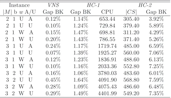
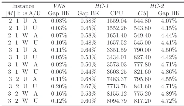
compare theVNSapproach with the best parameter setting, the first stage of the
HC algorithm (columnHC-1), and the final result returned by the second stage of the HC algorithm (column HC-2). The former table refers to the square instances, the latter to the rectangular ones. The first column of each table identifies each subclass of instances, and each row reports the average results over the 5 instances of the subclass. The second column provides the gap with respect to the best known result achieved by theVNS approach with the best parameter setting as identified above. The following two columns provide the corresponding gap and the computational time in seconds for theq= 30 random restarts of the first stage ofHC . The last two columns provide the number of binary variables xjm which compose the CS and the percentage gap for the
result returned by the second stage of the HC algorithm with a time limit of 1 800 seconds.
Instance VNS HC-1 HC-2
[image:19.595.157.457.299.472.2]|M|bwA/U Gap BK Gap BK CPU |CS| Gap BK 2 1 U A 0.12% 1.14% 653.44 305.40 3.92% 2 1 U U 0.10% 1.24% 729.84 379.40 5.89% 2 1 W A 0.15% 1.47% 698.81 311.20 4.29% 2 1 W U 0.20% 1.43% 786.55 371.40 5.26% 3 1 U A 0.24% 1.17% 1719.74 485.00 6.59% 3 1 U U 0.07% 1.39% 1925.27 560.00 7.06% 3 1 W A 0.12% 1.23% 1836.91 488.60 6.13% 3 1 W U 0.10% 1.16% 2033.36 552.80 7.25% 3 2 U A 0.16% 1.06% 3780.03 483.60 6.01% 3 2 U U 0.45% 1.64% 4091.90 568.80 7.59% 3 2 W A 0.28% 1.09% 4075.43 486.60 6.48% 3 2 W U 0.29% 1.49% 4401.99 549.20 7.35%
Table 5: Computational results of the HC algorithm on the square instances.
The results show that, contrary to what happens for the basicMLCP, the
Instance VNS HC-1 HC-2
[image:20.595.153.456.123.297.2]|M|bwA/U Gap BK Gap BK CPU |CS| Gap BK 2 1 U A 0.03% 0.58% 1559.04 544.80 4.07% 2 1 U U 0.03% 0.45% 1552.26 543.80 4.15% 2 1 W A 0.07% 0.58% 1651.40 549.40 4.44% 2 1 W U 0.10% 0.48% 1657.52 545.00 4.41% 3 1 U A 0.11% 0.64% 3351.59 790.00 4.50% 3 1 U U 0.05% 0.53% 3434.01 827.40 4.42% 3 1 W A 0.02% 0.50% 3573.03 777.80 4.71% 3 1 W U 0.06% 0.44% 3603.25 821.60 4.86% 3 2 U A 0.11% 0.68% 7483.37 795.60 4.55% 3 2 U U 0.20% 0.67% 7713.76 841.60 4.71% 3 2 W A 0.16% 0.53% 8155.12 775.20 4.89% 3 2 W U 0.12% 0.60% 8094.79 817.20 4.72%
Table 6: Computational results of the HC algorithm on the rectangular in-stances.
percentage gap obtained byHC is much better than that obtained by CPLEX on the whole problem (see Tables 3 and 4), the experiments do not support the effectiveness ofHC on theMM-LCP.
It could be objected that the bad performance of HC could be due to an excessive value of the two crucial parametersq and t. This idea, however, is contradicted by the number of variables which compose theMIP problem used in the second stage of theHC algorithm. As it can be seen from column|CS| in Tables 5 and 6, the number of binary variables is strongly reduced by the heuristic selection performed in the first phase. For the square instances, in fact, the binary variablesxdecrease from 2 000−3 000 (depending on the number of modes) to around 300−500, while the number of variables which must be set to 1 isP
m∈MKm∈[50; 75]. For the rectangular instances, the binary variablesx
decrease from 10 000−15 000 to around 500−800 andP
m∈MKm∈[100; 150].
5
Conclusion
In this paper, we study theMultimode Covering Location Problem (MM-CLP), which is a generalization of the Maximal Covering Location Problem (MCLP). This problem consists of locating a given number of facilities of different types to serve demand centers with the restriction that only a limited number of different types can be activated in each candidate facility site.
is confirmed by the poor quality of the upper bound that they are able to compute. Indeed, for most of our benchmark instances, this bound is often equal to the trivial combinatorial bound given by the sum of the weights of all rows in all modes. Nevertheless, the problem admits a constant factor approximation guarantee that we proved by means of two greedy algorithms extending in a nontrivial way a similar property of theMCLP.
To improve the greedy solutions, we have developed aVNS approach, which implements aVLSNS algorithm as its basic local search procedure. The pro-posed procedure is able to compute good quality solutions in short computa-tional times. The viability of the proposed approach is also corroborated by a comparison with an alternativeVNS based on a polynomial-size neighborhood and aHeuristic Concentrationalgorithm, which is, to the best of our knowledge, the most effective approach to solve large instances of theMCLP.
References
[1] R.K. Ahuja, J.B. Orlin, D. Sharma (2003) A composite very large-scale neighborhoodstructure for the capacitated minimum spanning tree problem
Operations Research Letters, 31, pp. 185–194
[2] S. Arora, N. Gupta, S. Khuller, Y. Sabharwal, S. Singhal (2014) Facility location with redblue demands Operations Research Letters, 42, pp. 462– 465
[3] D. Beltr´an-Cano, B. Meli´an-Batista, J. M. Moreno-Vega (2009) Solving the Rectangle Packing Problem by an iterative hybrid heuristicLecture Notes in Computer Science, Volume 5717, pp. 673–680
[4] P. Berman, B. DasGupta, E. Sontag (2007) Randomized approximation algorithms for set multicover problems with applications to reverse engi-neering of protein and gene network. Discrete Applied Mathematics, 155 (6-7), pp. 733–749.
[5] O. Berman, Z. Drezner, D. Krass (2010) Generalized coverage: New de-velopments in covering location models.Computers & Operations Research
37, pp. 1675–1687
[6] K. Bicakci, I. E. Bagci, B. Tavli, Z. Pala (2013) Neighbor Sensor Networks: Increasing Lifetime and Eliminating Partitioning Through Cooperation.
Computer Standards & Interfaces, 35 (4), pp 396–402.
[7] C.H. Chung, Recent applications of the Maximal Covering Location Prob-lem (MCLP) model,Journal of the Operational Research Society37 (1986) 735-746.
[8] R.L. Church, C.S. ReVelle (1974) The maximal covering location problem.
[9] F. Colombo, R. Cordone, G. Lulli (2013) A Variable Neighborhood Search Algorithm for the Multimode Set Covering Problem.Journal of Global Op-timization, [in press: DOI 10.1007/s10898-013-0094-6]
[10] T. H. Cormen, C. E. Leiserson, R. L. Rivest, C. Stein (2001)Introduction to algorithms. MIT Press.
[11] R. Aringhieri, R. Cordone, (2011) Comparing local search metaheuristics for the Maximum Diversity Problem,Journal of the Operational Research Society, 62 (2), pp. 266–280
[12] R. Cordone, G. Lulli (2013) A GRASP metaheuristic for microarray data analysis Computers & Operations Research, 40 (12), pp. 3108–3120
[13] J. Current, M. O’Kelly (1992) Locating emergency warning sirens,Decision Sciences 23, pp. 221–234.
[14] M.S. Daskin, P.C. Jones, T.J. Lowe (1990) Rationalizing tool selection in a flexible manufacturing system for sheet metal products, Operations Research38, pp.1104–1115.
[15] M.S. Daskin (1995) Network and discrete location: Models, algorithms, and applications. J. Wiley and Sons, Inc., New York.
[16] P. Dell’Olmo, N. Ricciardi, A. Sgalambro (2014) Multiperiod Maximal Cov-ering Location Model for the optimal location of intersection safety cameras on an urban traffic network.Working Paper.
[17] B.T. Downs, J.D. Camm (1996) An exact algorithm for the maximal cover-ing location problem,Naval Research Logistics Quarterly 43, pp. 435–461.
[18] F.R. Dwyer, J.R. Evans (1981) A branch and bound algorithm for the list selection problem in direct mail advertising, Management Science 27, pp. 658–667.
[19] D. Eaton, M. Hector, V. Sanchez, R. Latingua, J. Morgan (1986) Determin-ing ambulance deployment in Santo DomDetermin-ingo, Dominican RepublicJournal of the Operational Research Society, 37, pp. 113–126.
[20] H.A. Eiselt, C.L. Sandblom (2004) Decision Analysis, Location Models, and Scheduling Problems. Springer-Verlag, BerlinHeidelbergNew York.
[21] T. A. Feo, M. G. C. Resende (1989) A probabilistic heuristic for a com-putationally difficult set covering problemOperations Research Letters, 8, pp. 67–71.
[23] R. D. Galvao, C. ReVelle (1996) A Lagrangean heuristic for the maximal covering location problem. European Journal of Operational Research 88, pp. 114–123.
[24] M. R. Garey, D. S. Johnson (1979)Computers and Intractability: A Guide to the Theory of NP-completeness. W. H. Freeman and Company, New York.
[25] G. Ghiani, F. Guerriero, R. Musmanno (2002) The capacitated plant loca-tion problem with multiple facilities in the same site.Computers & Oper-ations Research29, pp. 1903–1912
[26] P. Hansen, N. Mladenovi¸c, J. A. Moreno P´erez (2010) Variable Neighbour-hood Search: Methods and Applications. Annals of Operations Research, 175, pp. 367–407.
[27] M. I. Hosny, C. L. Mumford (2010) Solving the One-commodity Pickup and Delivery Problem using an adaptive hybrid VNS/SA approach.Lecture Notes in Computer Science, Volume 6239, pp. 189–198
[28] E.S. Hougland, N.T. Stephens (1976) Air pollutant monitor siting by ana-lytical techniques,Journal of the Air Pollution Control Association26, pp. 52–53.
[29] L.A.N. Lorena, M.A. Pereira (2002) A lagrangean/surrogate heuristic for the maximal covering location problem using Hillsman’s edition. Interna-tional Journal of Industrial Engineering, 9 (1), pp. 57–67.
[30] M.T. Melo, S. Nickel, F. Saldanha-da-Gama (2009) Facility location and supply chain management – A review, European Journal of Operational Research196, pp. 401–412
[31] P. B. Mirchandani, R.L. Francis (Eds.) (1990) Discrete location theory. Wiley-Interscience.
[32] J.T. Pastor (1994) Bicriterion programs and managerial locations: Appli-cation to the banking sector,Journal of the Operational Research Society
45, pp. 1351–1362.
[33] M.A. Pereira, L.A.N. Lorena, E.L.F. Senne (2007) A column generation approach for the maximal covering location problem. Intl. Transaction in Operations Research 14, pp. 349–364
[34] H.K. Rajagopalan, C. Saydam, L. Xiao (2008) A multiperiod set covering location model for dynamic redeployment of ambulances. Computers & Operations Research, 35, pp. 814–826.
[36] C. ReVelle, M. Scholssberg, J. Williams (2008) Solving the maximal cover-ing location problem with heuristic concentration.Computers & Operations Research35, pp. 427–435
[37] C.S. ReVelle, H.A. Eiselt (2005) Location analysis: A synthesis and survey.
European Journal of Operational Research165, pp. 1–19.
[38] P.M. Thompson, J.B. Orlin (1989) The theory of cyclic transfers,Working Paper OR200-89, Operations Research Center, MIT, Cambridge, MA.
[39] R.V. Vohra, N. Hall (1993) A probabilistic analysis of the maximal covering location problemDiscrete Applied Mathematics, 43, pp. 175–183.