Cassini observations of ionospheric plasma in
1
Saturn’s magnetotail lobes
2
M. Felici,1,2,3 C.S. Arridge,3 A.J. Coates,1,2 S.V. Badman,3 M.K. Dougherty,4
C.M. Jackman,5 W.S. Kurth,6 H. Melin,7 D.G. Mitchell,8 D.B. Reisenfeld,9
and N. Sergis,10
Corresponding author: M. Felici, Mullard Space Science Laboratory, University College
Lon-don, Holmbury St. Mary, Dorking, Surrey, RH5 6NT, UK. (marianna.felici.12@ucl.ac.uk)
Abstract. Studies of Saturn’s magnetosphere with the Cassini mission
3
have established the importance of Enceladus as the dominant mass source
4
for Saturn’s magnetosphere. It is well known that the ionosphere is an
im-5
portant mass source at Earth during periods of intense geomagnetic
activ-6
ity, but lesser attention has been dedicated to study the ionospheric mass
7
source at Saturn. In this paper we describe a case study of data from
Sat-8
urn’s magnetotail, when Cassini was located at ≃ 2200 hours Saturn local
9
time at 36 RS from Saturn. During several entries into the magnetotail lobe,
10
tailward-flowing cold electrons and a cold ion beam were observed directly
11
adjacent to the plasma sheet and extending deeper into the lobe. The
elec-12
trons and ions appear to be dispersed, dropping to lower energies with time.
13
The composition of both the plasma sheet and lobe ions show very low fluxes
14
(sometimes zero within measurement error) of water group ions.
15
The magnetic field has a swept-forward configuration which is atypical for
16
this region and the total magnetic field strength is larger than expected at
17
this distance from the planet. Ultraviolet auroral observations show a dawn
18
brightening and upstream heliospheric models suggest that the magnetosphere
19
is being compressed by a region of high solar wind ram pressure. We
inter-20
pret this event as the observation of ionospheric outflow in Saturn’s
mag-21
netotail. We estimate a number flux between (2.95±0.43)×109 and (1.43±
22
0.21)×1010 cm−2s−1, one or about two orders magnitude larger than
sug-23
gested by steady state MHD models, with a mass source between 1.4 ×10²
24
and 1.1 ×10³ kg/s. After considering several configurations for the active
at-25
mospheric regions, we consider as most probable the main auroral oval, with
26
associated mass source between 49.7±13.4 and 239.8±64.8 kg/s for an
av-27
erage auroral oval, and 10±4 and 49±23 kg/s for the specific auroral oval
28
morphology found during this event. It is not clear how much of this mass
29
is trapped within the magnetosphere and how much is lost to the solar wind.
30
1. Introduction
Saturn’s magnetosphere is a complex multi-component plasma system with several
inter-31
nal plasma sources in addition to the solar wind. The largest internal plasma source is from
32
photoionisation and electron-impact ionisation of neutral water and nitrogen molecules
33
from the icy moon Enceladus. These ions are subsequently processed by photolytic and
34
radiolytic processes to produce H+, and a variety of water group ions such as OH+ and
35
O+ that are collectively referred to as W+. The other natural satellites, the rings, and
36
Saturn’s atmosphere are minor internal sources. The solar wind also plays a role as an
37
external plasma source. A number of studies have focused on the moons, rings and solar
38
wind as plasma sources, to constrain the extent to which they drive the system. In this
39
paper we provide the first in situ constraints on the role that the ionosphere plays as a
40
mass source for Saturn’s magnetotail, via the first observation of ionospheric outflow at a
41
giant planet.
42
1.1. Plasma sources and transport in Saturn’s magnetosphere
Shemansky et al. [1993] presented Hubble Space Telescope (HST) observations of an
43
OH torus extending from 3 to 8 RS (1RS = 60268 km). They identified Enceladus, and
44
to a lesser extent the other icy moons, as H2O sources for the magnetosphere. Jurac et al.
45
[2002] andRichardson and Jurac [2004] estimated the amount of H2O needed to maintain
46
the OH cloud and found that a source rate of 3.75×1027 H
2O molecules/s (112 kg/s)
47
was required to maintain this cloud, of which 93 kg/s must be coming from the orbit of
48
Enceladus. This estimate sits within a range of estimated rates between 1026 and 1028
49
molecules/s (≃35-350 kg/s) [Tokar et al., 2006; Waite et al., 2006; Hansen et al., 2006].
50
The large variability in these figures may be a natural result of the time-variability of the
51
Enceladus source. Following processing of these neutrals by neutral-plasma chemistry, the
52
total plasma source rate is around 60-100 kg/s [Fleshman et al., 2013].
53
Titan has also been studied as a source of mass for Saturn’s magnetosphere. Johnson
54
et al. [2009] estimates a total ion loss rate from Titan of 1−5×1026 amu/s (0.16-0.83
55
kg/s). Coates et al. [2012] estimated a loss rates of (8.9, 1.6, 4.0) ×1025 amu/s for three
56
crossings of Titan’s tail, for an average loss rate of 0.8 kg/s.
57
Saturn’s main rings have an O+ and O+
2 atmosphere which can be ionised and act as
58
a mass source for the magnetosphere [Tokar et al., 2005; Johnson et al., 2006a; Johnson
59
et al., 2006b; Bouhram et al., 2006; Luhmann et al., 2005; Martens et al., 2008; Tseng 60
et al., 2010]. The ring atmosphere was predicted to vary seasonally as the incidence angle
61
of the solar radiation on the main rings varies seasonally [Tseng et al., 2010]. Using a
62
photochemical model and Cassini plasma spectrometer (CAPS) data, Elrod et al. [2012]
63
demonstrated that observed changes in the ring plasma over time were due to seasonal
64
change in the production of neutrals from Saturn’s ring atmosphere. We are not aware of
65
any published estimates of the mass loading rate due to the rings.
66
Plasma produced in the inner magnetosphere from these sources is transported to the
67
outer magnetosphere. This transport is regulated by the centrifugally driven interchange
68
instability [Mauk et al., 2009, and references therein]. The most detectable signature of
69
this process is the injection of hot plasma into the inner magnetosphere accompanied by
70
magnetic pressure enhancements or deficits [e.g.Hill et al., 2005;Andr´e et al., 2005, 2007;
71
Thomsen, 2013].
72
The solar wind and ionosphere are thought to be secondary sources but the source
73
rates have only been estimated and there are no observational constraints. To estimate
74
the magnitude of the solar wind source a common approach is to multiply the solar
75
wind mass flux nSWvSW by the cross-sectional area of the magnetosphere to obtain an
76
upper limit for the source rate: nSWvSWπR20. An efficiency factor O(10−3) is included
77
to account for diversion of the the solar wind and magnetosheath plasma around the
78
magnetosphere and the ability of magnetosheath plasma adjacent to the magnetopause
79
to enter the magnetosphere [Hill, 1979; Hill et al., 1983; Vasyliu˜nas, 2008; Bagenal and
80
Delamere, 2011]. Applying this logic with a solar wind number density between 0.002
81
and 0.4 cm3, and a solar wind speed between 400 and 600 km/s [Crary et al., 2005]
82
with a magnetopause of cross-sectional area π(30 RS)2 (using the terminator radius of
83
the magnetopause from Kanani et al.[2010]), gives an upper limit of between 8.21×1027
84
and 2.46×1030 protons/s (hence between about 13 and 4119 kg/s). Combined with the
85
efficiency factor of 10−3 the solar wind is a minor source.
86
1.2. Ionospheric outflow from Saturn’s atmosphere
The physical mechanisms which lead to the ionosphere outflowing into space were
the-87
orised before the ionospheric outflow was detected at Earth. Dessler and Michel [1966]
88
andBauer [1962] argued that, since the magnetospheric tail has a lower pressure than the
89
ionosphere, there should be a continuous escape of thermal plasma from the ionosphere
90
into the tail (referred to just H+ and He+ at Earth). By analogy with the solar wind,
91
Axford [1968] suggested that this flow should be supersonic and named it the polar wind.
92
The classical polar wind is an ambipolar outflow of thermal plasma from the high
lati-93
tude ionosphere. The faster upflowing electrons create a charge separation with the more
94
gravitationally-bound ions, generating an ambipolar electric field that accelerates the ions
95
to achieve charge neutrality. The plasma, travelling and then escaping the topside of the
96
ionosphere, undergoes four transitions: from chemical to diffusion dominance, from being
97
subsonic to supersonic, from a collision dominated to a collionsless regime, a transition
98
from heavy to light ions (at Earth O+ and H+) since the light ions are less gravitationally
99
bound.
100
A steady state polar wind outflow is highly improbable. Magnetospheric electric fields
101
make the ionosphere-polar wind system convect constantly across the polar region, polar
102
cap, nightside auroral oval, nighttime trough, and sunlit hemisphere. When the
mag-103
netic activity increases, plasma convection speeds and particle precipitations intensify.
104
Three-dimensional time-dependent simulations of the global ionosphere and polar wind
105
have shown that, when the geomagnetic activity changes, the temporal variations and
106
horizontal plasma convection affect the polar wind and its dynamics. Three-dimensional
107
models (a global ionosphere-polar wind model) studied how much a geomagnetic storm
108
(for different solar cycles conditions) would have influenced the atmospheric system [
Gan-109
guli, 1996; Schunk and Nagy, 2009, and references therein]. Polar wind outflow increases
110
with geomagnetic activity.
111
Different mathematical approaches have been used over the years to model the
complex-112
ity of the polar wind, such as hydrodynamical and hydromagnetic modelling, generalized
113
transport, and kinetic models. Also, numerous studies have been conducted of the
non-114
classical polar wind, which may contain, for example, ion beams or hot electrons. A
115
wealth of processes might be acting in the polar wind and still understanding is needed
116
[Ganguli, 1996].
117
Observational evidence of the polar wind at Earth was presented by Hoffman [1970]
118
using data from Explorer 31 showing field-aligned aligned H+ with speed≃10 km/s, and
119
flux ≃108 cm−2s−1 above 2500 km altitude. Using ISIS 2 and OGO data, similar results
120
for H+were obtained, plus O+and He+observations were added to the picture byBrinton
121
et al. [1971]; Taylor and Walsh [1972]; Hoffman et al. [1974]; Taylor Jr. and Cordier 122
[1974]; Hoffman and Dodson [1980]. More recently, Chandler et al. [1991] measured ion
123
density, velocity and flux variations of polar wind outflows using DE 1 data.
124
Electron temperature anisotropies, the relationship between the plasma pressure
gradi-125
ent between the ionosphere and deep magnetosphere, and the process of ambipolar
diffu-126
sion along magnetic field lines was established using Akebono data [Abe et al., 1993a, b;
127
Yau et al., 1995]. Observations of ionospheric outflow in the magnetosphere are harder
128
to make given the temperature of the plasma and charging of the spacecraft. Using
Clus-129
ter data, Engwall et al. [2009a] and Engwall et al. [2009b] inferred a total outflow from
130
Earth’s polar ionosphere of the order of 1026 ions/s, which confirmed previous simulation
131
results arguing for the continuous presence of a low-energy ion population in the lobes. In
132
addition, they inferred that the solar wind dynamic pressure and interplanetary magnetic
133
field played a role in influencing these populations in the lobes.
134
The polar wind is an important source of plasma in Earth’s magnetosphere during
135
periods of geomagnetic activity. The extent of the ionosphere as a plasma source at
136
Saturn has been investigated using numerical models [Frey, 1997; Glocer et al., 2007].
137
These models solve the field-aligned gyrotropic transport equation [Gombosi and Nagy,
138
1989] for ions and electrons and simulate multiple convecting field line solutions.
139
Glocer et al.[2007] applied this model to Saturn, adapting the chemistry for the
compo-140
sition of Saturn’s thermosphere. The model considers the behavior of H+ and H+
3. It
as-141
sumes a stationary neutral atmosphere and models a range in altitude from 1400 (chemical
142
and thermal equilibrium) to 61000 (lower pressure) km. The background neutral
atmo-143
sphere required as an input relies on analysis of the stellar occultation measurements (low
144
latitude) of the Voyager 2 Saturn flyby, presented by Smith et al. [1983]. The estimates
145
for temperature and density of the neutrals were made at low latitudes, therefore the
146
model counts for the uncertainty on these parameters with a wide array of temperatures
147
(420-1500 K) which takes into account the possible density and temperature variations
148
from low to high latitudes. From this model, Glocer et al.[2007] estimate the polar wind
149
number flux of 7.3×10⁶ to 1.7×108 cm−2s−1 at 10000 km, providing a total source rate
150
to the magnetosphere of 2.1×1026 to 7.5×1027 s−1, for a source rate between 0.35 kg/s
151
and 1.25 kg/s.
152
Unfortunately, there are no observational constraints with which to compare these model
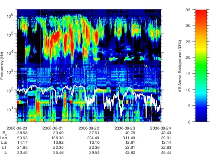
153
results. In this paper we report the detection of cold plasma in Saturn’s magnetotail
154
lobes, consider the interpretation of polar wind outflow, and use these observations to
155
constrain the ionosphere as a source of plasma for Saturn’s magnetosphere. In section 2
156
we describe the instrumentation used for this study, in section 3 we show an overview of the
157
observations, the spacecraft trajectory, and the inferred upstream solar wind conditions.
158
The detailed case study is presented in section 4 and various interpretations discussed in
159
section 5. The implications for the physics of Saturn’s magnetosphere are presented in
160
section 5.
161
2. Intrumentation
We use data from the Cassini Dual Technique Magnetometer (MAG) [Dougherty et al.,
162
2004], the Cassini Plasma Spectrometer (CAPS) [Young et al., 2004], the Magnetospheric
163
Imaging Instrument (MIMI) [Krimigis et al., 2004], the Radio and Plasma Wave Science
164
instrument (RPWS) [Gurnett et al., 2004], and the Ultraviolet Imaging Spectrometer
165
(UVIS) [Esposito et al., 2004].
166
CAPS measures the energy per charge and arrival direction of electrons and ions. The
167
instrument consists of three sensors: the Electron Spectrometer (ELS) which measures
168
electrons from 0.7 eV/q to 29 keV/q, the Ion Beam Spectrometer (IBS) which measures
169
narrow ion beams from 1 eV/q to 50 keV/q, and the Ion Mass Spectrometer (IMS) that
170
measures ions from 1 eV/q to 50 keV/q, followed by a time of flight (TOF) analyzer for the
171
determination of mass per charge of incoming particles. A motor-driven actuator rotates
172
the sensor package to provide 208-degree scanning in the azimuth of the spacecraft, nearly
173
2π sr of the sky can be swept across every 3 minutes; spacecraft rolls can occasionally
174
increase the field of view to 4π sr.
175
MAG measures the strength and direction of the magnetic field around Saturn via a
176
fluxgate magnetometer and a vector helium magnetometer mounted on an 11 m spacecraft
177
boom, with the FGM located in the middle of the boom and the VHM at the end. The
178
magnetometer boom distances the sensors from the stray magnetic field associated with
179
the spacecraft and its subsystems and, especially with spacecraft generated field variations,
180
spacing the sensors at different distances along the boom allows this field to be better
181
characterised and removed from the observations. This study uses data from the fluxgate
182
magnetometer.
183
MIMI consists of three detectors: Charged Energy Mass Spectrometer (CHEMS), the
184
Low Energy Magnetospheric Measurement System (LEMMS), and the Ion and Neutral
185
Camera (INCA). CHEMS measures charge and compositions of ions with energy range
186
between ≃ 3 to 220 keV/q, combining electrostatic deflection and TOF to measure the
187
energy and composition of the energetic particles. INCA operates in two different modes,
188
over the energy range between 7 keV/nuc and 3 MeV/nuc. In its ion mode INCA measures
189
directional distribution, energy spectra and composition of ions and, in its neutral mode, it
190
takes remote images of the global distribution of the energetic neutral atoms, determining
191
their composition and energy spectra for each image pixel. INCA has a field of view of
192
120◦ in latitude and 90◦ in azimuth, whereas when the spacecraft is rotating the camera
193
covers about 4 π sr. LEMMS consists of two oppositely directed telescopes, a low-energy
194
telescope designed to detect ions with energy≥30 keV and electrons with energy between
195
15 keV and 1 MeV, and a high-energy telescope for ions with energy range between 1.5
196
and 160 MeV/nuc and electrons (0.1-5 MeV).
197
The Blackett Laboratory, Imperial College
London, United Kingdom.
5Department of Physics and Astronomy,
University of Southampton, United
Kingdom.
6Department of Physics and Astronomy,
University of Iowa, Iowa, United States of
America.
7Department of Physics and Astronomy,
University of Leicester, United Kingdom.
8Johns Hopkins University Applied
Physics Laboratory, Laurel, Maryland,
United States of America.
9Department of Physics and Astronomy,
University of Montana, Missoula, Montana,
United States of America.
10Office for Space Research, Academy of
RPWS measures radio emissions, plasma waves, thermal plasma and dust in the vicinity
198
of Saturn. Three nearly orthogonal electric field antennas detect electric fields over a
199
frequency range from 1 Hz to 16 MHz, and three orthogonal search coil antennas measure
200
magnetic fields between 1 Hz to 12 kHz. A Langmuir probe is used to measure the
201
electron density and temperature. Five receiver systems process signals from the electric
202
and magnetic antennas.
203
UVIS measures ultraviolet light between the wavelengths of 55.8 and 190 nm for imaging
204
spectroscopy and spectroscopic measurements of the structure and composition of the
205
atmospheres of Titan and Saturn, rings, and surfaces, through two telescopes. It comprises
206
two spectrographic channels: an extreme ultraviolet channel (EUV), that measures spectra
207
between 55.8 and 118 nm, and a far ultraviolet channel (FUV), which measures spectra
208
between 110 and 190 nm.
209
3. Overview and upstream conditions
Figure 1 shows Cassini’s trajectory on our day of interest, 21 August 2006 (day of year
210
233). The spacecraft was located in the dusk flank, about 36 RS from the planet, north
211
of the equator at ≃ 13.3◦ latitude, and in the pre-midnight sector at 22:13 Local Time.
212
Cassini was on the outbound leg of revolution (orbit) 27.
213
In Figure 2 we show time-energy electron and ion spectrograms, and magnetic field
214
components in the KRTP (Kronocentric Radial-Theta-Phi) coordinate system plus the
215
field magnitude, for the time interval from 20-23 August 2006 (day of year 232-235).
216
Both electron and ion spectrogram are represented in differential energy flux units (DEF)
217
[m−2s−1sr−1eV eV−1]. IMS measures Energy/q of incoming ions - hence ions with same
218
Energy/q are recorded in the same bin - but the instrument has different response functions
for different ion species. However, the best calibration available at the moment is the one
220
that considers all the ion population made of protons. In KRTP coordinate system the Br
221
component of the magnetic field is positive pointing outward from Saturn, hence positive
222
when the spacecraft is northward of the center of the current sheet, Bθ is positive pointing
223
southward, Bϕ is positive in the corotation direction.
224
The colored boxes indicate when the spacecraft was located in various regions as
deter-225
mined from the magnetic field and plasma data. For example the lobes are characterized
226
by a strong and steady magnetic field, almost entirely in the Br and Bϕdirections, lack of
227
both energetic particles and 100 eV plasma electrons. Centrifugal forces confine plasma
228
to the equatorial region in giant planet magnetospheres. Since the field lines in the tail
229
extend for long distances, the lack of thermal plasma on these tail field lines does not
230
necessarily mean that the field lines are open: it may simply mean that the spacecraft is
231
sufficiently far from the equatorially-confined plasma that it cannot be detected. Current
232
sheet crossings and encounters are identified with vertical dashed lines. The arrow in
233
Figure 2d indicates a dipolarization event studied by Jackman et al. [2015]. Apart from
234
the current sheet encounters and crossings, the radial component of the field is generally
235
positive, until 22 August when it tends to be more negative, suggesting that typically the
236
spacecraft was north of the mean current sheet location until 22 August. The azimuthal
237
field is close to zero but fluctuates, sometimes indicating a significantly swept-forward
238
field (Br and Bϕ having same sign), but sometimes swept-back as it is over the rest of the
239
Saturnian magnetosphere [Vasyliu˜nas, 1983]. Bθ is generally positive suggesting closed
240
field lines.
The first period in the lobe is preceeded by the passage of a plasmoid at 1001 on
242
20 August 2006 and shortly after a data gap, from 1515 to ≃1530, is followed by a
243
dipolarization at 1610 UT suggesting an extended interval of tail driving and subsequent
244
relaxation [Jackman et al., 2015]. Between 1530 and 1800 UT following the dipolarization,
245
the plasma sheet is disturbed with an electron energy about 600 eV and fast directional
246
planetward flow between 1 and 10 keV/q. Following this period the electrons and ions
247
slowly reduce in energy, and hence Cassini detects a cooler, more typical plasma sheet.
248
During this period the magnetic field is swept-forward.
249
The following four periods in the lobes are characterised by low energy ions and
elec-250
trons, where the electrons are found just above the population of trapped spacecraft
251
photoelectrons, sometimes almost indistinguishable from the spacecraft photoelectrons
252
(around 10 eV). In each case the surrounding plasma sheet has electron energies typically
253
found in the tail plasma sheet [Arridge et al., 2009]. In the third lobe period during
1200-254
1800 on 21 August the electrons reach very low energies and appeared to be dispersed in
255
time with lower electron and ion energies observed towards the end of the period in the
256
lobe. During each of these four lobe periods the magnetic field is either purely radial or
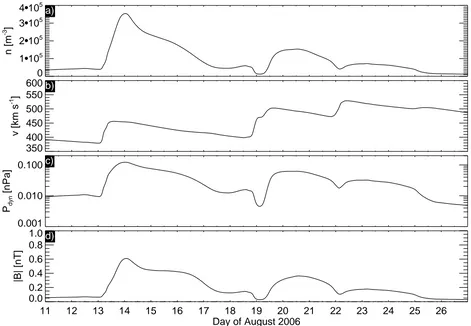
257
is significantly swept-forward. After 23 August 2006 the plasma sheet and lobe period
258
structure returns to that typically found in the magnetotail [Arridge et al., 2009].
259
There is no upstream solar wind monitor at Saturn and so models and propagations from
260
1 AU are often used to infer upstream solar wind conditions [e.g.Zieger and Hansen, 2008;
261
Hsu et al., 2013;Badman et al., 2015;Baker et al., 2009;Jasinski et al., 2014]. Propagation
262
models, e.g., mSWiM [Zieger and Hansen, 2008], which propagate solar wind conditions
263
measured at 1 AU, cannot be used for this interval since Saturn is far from apparent
opposition during this period. In this work we use the ENLIL model, which is a time
265
dependent 3D MHD heliospheric model [Odstrcil et al., 2004] operated at the Community
266
Coordinated Modeling center at NASA Goddard Space Flight Center. This is the only
267
heliospheric model that simulates solar wind conditions beyond 5 AU. ENLIL simulates
268
supersonic, low β plasmas, and must have inner coronal boundary conditions provided
269
by either the Wang-Sheeley-Arge (WSA) [Arge and Pizzo, 2000] (inner boundary located
270
at 21.5 solar radii) or MHD-Around-a-Sphere (MAS) [Riley et al., 2001] (inner boundary
271
located at 30 solar radii) models. The outer boundary can be chosen to extend up to 10
272
AU as appropriate for simulations for Saturn.
273
ENLIL was run using Carrington Rotation 2046 as appropriate for this interval. Figure
274
3 shows the global heliosphere simulation during this period. In Figure 3 we can see
275
density scaled with r2, where r is heliocentric distance, from the heliosphere model. This
276
shows a sequence of compression regions passing over Saturn. In Figure 4 we show a time
277
series of solar wind conditions extracted at Saturn. We can compare the times of high solar
278
wind density shown in Figure 3 with what we see in Figure 4, namely solar wind density,
279
speed, dynamic pressure, and total magnetic field strength in Radial Tangential Normal
280
(RTN) coordinates. These show that this event is included in a solar event compression
281
period. Jian et al. [2011] presented comparisons between ENLIL and Ulysses data at 5
282
AU and showed that the ENLIL predictions for the arrival of solar wind structures had
283
an error of approximately two days. Even if this error is doubled to four days at 10 AU,
284
Saturn is still immersed in a compression region during this event.
285
We also studied Cassini remote sensing data to check if there were increases in activity
286
of Saturn Kilometric Radiation (SKR) emissions and auroras that could support the
simulation results, which suggest that Saturn is immersed in a solar wind compression
288
region [Desch and Rucker, 1983; Kurth et al., 2005; Badman et al., 2008a; Clarke et al.,
289
2009; Kurth et al., 2013]. It has to be considered, anyway, that Stallard et al. [2012]
290
showed a delay of ≃8 h between the arrival of a solar wind compression and brightening
291
of the aurora. In figure 5 we show two auroral images taken by the UVIS instrument on
292
Cassini. The data are projected onto a latitude and local time grid at 1000 km altitude:
293
the figure shows the total FUV intensity, which is predominantly H and H2 emissions.
294
Unfortunately, since Cassini is far from the planet and close to the equatorial plane, the
295
view of the polar region is only partial and at low spatial resolution. Figure 5a shows a
296
bright aurora, seen on the dawnside from 0030 to 0700 local time (with no viewing beyond
297
0700) of the northern hemisphere. The aurora reaches 30 kR between 0100 and 0700 local
298
time from 12◦ to about 16◦ colatitude. Figure 5b shows a more extended aurora: we have
299
two areas, one from midnight to 0600 local time, from about 4◦ to about 20◦, with a
300
brightness between 10 and 30 kR and a second area from 1500 to 1900 local time, from 8◦
301
to about 14◦, with a brightness that reaches ≃ 7 kR. Clarke et al. [2009] reports similar
302
brightness for aurora during disturbed conditions. Since Cassini is far away from Saturn,
303
orbiting in the equatorial plane, the auroral emissions observed by UVIS are subject to
304
significant limb-brightening, whereby the emissions are viewed through a long column of
305
atmosphere near the poles, compared to lower latitudes. This was corrected using the
306
sine of the emission angle, but since each UVIS pixel covers a large area on the planet,
307
the images could still be partially affected by the limb-brightening, which, however, does
308
not affect the extension of the aurora, or the presence of aurora itself. These auroral
309
emissions, the fact that the aurora is extending poleward and is brighter on the dawn
side, suggest that there are some tail dynamics influencing the auroral region and which
311
has been shown to be a consequence of the passage of solar wind compression regions
312
[Stallard et al., 2008; Cowley et al., 2005].
313
Figure 6 shows electric field spectrogram, up to 2 MHz, from RPWS. In this time range
314
the emissions above 3 kHz are Saturn Kilometric Radiation (SKR) and extend until 0600
315
UT on 22 August with low frequency extensions [Jackman et al., 2009]. After this time,
316
narrowband periodic emissions are observed near 5 kHz that are probably generated closer
317
to the planet, hence not likely to be associated with plasma detected near the spacecraft.
318
Narrow band emissions are also observed around 2 kHz, notably at 1530 on 21 August
319
and at 1430 on 23 August, possibly associated with electron plasma oscillations. These
320
can be used to infer the electron density from the frequency which suggests a density of
321
0.05 cm−3, compatible with the CAPS/ELS electron moments. The spectrum below 1.5
322
kHz is noisy, mostly probably given by interference from the spacecraft reaction wheels.
323
However, below about 50 Hz, there are quite visible features (middle of 20 August and
324
just after 06:00 on 21 August) not generated by spacecraft interference. An examination
325
of the corresponding magnetic spectrogram (not shown) shows that these features do not
326
have a magnetic component.
327
More diffuse broadband emissions below 10 Hz might be associated with ionospheric
328
outflow and are seen to correlate with the observation of cold plasma in the tail lobes as
329
identified in figure 2. These emissions may be whistler mode emissions as detected in the
330
magnetotail of Uranus [Kurth et al., 1989]. However, the corresponding magnetic field
331
spectrogram (not shown) does not show a magnetic component to this diffuse broadband
332
emission, suggesting an electrostatic mode.
The SKR observations in Figure 6 show evidence of a brightening in SKR near 1800
334
UT on 20 August as noted by Jackman et al. [2015] and which may be associated with
335
the dipolarization event at 1610 UT reported in that study. SKR emissions are active
336
throughout the rest of the 20 August and 21 August, appearing to switch off early on 22
337
August, clearly showing evidence of magnetospheric dynamics during this period [Desch,
338
1982;Kurth et al., 2005;Badman et al., 2008b;Jackman et al., 2009]. The SKR main
spec-339
trum, which typically ranges between 100-400 kHz, is generated by the cyclotron maser
340
instability. This is in contrast to the lower frequency narrowband emissions mentioned in
341
the previous paragraph which are likely caused by a different mechanism altogether.
342
4. Data analysis
Turning our attention to the specific time interval that we focus on in this case study.
343
Figure 7 is a zoom in of the case study interval, from 1200 to 2400 UT on 21 August,
344
from Figure 2, and shows the characteristics of this event from different instruments on
345
Cassini.
346
Looking at the electron distributions first (Figure 7a) we see that at 1330 on the 21st
347
August (when the spacecraft moves completely into the northern lobe) the population
348
below around 5 eV are trapped spacecraft photoelectrons and the upper edge of this
349
distribution shows that the spacecraft potential is around 5 V. Typically the potential
350
in the lobes is 30-50 V and so this is consistent with the presence of dense plasma in
351
the lobes. From 1330 UT the ambient electron energy drops from 102 eV to a few eV
352
and this ambient population is sometimes hard to distinguish from the trapped spacecraft
353
photoelectron distribution, especially towards the end of the interval. Further evidence of
354
the unique nature of this event is revealed by the low energy of these electrons since in the
quiet tail lobes,Arridge et al.[2009], finds an electron temperature of≃100 eV. Moreover,
356
Figure 8, where we compare two electron spectra, one from this event and one from the
357
magnetosheath, shows how colder the electron population for this event is compared to
358
another region of the magnetosphere.
359
Figure 7b show the ion populations with≃ 3 keV/q ions in the plasma sheet and lower
360
energies in the lobe. The measured ion fluxes are larger than in the plasma sheet and are
361
also seen to slowly disperse in energy from ≃ 500 eV/q to ≃ 100 eV/q over a period of
362
around four hours. During the period in the plasma sheet, the field of view of IMS does
363
not cover the ideal corotation direction and so sees only weak fluxes from directions >
364
30◦ from corotation. However, during the period in the lobes, IMS views flows coming
365
from the direction of Saturn. Figure 9 shows measured ion fluxes as a function of the
366
look direction around the spacecraft, in a polar projection, expressed in OAS coordinate.
367
In this coordinates system S is the axis along the Cassini-to-Saturn line,O is defined by
368
S × (Ω × S), where Ω is the planet spin axis, and A completes the right-hand system.
369
We can represent a point around the spacecraft with two angles relative to the S axis: θ
370
(range from 0◦ to 180◦) is the latitude angle, so it is the polar angle away from Saturn,
371
and ϕ (range from 0◦ to 360◦) is the azimuth around S axis, referenced to 0◦ in the O
372
direction. Specifically in figure 9, θ = 90◦ is represented by the inner circle and θ = 180◦
373
is the outer circle. Hence, these plots show the presence of a cold ion population with a
374
width of ≈40◦ flowing tailward.
375
The ion composition during this interval is also unusual and was determined by a fit
376
of CAPS/IMS time-of-flight data to a forward model [e.g. Thomsen et al., 2010]. In
377
the plasma sheet between 1200 and 1320, where Cassini crosses the plasma sheet twice,
passing from the north lobe to the south lobe, and coming back to the north lobe again,
379
H+ counts are≃104 and (m/q = 2)≃103, and the ratio of water group ions to hydrogen,
380
[W+]/[H+], and m/q=2 to hydrogen, [m/q=2]/[H+], are 1.79 ± 1.58 % and 2.45 ± 0.15
381
% respectively. Hence the plasma sheet appears to be devoid of water group ions. After
382
1320, once the spacecraft is in the north lobe, H+counts are≃105, one order of magnitude
383
larger than the counts of when the spacecraft was crossing the plasma sheet andm/q = 2
384
counts are five times larger. During this time period, the ratio between water group ions
385
and hydrogen [W+]/[H+] is zero within error and [m/q=2]/[H+] = 2.23 ± 0.04 %. From
386
2130 to 2400, the spacecraft returns to the plasma sheet, H+ counts are ≃104, one order
387
of magnitude lower than in the lobes and m/q = 2 counts diminish to 102. During this
388
time period the ratio between water group ions and hydrogen [W+]/[H+] is again zero
389
within error and [m/q=2]/[H+] = 3.22 ± 0.29 %.
390
We checked previous and following spacecraft orbits at the same latitude and the same
391
local time. For the previous orbit (28th July 2006), the lobes are empty of ions and
392
when the spacecraft crosses the plasma sheet twice between 0400 and 1200, [W+]/[H+]≃
393
30.02± 15.11 % and [m/q=2]/[H+] = 24.79±0.26 %. On the following orbit (13th-14th
394
September 2006) the spacecraft seems located always in the lobes, which are mostly empty
395
of ions. Therefore, we consider this an atypical time interval.
396
Looking at MIMI/CHEMS data in Figure 7c and 7d, we find that between 1400 and
397
2030, the lobes are populated by hot H+ with foreground. Hot O+ions start to appear at
398
around 18:45 and they seem slightly dispersed in energy. Higher intensities are observed
399
between 100 and 300 keV, while INCA sees O+ even for larger than 500 keV (see next
paragraph). The pitch angle distribution for this population is generally between 30 and
401
90 degrees, implying an outward flow.
402
Throughout this interval the MIMI/INCA camera is in ion mode and so provides
ad-403
ditional information on the energetic ions. When the spacecraft is in the lobes, we find
404
no O+ during most of the interval. Figure 10 shows O+ distributions observed by INCA
405
from 18:45 to 19:28 and from 20:29 to 21:02.
406
By looking at the INCA look direction and the pitch angle coverage in the columns
407
corresponding to these intervals, we know that, during this time, the spacecraft orientation
408
is steady. Afterwards, we see energy peaks periodically between 18:55 and 19:01, 19:15 and
409
19:28, 19:42 and 19:55 and 20:08 and 20:22, associated with a first order anisotropy, when
410
the spacecraft starts rolling: an entire rotation is enclosed by approximately four white
411
squares corresponding to the period in the intensity peaks [e.g. Kane et al., 2008]. The
412
pitch angle distribution is peaked between 0◦ and 90◦ indicating ions flowing downtail,
413
with scattering accounting for the intensities that appear between 90◦ and 120◦. The
414
highest flux is detected for energies between 89 keV to 589 keV and a very low flux
415
for lower energies, until 20:35, when the O+ covers energies from 46 and 589 keV. The
416
gyroradius for 89 keV to 589 keV ions is ≃ 0.6 to 1.5 RS, hence we interpret the ions
417
before 20:35 as a remote detection of the plasma sheet whilst the spacecraft is the lobes.
418
After this point the spacecraft approaches the plasma sheet (around 20:55) and we see
419
O+ of all energies in the detector; the flow has a broader pitch angle distribution, that is
420
more focused between 0◦and 120◦ with increasing energy. Observing what happens to the
421
magnetic field at the same time, we notice that the magnetic field has lowered, showing
422
a step of about 0.5 nT before 2000 in Br and Btot trend, then a bigger drop in the field
of more than 1 nT. Finally, at 2122 UT, the flux seems to be isotropic and the magnetic
424
field reaches low field strengths, indicating the plasma sheet encounter.
425
INCA observations of H+ are contaminated with O+ due to an instrumental effect but
426
are consistent with isotropic H+ in the lobes and an increasing flux of H+ in the plasma
427
sheet towards the end of the interval.
428
The magnetic field is swept-forward during this all interval, namely Br and Bϕ
compo-429
nents of the field maintain the same sign for more than 8 hours. With a single spacecraft it
430
is difficult to separate spatial and temporal effects and it is possible that this swept-forward
431
field configuration was a characteristic of this local time in Saturn’s magnetosphere. Many
432
of Cassini’s orbits have nearly identical coverage in local-time and latitude so, to check
433
if the field is typically swept-forward at this radial distance and local time, we examined
434
the sweep-back angle during the orbits of Cassini before (28th July 2006) and after (13th
435
and 14th September 2006) the orbit during this case study. The spiral angle of the field
436
indicated that, although the field was generally almost meridional (not swept-forward
437
or swept-back) during these orbits, only this orbit had the swept-forward configuration
438
indicating an unusual configuration.
439
Jackman and Arridge [2011] studied the magnetic field strength in the lobes and
es-440
tablished the average field strength at various radial distances fitting this to a power-law
441
function of radial distance,rin units of RS, such thatBlobe(nT) = (251±22)r−1.2±0.03. At
442
36 RS this expression predicts a field strength of 3.4 ±0.3 nT which is 2 nT smaller than
443
observed, indicating either a highly compressed magnetosphere or where the magnetotail
444
was loaded with open magnetic flux, or both.
5. Interpretation and discussion
In interpreting these observations we have considered several possibilities for the
pres-446
ence of cold ion beams at large distances in Saturn’s magnetotail. Magnetic reconnection
447
would result in rapid ion flows in the range 144-1240 km/s (≃ 10 keV) [Hill et al., 2008;
448
Jackman et al., 2014] and energised electrons in the beam with planetward and tailward
449
ion flows depending on location relative to the X-line. In this case no such energised
450
electrons are observed, the observed ion energies are small, and no large Bθ deflections
451
are observed.
452
In the Saturn system cold plasma usually originates from ionization in the inner
mag-453
netosphere. These cold plasma observations could potentially be the result of rapid cold
454
plasma transport from the inner magnetosphere. In this case, however, we would detect
455
water group ions from the moons and we would expect the ions to be centrifugally
con-456
fined. Furthermore, in our observations we find (W⊥/B≃ 2 eV/nT) and conservation of
457
the first adiabatic invariant implies that we should find a similar ratio close to the source
458
of this ion population. According to Arridge et al. [2011, and references therein], who
459
synthesised the results of many studies, we see that at distance of 5 RS, 8.7 RS and 20 RS
460
we would find respectively a W⊥/B≃ 0.005, W⊥/B≃ 0.3 and W⊥/B≃ 9 eV/nT. Hence,
461
we do not find a ratio ≃ 2 close to the planet. Furthermore, the composition is quite
462
different to what is usually seen in the inner and middle magnetosphere. It is also difficult
463
to envisage a physical mechanism for removing ions from the inner magnetosphere to the
464
tail in the form of a narrow directional ion population.
465
Finally, an alternative interpretation is that we detect Saturn’s plasma mantle: ions
466
that have entered the dayside magnetosphere via dayside reconnection and have mirrored
and flowed out tailward into the magnetotail. We would expect a solar wind plasma
468
composition of [m/q=2]/[H+], namely ≃ 4% which is similar to 2.23 ± 0.04 % from
469
time-of-flight fits. We would also expect the particles to conserve the first adiabatic
470
invariant between the magnetotail and the cusp. From Jasinski et al. [2014] the electron
471
temperature in the cusp is≃40 eV in a field strength of 8 nT, thus W⊥/B≃5 eV/nT, and
472
so we would expect electron energies in the magnetotail to be 25 eV, much higher than
473
observed. At Earth, the electrons in the mantle have same energy as the electrons in the
474
magnetosheath [Formisano, 1980] and we would expect the same to happen at Saturn.
475
Figure 8 shows that the electron population for this event is significantly colder than the
476
electron population in Saturn magnetosheath.
477
Furthermore, we can also examine the convection timescale for newly opened flux tubes
478
compared with the speed of the ions. Assuming a flux tube moves tailward at 40 km/s
479
(≃10% of the solar wind speed) it would take 16.7 hours to traverse the 40 RS from the
480
dayside to the magnetotail. H+ with 1 keV energy would have covered a distance of 436
481
RS in the same time, and the 50 eV H+a distance of about 100 RS. This suggests that by
482
the time the flux tube travels from dayside to the spacecraft position, it would be already
483
emptied of ions. If we considered the rotation time instead (about 5 hours) we would find
484
that 1 keV and 50 eV H+ would travel respectively to distances of 131 R
S and 29 RS.
485
This leads us to not consider valid a mantle provenance for the plasma in our event.
486
5.1. Ionospheric outflow
For ionospheric outflow we would expect cold electrons and ions flowing tailward from
487
Saturn into the magnetotail via the magnetotail lobes, as observed with CAPS/IMS and
488
CAPS/ELS. We would expect the ion composition to be consistent with Saturn’s
sphere, i.e., H+, H+2 and H+3. In the CAPS data, the ions are dominated by H+ with a
490
smaller contribution from a species with m/q=2 which cannot be separated into H+2 and
491
He++. Unfortunately, H+
3 has a time-of-flight in CAPS/IMS which lies near an
instru-492
mental artifact and therefore cannot be extracted at this time. Hence, we interpret this
493
event as ionospheric outflow via a polar wind.
494
It is not possible to determine the connectivity of field lines (open or closed) during
495
the period of ionosopheric outflow. This is a period of intense magnetospheric activity
496
and we think that precipitating electrons producing auroral emissions could happen
si-497
multaneously on the same field line as ionospheric outflow, but still in an upward current
498
region. Hence, the auroral emission and source for ionospheric outflow could be collocated
499
in the same region of the ionosphere. Bunce et al.[2008], used Cassini and Hubble Space
500
Telescope data to show that the Southern auroral oval is located at the boundary between
501
open and closed field lines. However, Jinks et al. [2014], using Cassini data, found that
502
the poleward edge of the upward current region is displaced equatorward from the polar
503
cap boundary in both the northern and southern hemispheres. Thus, the closed field line
504
region can be present also beyond the upward current region poleward boundary. This
505
could imply that the spacecraft was located on closed field lines.
506
Whilst in CAPS/IMS we see cold dispersed ions, we argue that the ions detected in
507
MIMI/INCA and MIMI/CHEMS from 18:45 belong to the plasma sheet: these ions are
508
flowing downtail at speeds ≃1000 km/s. The fact that the plasma sheet is emptied from
509
W+ in the range of CAPS/IMS might suggests that the plasma sheet has been emptied
510
through a reconnection. In this scenario, whilst in the lobes CAPS/IMS detects ions
511
flowing downtail coming from the ionosphere, MIMI/INCA is remotely sensing ions flowing
downtail accelerated by reconnection. Hence, we think that reconnection is happening at
513
the boundary between the lobe and the plasma sheet beneath the spacecraft, while the
514
spacecraft is on open field lines (see Figure 11).
515
According to magnetospheric magnetic field models [Khurana et al., 2006;Bunce et al.,
516
2003], this region of the magnetosphere is only slightly swept-forward, but the
sweep-517
forward increases during periods of increased solar wind dynamic pressure. Since these
518
models only include azimuthal fields due to magnetopause currents, this then shows that
519
the swept-forward configuration is due to magnetopause currents. The reason why we do
520
not see a strongly swept forward configuration in the previous and following orbits, at
521
about same latitude and same local time, is due to the CIR that is passing the planet
522
during this specific time period.
523
Glocer et al.[2007] coupled a polar wind outflow model with an MHD model of Saturn’s
524
magnetosphere to estimate the number flux of ions outflowing from Saturn’s ionosphere
525
in a steady state. They found value between 7.3 × 10⁶ and 1.7 × 108 cm−2s−1. To
com-526
pare our observations with the Glocer et al. [2007] simulations we estimated the number
527
flux, nv, where n is the number density and v is the speed of ions in the tail, and used
528
conservation of magnetic flux to scale these to their values closer to Saturn.
529
The generally low numbers of counts during this event make the ion moment calculations
530
challenging, so we assumed the ion number density was equal to the electron number
531
density. The ion speeds were estimated by fitting the ion spectra with Gaussian plus a
532
background. Fits were filtered using theχ2 for each fit and a manual inspection of the fit.
533
The fits were performed on the IMS anodes where peak fluxes were observed. The peak
534
energy from this fit was taken as the ion bulk flow energy (actually an upper limit since
this assumes the ions are completely cold). The ion speed was found to be ≃400 km s−1
536
at about 1340, with the speed slowly diminishing to get to ≃ 200 km s−1 at about 1700
537
UT.
538
Figure 12 shows the number density, speed, and calculated tail number flux, ntvt. We
539
assumed 10% uncertainty on the electron densities [Arridge et al., 2009]; the speed
uncer-540
tainties were obtained by propagating the uncertainties in the peak energies found from
541
our non-linear fits. The number flux uncertainties were calculated by propagating the
542
uncertainties onnt and vt.
543
Glocer et al. [2007] presented number fluxes at an altitude of 10000 km. To map our
544
observed number fluxes to this altitude, we assume that the number of outflowing ions
545
are conserved in a flux tube from the ionosphere to the tail, and so useBtAt=BiAi, and
546
therefore scale the tail number flux to get the ionospheric number flux bynivi =ntvtBi/Bt.
547
The ionospheric field strength was calculated from a dipole at an altitude of 10000 km at
548
an auroral colatitude of 12◦. Using the observed tail field strength shown in Figure 12d
549
we then calculate the ionospheric number fluxes as shown in Figure 12e. We obtained
550
ionospheric number fluxes between (2.95±0.43)×109 and (1.43±0.21)×1010 cm−2s−1.
551
These estimates are one order of magnitude larger than the value obtained byGlocer et al.
552
[2007].
553
One possible interpretation for this discrepancy is due to the fact that the model was
554
run for a steady atmosphere and steady magnetosphere, hence classical polar wind as
555
defined in Schunk et al. [2007]. We argued that this event occurred during a CIR
(co-556
rotating interaction regions) compression and with substantial magnetospheric activity,
557
which produced enhanced outflows, namely generalised polar wind, as defined in Schunk
et al. [2007]. Moreover, due to low counts it is very difficult to evaluate the velocities
559
with fits that also consider the temperatures. From a preliminary estimate, we think that
560
the speed we calculated overestimate the velocities of a factor of about two. This would
561
affect the number flux of a factor of two, which is a minor contamination for our estimate.
562
In addition, O’Donoghue et al. [2015, and references therein] find a neutral temperature
563
not higher than 650 K, which from Glocer et al. [2007] should lead us to higher values of
564
number flux.
565
We calculated the total particle source rate using the polar cap area range extracted
566
byGlocer et al. [2007], obtaining an estimate between 8.6 ×1028 and 6.3×1029 s−1, that
567
leads to a mass source between 1.4 ×10² and 1.1 ×10³ kg/s, if there were no loss in the
568
tail.
569
By contrast, using the mean position of the northern and southern aurora (respectively
570
15.1±1.0◦ and 15.9±1.9◦, Carbary [2012]) we can recalculate the area of the polar cap
571
and we obtain instead a rate of 49.1 ±9.8×1027 and 23.7 ±4.7×1028 s−1, and a mass
572
source between 82.0±16.5 and 395.6±79.2 kg/s.
573
If we considered instead, more realistically, an active area covering the region of
auro-574
ral emission (northern and southern extending respectively between 13.4◦ and 16.8◦ and
575
between 12.9◦ and 18.9◦, average values taken from Carbary [2012]), we would obtain
576
a source rate between 29.7 ±8.1×1027 and 14.3 ±3.8×1028 s−1 (mass source between
577
49.7±13.4 and 239.8±64.8 kg/s).
578
Specifically for our event, we can see, from UVIS data, the active area from auroral
579
emissions in the hours prior the event: it extends from 5◦ and 12◦, from 0000 to 1900
580
LT, with a data gap from 0600 to 1430 LT. If we considered an outflow only from the
brightest area (we then consider the area of the ring which includes the brightest area
582
from dawn to dusk, divided by two to consider the area with no auroral emission and the
583
data gap) with an estimated error of 2.5◦ (half of the projected polar grid resolution), we
584
would obtain 6.1 ±2.9×1027 and 2.9 ±1.4×1028 s−1 for a total mass source between of
585
10±4 and 49±23 kg/s.
586
Evaluating the fact that the whole auroral oval is not completely active in our event
587
and the active area has a different brightness, so possibly the outflow is not coming out
588
uniformly, a useful quantity to be defined is the rate and the mass source per hour of local
589
time, spanning 5◦ in latitude (in our event mainly from 5◦ and 10◦): 3.2±1.9×1026 and
590
1.5 ±0.9×1027 s−1 per hour of local time, hence between 0.5±0.3 and 3±1.5 kg/s per
591
hour of local time.
592
The mass source estimates for different active areas are here calculated only for the
593
northern cap, the northern auroral and the aurora in the north pole we remote sense with
594
Cassini/UVIS. Moreover, the source rates calculated are upper limits of the ionospheric
595
mass contribution to the magnetosphere: we do not have any estimate at the moment on
596
how much of this mass stays indeed in the magnetosphere.
597
The ion dispersion can be generated by three different processes, two of them consisting
598
in a temporal variation and one of them in a spatial variation. The first temporal effect
599
is due to the fact that the energies of the particles emitted from the same area in the
600
ionosphere, have a Maxwellian distribution. Consequently, there is a velocity filter effect
601
whereby faster ions reach the spacecraft before slower moving ions, producing a continuous
602
velocity dispersion in the data. The second temporal scenario can be caused by a time
603
variability of the source. Therefore the spacecraft, in this case, would be detecting ions
originated from the same source, but a source that was in an exited state at the beginning
605
of the time interval, and then relaxed afterwards, emitting lower energy ions towards the
606
end of the interval. Lastly, the spatial scenario could be caused by the fact that the
607
spacecraft moves across different field lines which have their feet in different latitudes
608
in the ionosphere. At the beginning of the interval, the spacecraft would have been
609
located on a field line connected to an intensely exited region of the ionosphere, and
610
then the spacecraft moved onto field lines connected to a calmer region of the ionosphere.
611
Unfortunately, from the data is not possible to distinguish among these three different
612
scenarios. A combination of two or all of these processes may be involved in producing
613
the observed ion energy dispersion.
614
We know the presence of an electron dispersion in the data, maybe produced by the
615
same process that caused the ion dispersion.
616
If we interpret the ion dispersion as a velocity filter effect, whereby faster ions reach
617
the spacecraft before slower moving ions from a spatially-restricted source, then we can
618
obtain the distance to that source from a time-of-flight expression t = t0 +d/v, where
619
t is the time of observation, t0 is the time at which all the ions left the source, v is the
620
speed of an ion observed at time t, and d is the distance to the source. We used the
621
velocities and times from Figure 12, calculated the inverse velocity, and then fitted a
622
straight line to t as a function of 1/v to obtain the intercept (t0) and the gradient (d).
623
Thereforedis an estimate of the field-aligned distance that the ions travelled and the time
624
at which they left their source t0. The ion counts were not considered to be sufficiently
625
far above background to perform this analysis using energy-time spectra and, hence, we
626
have performed the moment analysis as an alternative. The distance was found to be
69 ± 3 RS. Considering that our speeds are possibly over-estimated by a factor of ≃ 2. 628
we then obtain a distance of 34± 1 RS. This is consistent with the length of a field line
629
from Cassini to Saturn’s ionosphere calculated by tracing field lines in a magnetospheric
630
field model Khurana et al. [2006], thus strengthening the interpretation of this event as
631
ionospheric outflow.
632
6. Conclusions
We presented a case study of an event from Saturn’s magnetotail from 21 August (day
633
of year 233) 2006. The event is enclosed in a time period when the magnetosphere was
634
compressed by a region of high solar wind dynamic pressure, as identified from a global
635
heliosphere simulation (ENLIL) and auroral and SKR intensifications. Cold ions and
636
electrons are detected in the lobes and the cold plasma ion composition does not show
637
evidence for W+ ions, neither when the spacecraft is located in the plasma sheet or when
638
Cassini is in the lobes.
639
After considering different interpretations, we conclude that this event is an example
640
of ionospheric outflow in Saturn’s magnetotail. This is the first time that a low-energy
641
ionospheric outflow event has been detected at planets other than Earth, helping
un-642
derstand how ionospheric outflow contributes to the magnetosphere. We estimate an
643
ionospheric escape number flux (at an altitude of 10000 km) between (2.95±0.43)×109
644
and (1.43±0.21)×1010 cm−2s−1 one or two orders of magnitude larger than the estimate
645
obtained byGlocer et al.[2007], which represents a mass source between 1.4 ×10² and 1.1
646
×103 kg/s. Furthermore, we estimated the mass source provided by the ionosphere, for
647
different configurations of the active region at the northern pole. Considering the most
648
source between 49.7±13.4 and 239.8±64.8 kg/s, comparable with what was found for
650
Enceladus (60-100 kg/s [Fleshman et al., 2013]). Specifically for the auroral morphology
651
found during this event, we obtained a mass source between of 10±4 and 49±23 kg/s.
652
However, we do not have any current estimate on how much of the mass provided by the
653
ionosphere, stays indeed in the magnetosphere and how much instead gets lost downtail.
654
As such, our estimates are an upper limit to the magnetospheric mass source.
655
Future work will include a survey to search for evidence of other ionospheric outflow
656
events at Saturn; besides modelling ionospheric outflow from Saturn’s ionosphere with a
657
dynamic magnetosphere and atmosphere is needed to understand the relationship between
658
reconnection or magnetosphere-ionosphere coupling and the outflow from the atmosphere.
659
Moreover, other interesting steps could involve an estimate how much of the mass flowing
660
in the tail from the ionosphere remains in the magnetosphere and how much is lost
down-661
tail. A search for evidence of low energy H+3 in the magnetosphere will also provide further
662
evidence for ionospheric outflow. Cassini proximal orbits during its Grand Finale at the
663
end of mission will provide complementary measurements to place better constraints on
664
the ionosphere as a mass source at Saturn. These studies will also provide a valuable
665
context before Juno’s arrival at Jupiter.
666
Acknowledgments. MF was supported in this work by Il Circolo, the European Space
667
Agency, the Royal Astronomical Society, Agenzia Spaziale Italiana, and the Science and
668
Technology Facilities Council. MF completed this work whilst a visiting student at
Lan-669
caster University and would like to thank the Department of Physics, staff and students,
670
for their kindness and support. MF would like to thank Rob Wilson, K.C. Hansen, Tamas
671
Gombosi, Elias Roussos, Doug Hamilton, Frank Crary, Krishan Khurana, Norbert Krupp