warwick.ac.uk/lib-publications
Original citation:
Filippou, Ilias, Gozluklu, Arie Eskenazi and Taylor, Mark P. (2018) Global political risk and currency momentum. Journal of Financial and Quantitative Analysis.
Permanent WRAP URL:
http://wrap.warwick.ac.uk/96779
Copyright and reuse:
The Warwick Research Archive Portal (WRAP) makes this work by researchers of the University of Warwick available open access under the following conditions. Copyright © and all moral rights to the version of the paper presented here belong to the individual author(s) and/or other copyright owners. To the extent reasonable and practicable the material made available in WRAP has been checked for eligibility before being made available.
Copies of full items can be used for personal research or study, educational, or not-for profit purposes without prior permission or charge. Provided that the authors, title and full bibliographic details are credited, a hyperlink and/or URL is given for the original metadata page and the content is not changed in any way.
Publisher’s statement:
This article has been accepted for publication in a revised form
https://www.cambridge.org/core/journals/journal-of-financial-and-quantitative-analysis A note on versions:
The version presented here may differ from the published version or, version of record, if you wish to cite this item you are advised to consult the publisher’s version. Please see the ‘permanent WRAP URL’ above for details on accessing the published version and note that access may require a subscription
Political Risk and Currency Momentum
∗
Ilias Filippou Arie E. Gozluklu Mark P. Taylor
This version: December 19, 2017
∗Acknowledgments: Filippou, Ilias.Filippou@wbs.ac.uk, Warwick Business School, The University of
Political Risk and Currency Momentum
Abstract
Using a measure of political risk, relative to the U.S., that captures unexpected political conditions, we show that political risk is priced in the cross section of currency momentum and contains information beyond other risk factors. Our results are robust after controlling for transaction costs, reversals and alternative limits to arbitrage. The global political envi-ronment affects the profitability of the momentum strategy in the foreign exchange market; investors following such strategies are compensated for the exposure to the global political risk of those currencies they hold, i.e., the past winners, and exploit the lower returns of
loser portfolios. The risk compensation is mainly justified by the different exposures of for-eign currencies in the momentum portfolio, to the U.S. political shocks, which is the main component of the global political risk.
Keywords: Currency Momentum, FX Risk Premium, Limits to Arbitrage, Political Risk.
1.
Introduction
In this paper we report research on the role of political risk in the foreign exchange (FX)
market and in particular on the issue of how political shocks influence currency investment
strategies and affect their profitability. The FX market is a global decentralized market for
the trading of currencies against one another and it is by far the largest financial market in
the world in terms of both geographical dispersion and daily turnover, which is in excess of $5
trillion.1 Nevertheless, despite its size and global importance, the FX market is perhaps one
of the least well understood financial markets. For example, while there is some evidence
that standard macroeconomic variables may influence the long-run behavior of real and
nominal exchange rates, the shorter term disconnect between fundamentals and exchange
rate movements is well documented (see, e.g.,Taylor,1995). Similarly, significant departures
from the simple (i.e. risk-neutral) efficient markets hypothesis for FX, according to which
uncovered interest parity (UIP) should hold and the forward rate should be an optimal
predictor of the future spot exchange rate, are also well documented (see, e.g.,Hodrick,1987;
Froot and Thaler,1990;Taylor,1995;Sarno and Taylor,2002, for surveys of this literature).
Indeed, there is evidence that traders in the FX market have been able to exploit the failure
of UIP to pursue profitable trading strategies based on the carry trade (buying high-interest
rate currencies against low-interest rate currencies), as well as profitable strategies based on
value (selling currencies that appear to be overvalued against currencies that appear to be
undervalued according to some fundamental value measure such as purchasing power parity)
and momentum (buying currencies that have recently been rising in value against currencies
1According to the last Bank for International Settlements’ Triennial Survey, daily turnover in the global
that have recently been falling in value) (see, e.g., Rime and Schrimpf, 2013).
An investor who follows a momentum strategy buys a basket of currencies that
per-formed relatively well in the past (winners) while short-selling currencies with relatively
poor past performance (losers); this naive strategy renders high annualized Sharpe ratios
and is uncorrelated with the payoffs of other strategies, such as value or carry (Burnside,
Eichenbaum, and Rebelo, 2011a; Menkhoff, Sarno, Schmeling, and Schrimpf, 2012b). Its
profitability could partially be explained by transaction costs, limits to arbitrage or
illiq-uidity.2 However, to the best of the present authors’ knowledge there is no successful FX
asset pricing model that explains both the times-series and the cross-sectional dispersion
of currency momentum returns. We attempt to remedy this by investigating how global
political shocks may influence currency momentum strategies since there has been limited
success to explain their profitability and we argue there may be good reason to suspect that
momentum may be influenced by political stability. The absence of a ”tangible”
fundamen-tal anchor (e.g., Stein, 2009; Lou and Polk, 2013) leads to more unstable profitability and
more pronounced vulnerability of momentum strategies to limits to arbitrage. Existing risk
factors that have been able to capture the profitability of other currency strategies have been
shown not to have a first-order effect on currency momentum returns either in times-series
or in cross-sectional dimensions (e.g., Menkhoff et al., 2012b). Conversely, we show that
while political risk has a first-order effect on momentum, it does not have a first-order effect
on other currency strategies such as carry and value, as other risk factors explaining those
strategies are dominant.
To analyze the question as to whether global political risk prices the cross section of
2In particular,Menkhoff et al.(2012b) show that momentum exhibits a significant time-variation that is
currency momentum returns, we develop a novel measure of political risk that captures
differences between the political environment of the U.S. economy and that of the rest of
the world. A striking feature of this measure is its sensitivity to unexpected global political
changes, meaning that it captures political events that are less likely to be predicted, certainly
by a naive investor.3 We thus examine whether global political shocks affect the profitability
of momentum strategies, which helps us understand better the determinants of currency
risk premia. We construct a two-factor asset pricing model that incorporates information
contained in our global political risk measure. More precisely, the first factor is alevel factor
as originally introduced by Lustig, Roussanov, and Verdelhan(2011), which is measured as
the average return across portfolios in each period. This traded factor resembles a strategy
that buys all foreign currencies and sells the U.S. dollar. As such, it is highly correlated
with the first principal component of currency excess return portfolios. The second (slope)
factor is our global political risk measure, designed to capture political risk surprises around
the world; this factor is highly correlated with the second principal component of currency
momentum portfolios. We find that global political risk is priced in the cross section of
currency returns since it is able to explain a significant part of currency excess returns.
Winner portfolios load positively on global political risk innovations while loser portfolios
load negatively. Our main intuition regarding this finding is linked to the fact that investors
require a higher premium for taking on global political risk by holding a portfolio of past
winner currencies. On the other hand, investors accept a lower return from investing inloser
portfolios, i.e. past loser currencies, as they provide insurance against adverse movements
of currency returns in bad states of the world. From the perspective of currency momentum
investors, bad states of the world are characterized either by increases in political risk in the
3A good example is the Brexit referendum outcome on 23rd June 2016 which caught the market
U.S. or decreases in political risk in the foreign country. We mainly focus on momentum
strategies that rebalance portfolios every month and use formation periods of one, three and
six months; the main reason for focusing on these particular strategies is related to their
high profitability (Menkhoff et al., 2012b).4
First, we show that global political risk can explain both time-series and cross-sectional
currency momentum returns even after controlling for other predictors in the literature such
as global FX volatility, FX liquidity, FX correlation and changes in credit default swap (CDS)
spreads. Notably, the predictability mainly comes from loser portfolios along the time-series
dimension, although it captures only a small part of the time-series variability. Next, we
question whether political risk is able to capture the cross-sectional variation of currency
premia that it is related to currency momentum. We find that momentum returns sorted into
portfolios based on exposures to political risk provide an almost monotonic pattern, which
suggests that investors require a higher premium when currency exposure to political risk
increases. In particular, the extreme portfolios render a positive spread that indicates the
pricing ability of global political risk. This spread can be explained by the fact that global
political risk cannot easily be diversified away in a currency momentum strategy because, by
construction, momentum portfolios consist of currency pairs with correlated past returns.
Our asset pricing model exhibits strong cross-sectional performance both in statistical
and in economic terms. In particular, we analyze the results of Fama and MacBeth (1973)
regressions as well as generalized method of moments (GM M) procedures (Hansen, 1982),
and find highly significant risk-factor prices that are related to global political risk. Our
results also demonstrate strong cross-sectional behaviour in terms of goodness of fit.
Specif-ically, we show that we cannot reject the null hypothesis that all of the pricing errors are
jointly equal to zero, as signified in terms of very large p-values of the χ2 test statistic: we
cannot reject the null hypothesis that the HJ distance (Hansen and Jagannathan, 1997) is
equal to zero and the cross-sectional R2 ranges from 66% to 99% for formation periods from
one to six months. The results are similar whether we employ a mimicking portfolio or the
raw measure.
We then examine whether global political risk is priced even after accounting for other
determinants of currency premia. We start with idiosyncratic volatility and skewness so as to
determine whether we can explain different sources of limits to arbitrage. Thus, we
double-sort conditional excess returns into two portfolios based on their idiosyncratic volatility or
idiosyncratic skewness. Then within each portfolio, we sort them according to their exposure
to global political risk. We find that currency excess returns are larger in high political risk
portfolios than in low political risk baskets under low or high idiosyncratic volatility
portfo-lios, implying a statistically significant and positive spread. We perform similar exercises by
replacing idiosyncratic volatility with illiquidity, volatility and a correlation variable (e.g.,
Mueller, Stathopoulos, and Vedolin,2013) and reach the same conclusion. These results
pro-vide further support for the pricing ability of global political risk for currency momentum.
Finally, we perform additional robustness checks. In oder to make our analysis more
realistic, i.e. applied totradable strategies, we apply two filters to the data: (i.) we exclude
currencies of the fixed exchange rate regime, and (ii.) include only those with a high degree of
capital account openness (Chinn and Ito,2006; Della Corte, Sarno, Schmeling, and Wagner,
2013). We find that the results are improved in most cases. In addition, we show that
allowing for the implementation cost of the strategies does not affect the cross-sectional
predictive ability of global political risk. We also ask whether currency reversals could
by using as the conditional variable the previous month’s momentum return. Again, we find
that the results are largely unaffected. Finally, we perform currency-level cross-sectional
regressions for conditional returns and again demonstrate the pricing ability of global political
risk.
Overall, our empirical evidence suggests that global political risk is able to capture most
of the dispersion of currency momentum returns. This finding suggests that political risk
is one of the fundamental determinants of the momentum strategy in the foreign exchange
market. Finally, we show that political risk is present in other currency strategies, such as
carry trades and currency value, but it does not have a first-order effect, as other risk factors
explaining those strategies are dominant.
The remainder of the paper is set out as follows. In section 2 we set out a brief review
of the literature on political risk and currency momentum, while we define and discuss our
global political risk measure in section 3. In section 4 we provide a brief description of
the data as well as the construction of the currency portfolios. Section 5 discusses the
empirical results of the paper. In section 6 we attempt to provide a better understanding
of the underlying determinants of currency premia. Section7offers some robustness checks.
Finally, in section 8, we provide some concluding remarks.
2.
Related Literature
In this section we review related studies on political risk and currency momentum in order
to set the scene for our investigation. We begin by examining some salient studies linking
political risk to the foreign exchange market before turing to the link between to political
risk and currency momentum more specifically. While precise interpretations of political
political risk to “unwanted consequences of political activity” and the second links it to
political events.
Political Risk. There is an established body of literature on the relation between exchange
rates and political risk. In early contributions to this literature, Aliber (1973) and Dooley
and Isard(1980) consider two main channels of risk that could be linked to deviations from
the UIP condition, namely, exchange rate risk and political risk. This separation is further
analyzed by Dooley and Isard (1980), who focus on the role of capital controls and the
political risk premium. In addition, Bailey and Chung (1995) study the role of political
risk and movements in exchange rates in a cross section of stock returns in Mexico, finding
evidence of risk premia that are associated with these risks. Moreover, Blomberg and Hess
(1997) find that an FX forecasting model incorporating political risk variables can beat a
random walk in an out-of-sample forecasting exercise for three currency pairs.
Political Events. Another strand of this literature focuses on political risk premia
asso-ciated with political news. For example,Boutchkova, Doshi, Durnev, and Molchanov(2012)
investigate how stock market volatility broken down by industry is influenced by both local
and global political uncertainty. Pastor and Veronesi (2012) study the influence of
gov-ernment policies on stock prices and show that political risk related to announcements of
policy changes should lead to a drop in equity prices on average, with an analogous increase
in volatility and correlation. In addition, Addoum and Kumar (2013) develop a trading
strategy that exploits changes in political events, such as U.S. presidential elections or the
beginning and end of a presidential term, demonstrating that investors require a premium
under those periods because political uncertainty is higher. Lugovskyy (2012) employs a
there is political regime change risk that varies depending on the government under control.
Kelly, Pastor, and Veronesi (2014) show that political uncertainty is priced in the options
market such that options with maturity around political events appear to be more
expen-sive.5 We deviate somewhat from these studies as we do not focus on specific political events
but, rather, we attempt instead to capture unexpectedchanges in the political environment
that drive currency premia.
Currency Momentum. Recent analyses of currency momentum in the foreign exchange
rate market research literature include Okunev and White (2003), Burnside, Eichenbaum,
and Rebelo (2011a), Menkhoff et al. (2012b) and Asness, Moskowitz, and Pedersen(2013),
each of which focuses on the cross-sectional dimension of the momentum strategy. Most
of the earlier studies focus on time-series momentum, often labeled as a form of “technical
analysis”.6 Our methodology is closely related to that one employed by Menkhoff et al.
(2012b). In regard to the performance of momentum strategies, Cen and Marsh (2013)
show that momentum was more profitable in the interwar period, and provide out-of-sample
evidence of profitability for a period that could be characterized by rare events. Menkhoff
et al. (2012b) also show the disconnection between equity and currency momentum as well
as the low correlations between carry and momentum returns. Bae and Elkamhi (2014) find
that a global eqyuity correlation factor jointly explains carry and momentum portfolios in
the FX market. Our analysis is different as our factor provides a fundamental determinant
of currency momentum. Barroso and Santa-Clara(2013) show that in the equities market an
investor could avoid momentum crashes by hedging against momentum-specific risks rather
5For other measures of uncertainty please seeGao and Qi (2012);Julio and Yook(2012);Baker, Bloom,
and Davis(2012);Belo, Gala, and Li (2013);Cao, Duan, and Uysal(2013).
6Surveys of FX market practitioners by Taylor and Allen (1992) and Cheung and Chinn (2001) show
than market risk. Asness, Moskowitz, and Pedersen (2013) document the prevalence of
value and momentum returns across a range of asset classes (including FX) and the negative
correlation between value and momentum; insofar as political risk may be expected to impact
negatively on expected value, this would suggest that political risk may generate momentum
as investors demand a premium for investing in relatively high political risk currencies.
3.
Relative Political Risk
In this section we discuss the role of global political risk in the foreign exchange market
and attempt to provide a deeper understanding of the channel through which political risk
enters into the currency market and affects investors’ decisions. We also define our measure
of political risk and analyze its dynamics.
Menkhoff et al. (2012b) show that currency momentum is mainly concentrated in
coun-tries that are less developed and exhibit a high risk of employing capital controls that could
inflate the volatility of the exchange rate. On the other hand developed countries exhibit
very low profitability for momentum trading, supporting this finding. Thus, it is apparent
that currency momentum may be subject to limits to arbitrage while its profitability is
heav-ily determined by country-specific characteristics. For example, these authors demonstrate
that momentum exhibits a particular time-variation that stems from country-specific shocks
and will thus be more pronounced in highly idiosyncratic volatility portfolios.
Political risk is one of the main determinants of country-specific shocks. For example,
P´astor and Veronesi (2013) employ a general equilibrium model to show that in economies
with a weak economic profile, political uncertainty requires a risk premium to asset returns
that should increase as the economic conditions deteriorate. Boutchkova et al. (2012) also
are concentrated in periods characterized by a large idiosyncratic volatility. We should
recall that currency momentum is more extreme in periods of high idiosyncratic volatility
(Menkhoff et al., 2012b) which verifies our assumption regarding the role of political risk
in the momentum strategies. Moreover, Lensink, Hermes, and Murinde (2000) show that
political risk is a strong determinant of capital flight.7 Therefore, it is apparent that political
risk could serve as a candidate risk factor for currency momentum, since it is a
forward-looking measure that heavily affects currency premia in comparison to other country-specific
characteristics when country risk is high.
We introduce a novel measure of global political risk that it is defined relative to U.S.
political conditions and is designed to capture differences between the political uncertainty
of the U.S. and the rest of the world.8 It is natural to think of political risk relative to the
U.S. for two reasons. First, we are dealing with U.S. dollar exchange rates against other
currencies and so, although we will for the most part analyze portfolios of currency returns
rather than individual currency returns, we will still need a relative measure to reflect the
bilateral nature of exchange rates. Second, the role of the U.S. dollar as the global reserve
currency, as well as the dominance of the United States in financial markets as well as the
global political economy (e.g. the strong effect of U.S. interest rate movements on emerging
market capital flows and the U.S. military influence on NATO countries), suggests that a
measure of global politcal risk relative to the U.S. is appropriate for analyzing global financial
markets in general and currency markets in particular.
We build our measure of global political risk starting with a measure at the country
level, which we obtain from the International Country Risk Guide (ICRG) published by the
7For further examples seeAlesina and Tabellini(1989).
8Bekaert, Harvey, Lundblad, and Siegel (2014) construct a similar measure to proxy for political risk
PRS Group. The ICRG political risk rating is a long-running dataset, produced monthly
for the last three decades and covering over 140 countries, and is widely used in the finance
industry as a means of assessing the political stability of countries on a comparable basis.
Each month, ICRG country experts assign risk points to a preset group of 12 factors, termed
political risk components, by collecting information on each component and converting these
into risk points on the basis of a consistent pattern of evaluation.9 Specifically, our proxy
for global political conditions is measured by:10
PRt≡
1
nt nt X
i=1
PRi,t
z }| {
pri,t−prU S,t
σPR
i,t
, (1)
where nt is the total number of available currencies at time t and pri,t represents our
for-eign (country i) measure of political risk and prU S,t the US measure, each at time t. The
ICRG political risk measure is constructed such that an increase in the measure denotes a
reduction in political risk; thus, we use the log reciprocal of the ICRG measure for country
j, pr(ICRG)j,t, say, in order to have a measure that increases with political risk, i.e. prjt ≡
ln (1/pr(ICRG)j,t). The denominator in (1), σPRi,t , is the cross-sectional average of the time
tabsolute deviation of the foreign (i-th country) measure of political risk from the U.S.
mea-sure.11 We normalise the numerator in (1) with the cross-sectional absolute average political
risk on a month-to-month basis so as to highlight country risk relative to global political
9For further details of the PRS Group, see https://www.prsgroup.com/; for full details of the ICRG
methodology, see http://www.prsgroup.com/wp-content/uploads/2012/11/icrgmethodology.pdf. The 12 weighted variables are: government stability, socioeconomic conditions, investment profile, internal conflict, external conflict, corruption, military in politic, religious tensions, law and order, ethnic tensions, democratic accountability and bureaucracy quality. In turn, each of these is broken down into subcategories.
10We also account for differences inglobalisationacross countries by creating a value-weighted global
polit-ical index, based upon the ICRG risk ratings weighted according to weights determined by the KOF Index of Globalization (http://globalization.kof.ethz.ch/), and we find that the two measures behave similarly. The value weighted index is available upon request.
11i.e. 1 nt
Pnt|pr
conditions; this is useful because it gives us the opportunity to capture the simultaneous
deterioration of political conditions between countries with similar characteristics and vice
versa.12
While (1) gives a measure of global political risk, our focus is on global political risk
innovations (denoted ∆PRt), which we measure as the innovations obtained from a
first-order autoregressive model for PRt.13 Figure 1 graphs ∆PRt over the period January
1985 to January 2014. Note that a positive value of the innovation represents less political
risk associated with the U.S. relative to the rest of the world, and conversely when the
innovations are negative. We have also picked out a number of extreme movements in the
risk innovations, where they are apparently related to well known political events, and these
are labeled in Figure 1.
[Figure 1 about here.]
Figure A1 in the Internet Appendix provides a graphical illustration of our global political
risk innovations along with other risk factors employed in the literature such as global FX
volatility (as in Menkhoff, Sarno, Schmeling, and Schrimpf, 2012a), global FX correlation
(e.g. Mueller, Stathopoulos, and Vedolin, 2013)), global FX liquidity innovations (measured
as global bid-ask spread (similarly to Menkhoff et al., 2012a, section 4) and global CDS
spreads (measured as differences of average CDS spreads across countries, e.g. Della Corte
et al., 2013). We see that our measure does not have a strong business cycle component and
other risk factors in the foreign exchange market are unrelated to our measure, indicating
that we are attempting to capture different dynamics of currency premia.14
12In the robustness section, we explore alternative definitions of global political risk by omitting the
normalisation factor, expanding the set of foreign countries or focusing only on U.S. political risk.
13Alternatively, one could compute ∆PR
t by taking first differences rather than innovations. Our results
remain similar regardless of the method being used and they are available upon request.
Table1reports descriptive statistics of our global political risk innovations as well as other
risk factors in the literature such as innovations to global FX volatility, global FX correlation,
global FX illiquidity and global CDS spreads changes. In accordance with Figure A2, we find
that global political risk is uncorrelated (Corr) with other factors even when we take into
consideration the time-variation in the correlation structure by employing rolling correlations
based on a 60-month rolling window. In particular, M axCorr (M inCorr) represents the
most extreme positive (negative) correlation of global political risk innovations with each of
the other variables. Moreover, our political risk measure demonstrates low persistence
(first-order autocorrelation of 0.09), exhibiting negative skewness and excess kurtosis. Likewise,
all the remaining measures exhibit low persistence as they are measured in a similar way.
[Table 1 about here.]
Figure A3 in the Internet Appendix shows the correlation of country-level political risk
innovations with respect to U.S. innovations over the sample period. We first note that the
correlations are on average low and seldom exceed 25 percent, exceptions being in cases where
countries have significant political ties with the U.S., such as the U.K., Canada, Kuwait,
Saudi Arabia, Egypt and Russia. In order to understand the source of the correlations we also
report in Figure A4 of the Internet Appendix correlations of innovations to each individual
component of political risk index relative to U.S. components of political risk. We see that the
investment profile component which covers aspects related to contract expropriation, profits
repatriation15 or payment delays dominates in terms of significant correlations. Nonetheless
measure is not related with any business cycle variation of any other country in our sample. Particularly, we follow Bauer, Rudebusch, and Wu(2014) and proxy the business cycle variation of the countries in our sample with the leading indicators of OECD (OECD plus six NME). After projecting our global political risk measure on the changes of the OECD leading indicator, we find that there is no contemporaneous or lagged relation between the two measures, indicating the disconnection of our variable with the business cycle.
15For example, firms tend to consider the tax jurisdiction in order to allocate their earning abroad or
correlations remain low across different components.16
4.
Data and Currency Portfolios
In this section, we provide a detailed description of the data used in our research as well as
describe the construction of our momentum strategy portfolios.
Exchange Rate Data. We begin with daily spot and one-month forward exchange rates
against the U.S. dollar spanning the period January 1985 to January 2014. The data are
collected from Barclays and Reuters via Datastream. Transaction costs are taken into
con-sideration through the use of bid, ask and mid quotes. We construct end-of-month series
of daily spot and one-month forward rates as in Burnside, Eichenbaum, Kleshchelski, and
Rebelo (2011). The main advantage of this approach is that the data is not averaged over
each month but represents the rate on the last trading day of each month. The sample
is similar to the one employed by Menkhoff et al. (2012a,b) and comprises 48 countries.17
We apply various filters in the data so as to make the analysis more realistic, focusing on
implementable strategies.18
2012;Bennedsen and Zeume,2015). This practice, in principle, could affect currency flows between countries with different tax environments.
16In Figure A5 of the Internet Appendix, we show the turnover of portfolios sorted based on global political
risk. The majority of the countries appear in extreme portfolios.
17Australia, Austria, Belgium, Brazil, Bulgaria, Canada, Croatia, Cyprus, Czech Republic, Denmark,
Egypt, Euro area, Finland, France, Germany, Greece, Hong Kong, Hungary, India, Indonesia, Ireland, Israel, Italy, Iceland, Japan, Kuwait, Malaysia, Mexico, Netherlands, New Zealand, Norway, Philippines, Poland, Portugal, Russia, Saudi Arabia, Singapore, Slovakia, Slovenia, South Africa, South Korea, Spain, Sweden, Switzerland, Taiwan, Thailand, Ukraine, United Kingdom.
18Those currencies that were partly or completely pegged to the U.S. dollar are not excluded from the
Currency Excess Returns. We denote by St and Ft the level of the time t spot and
forward exchange rates, respectively. Each currency is quoted against the U.S. dollar such
that an appreciation of the U.S. dollar reflects an increase inSt. The realized excess return
(RXt+1) is defined as the payoff of a strategy that buys a foreign currency in the one-month
forward market at timetand then sells it in the spot market at maturity at time t+ 1.19 The
excess return can be computed asRXt+1 ≡ Ft
−St+1
St =
Ft−St
St −
St+1−St
St .Thus, the excess return
can be decomposed into two components; the forward discount and the exchange rate return.
Moreover, the covered interest-rate parity (hereafter CIP) condition implies that the forward
discount is a good proxy for the interest rate differentials, i.e. (Ft−St)/St 'ˆit−it, where
ˆit and it denote the foreign and domestic riskless interest rates, respectively.20 Therefore,
the excess return could also be written as RXt+1 ' (ˆit−it)−(St+1−St)/St. In the latter
expression, the currency excess returns can be approximated by the exchange rate exposure
subtracted from the foreign-domestic risk-free interest rate differential. The implementation
cost of the currency strategy is taken into consideration though the use of bid and ask spreads.
Particularly, buying the foreign currency forward at timetusing the bid price (Ftb) and selling
it at time t+ 1 in the spot market at ask price (Sta) is given by: RXtl+1 = (Ftb −Sta+1)/Stb.
Whereas the corresponding short position in the foreign currency (or short in the dollar)
will render a net excess return of the form: RXs
t+1 =−(Fta−Stb+1)/Sta. We report results
with and without transaction costs because the inclusion of bid and ask quotes inflates the
volatility of the excess returns, giving more weight to less traded and illiquid currencies.21
Malaysia from August 1998 to June 2005 and Indonesia from December 2000 to May 2007.
19The excess return is in fact thetotal return to such a strategy as it involves a zero commitment of funds. 20Taylor (1987, 1989) and more recently Akram, Rime, and Sarno (2008) provide a detailed empirical
examination of the CIP condition and show that it holds at daily and lower frequencies.
21Neely and Weller (2013) argue, based on interviews with traders, that posted bid-ask spreads may
Political Risk Data. Our measure of country-level political risk (i.e. pri,t) is constructed
using data from the International Country Risk Guide (ICRG). As noted earlier in Section
3 where we describe the construction of our political risk measure in detail, we compute
the log inverse of the ICRG measure in order to obtain a measure that increases with with
political risk. We then construct our global political risk measure relative to the U.S., PRt,
as in equation (1) and obtain our global political risk innovations measure, ∆PRt, from the
fitted innovations in anAR(1) model for PRt.
Momentum Portfolios. At the end of each month t, we allocate currencies into six
portfolios on the basis of their past performance obtained at time t-f, where f represents
the formation period and each portfolio is held for a month (h). To this end, the first
Portfolio contains the worst performing currencies (i.e. losers) and the last basket consists
of the winner currencies. The currency excess returns within each portfolio are equally
weighted. Thecross-sectional momentum strategy (WMLf,h) involves a long position in the
best performing currencies (i.e. Portfolio 6) and a short position in the basket of currencies
with the poorest performance over a particular past time period (i.e. Portfolio 1) (see e.g.,
Menkhoff et al.,2012b). In this context we define conditional excess returns as:
CRXti ≡sign(RXti−1)RX
i
t. (2)
This definiton is very similar to the one introduced by Burnside, Eichenbaum, and Rebelo
(2011b) and it resembles a currency momentum strategy as we golong thei-th currency when
the previous month’s return was positive and short otherwise. However, the dynamics of
this strategy differ from those ofcross-sectional momentum.22 In particular, we construct an
robustness test.
equally weighted portfolio of all the conditional returns and label it astime-series momentum
(i.e. T SM OMt1,1 =CRXt, where the bar denotes the average across portfolios).
5.
Empirical Results
5.1
Preliminary Analysis
In this section we evaluate the performance of the most profitable currency momentum
port-folios. Furthermore, we report the results of univariate predictive regressions of momentum
payoffs with global political risk innovations.
Descriptive Statistics. Table 2displays summary statistics of the most profitable
cross-sectional momentum strategies in the foreign exchange market. More specifically, Panels
A, B and C present descriptive statistics of momentum strategies with different formation
periods (f) and a holding period (h) of one month (i.e. WML1,1, WML3,1, WML6,1).
Consistently with Menkhoff et al. (2012b), we find that currency momentum returns
ex-hibit statistically significant high annualized mean excess returns (before transaction costs)
of 10.18% for the formation period of one month, which is the most profitable, and then
the profitability decreases monotonically as the formation period increases.23 The results
allowing for transaction costs (supersript τ) partially explain momentum return as the
cor-responding average net excess returns drops to 6.29%. In addition, currency momentum
renders high annualized Sharpe ratios while exhibiting negative skewness and excess
kurto-sis. We also report first-order autocorrelations with the correspondingp-values.
[Table 2 about here.]
23In Figure A6 of the Internet Appendix, we show the portfolio turnover of the winner and loser portfolios.
Panel A of Table A1 in the Internet Appendix shows summary statistics of time-series
momentum portfolios with and without transaction costs. As expected, time-series
momen-tum renders an annualized excess return before (after) transaction costs of 5.32% (3.25%)
that is statistically significant and smaller than the one obtained from the cross-sectional
strategy (i.e. WML1,1). Panel B reports results of regressions of the time-series momentum
strategy onto the cross-sectional momentum returns. We find that the two strategies have
quite different characteristics, as illustrated by the economically and statistically significant
alphas as well as the fact that the adjusted R2 decreases with the formation period.
How-ever, the two strategies exhibit a common variation that is revealed from the relatively high
adjusted R2 (i.e. 0.52) when the formation period is one month.
Predictive Regressions. As a first step we question the predictive power of global
po-litical risk for both cross-sectional and time-series momentum strategies so as to investigate
the time-series variation of momentum returns and understand its (dis)connection with the
macroeconomy or the financial environment. To this end, we run predictive regressions of
momentum returns on different factors considered in the literature along with global risk
innovations:
Ytf,h+1 =αf,h+γZt+εf,ht+1, for Y =WML, T SM OM, (3)
where f represents the formation period and takes the values 1, 3 and 6 for the
cross-sectional momentum and one for the time-series momentum,24 and h is the holding period
of the currency momentum strategy that is always equal to one month. Zt includes ∆PRt
or a set of other predictors previously considered in the literature, summarized in Table 1.25
24To conserve space we report the results with longer formation periods, i.e. three and six months, in the
Internet Appendix Table A2.
Table3reports the slope estimates of univariate regressions with the variables of interest.
We note that only global political risk exhibits significant slope estimates, indicating that it
contains important information for both cross-sectional and time-series currency momentum.
However, it performs poorly in terms of goodness of fit as it exhibits very lowR2, in line with
earlier evidence on FX predictability (Menkhoff et al., 2012b; Filippou and Taylor, 2015).
In Panel B of Table 3 we analyze seperately loser and winner portfolios of cross-sectional
momentum strategies. We can make an important observation from this table: while the
returns to winner portfolios are mainly predicted by the changes in FX correlation, only the
innovations to global political risk explain the subsequent returns to loser portfolios.26 This
suggests that the main channel through which global political risk rationalizes momentum
profitability is the short leg of the cross-sectional momentum strategy. Next, we turn our
analysis to a cross-sectional perspective in order to see whether cross-country differences
in political risk can capture the cross-sectional variation in currency momentum portfolio
performance.
[Table 3 about here.]
5.2
Currency Momentum and Global Political Risk
In this section we examine the role of political risk in currency investment strategies with
a focus on currency momentum strategies. More precisely, we question whether political
risk affects currency premia and to what extent a foreign investor could protect herself
from adverse political conditions by examining the pricing ability of global political risk
innovations for FX momentum portfolios.
26Filippou and Taylor(2015) find that U.S. inflation and to a lesser extent global money and credit factors
Political Risk-Sorted Portfolios. One way to investigate the pricing ability of global
political risk is to see whether currency portfolios that are sorted based on currency exposures
to global political risk render a significantly positive spread. Therefore, we sort currencies
into six portfolios at time t based on their past (i.e. t−1) betas with global political risk
innovations. Following Lustig, Roussanov, and Verdelhan (2011), Menkhoff et al. (2012a)
andMueller, Stathopoulos, and Vedolin(2013), the betas are estimated based on a 60-month
rolling window and we rebalance our portfolios on a monthly basis. We exclude the first 60
months for the calculation of the portfolio returns so as to avoid relying on the in-sample
period.27 The rolling regression takes the form:
CRXti =αi+βi,P R∆PRt+εit, (4)
where CRXti is the conditional excess return of country i at time t and ∆PRi,t represents
global political risk innovations. Here, we ask whether political risk is a priced factor in the
cross-section of conditional excess returns. Table 4 displays descriptive statistics of currency
portfolios sorted on both global (Panel A) and U.S. (Panel B) political risk betas. The
latter panel is informative since momentum investors take short and long positions w.r.t
the base currency (i.e. U.S. dollar). Note that the U.S. political risk is embedded in our
global political risk measure (with a negative sign). Excess returns of portfolios sorted on
global (U.S.) political risk exposures increase (decrease) as their exposure to political risk
increases; indeed, we observe an almost monotonic pattern, verifying the pricing ability of
political risk innovations for currency momentum. Particularly, both panels of Table 4 show
that when sorting conditional excess returns on global and U.S. political risk betas, it renders
a statistically lower (higher) excess return for the low-beta portfolios in comparison to the
high-beta counterparts. We also report pre- and post- formation betas that increase when
moving from low to high beta portfolios.
What does our analysis imply for a momentum investor? Suppose that in the previous
period, the USD depreciated against two representative foreign currencies, one in the PL
and the other in the PH portfolio. The momentum investor would short the USD, and go
long both foreign currencies with opposite exposure (i.e. beta) to global (U.S.) political
risk innovations. When a negative global political shock hits the markets (that is, ∆P R is
increasing), the negative beta for the foreign currency in the PL portfolio (Panel A) implies
a hedge against the global shock rendering a lower excess returns due to the depreciating
foreign currency against the USD, hence lower excess return is required for thisPL portfolio.
On the other hand, the positive beta of the foreign currency in thePH portfolio is associated
with an exposure to the global political shock for which the investor would require a premium
to hold the foreign currency.28
[Table 4 about here.]
5.3
Factor-Mimicking Portfolio
Our global political risk measure is not a tradable factor and thus we create a mimicking
portfolio that helps us overcome this issue and assess the pricing ability of global political
28In the same vein, since the global political risk is measured relative to the U.S. political risk it is natural
to look at role of the U.S. political risk in isolation. When a negative U.S. political shocks hits the global economy (that is, ∆P RU.S. is increasing), our portfolio sorts imply that the two representative foreign currencies in portfoliosPLandPH have opposite exposures to U.S. political risk. Specifically, the currencies
in portfolioPL (PH) are fundamentally different, as they are more (less) volatile, and more (less) exposed
to U.S. political shocks (i.e. higher beta in magnitude). While the increasing U.S. political risk results in an appreciation of the foreign currency inPH portfolio, the currency in thePL portfolio tends to depreciates on
risk innovations (Ang, Hodrick, Xing, and Zhang, 2006).29 The premise behind the
factor-mimicking method is that a traded factor should have an average return that it is similar to
one of a traded portfolio, meaning that it can effectively price itself. To construct this, we
regress contemporaneously our global political risk measure on excess returns of currency
portfolios that are sorted based on their past performances: ∆PRt+1 =a+γ0RXt+1+vt+1
whereRXt+1is the (6×1) vector of portfolio returns at timet+1.30 The mimicking portfolio,
F PRt+1 say, is then the linear projection of political risk innovations onto the six portfolio
returns, F PRt+1 ≡ γˆ0RXt+1, where ˆγ denotes the fitted value of γ. We perform the same
exercise for different formation periods. The annualized mean excess return of the mimicking
portfolio when considering a momentum strategy with formation and holding periods of one
month is 2.81% with weights that are formed as follows:
F PRt+1 =−0.19RXt1+1−0.06RX 2
t+1−0.01RX 3
t+1+0.05RX 4
t+1+0.14RX 5
t+1+0.33RX 6
t+1 (5)
where the factor-mimicking portfolio loads positively on the excess return of the last portfolio
and negatively on the return of the first portfolio. This finding is in line with the previous
section where we showed that momentum returns increase monotonically as their exposure
to political risk increases. This monotonic pattern is also an indication that our
factor-mimicking portfolio could potentially provide pricing information for momentum returns.
Furthermore, we find that our factor exhibits a correlation of 85% with the second principal
component of currencies that are sorted into portfolios based on their previous month return.
29Please seeBreeden, Gibbons, and Litzenberger (1989);Menkhoff et al.(2012a);Mueller, Stathopoulos,
and Vedolin(2013) for more examples of this approach.
30We also control for other variables (i.e. Z) when estimating the optimal weights of the mimicking
portfolios (i.e. γ) such as, past momentum returns (reversals, see section 7), volatility and liquidity. For example, we run a regression of the form: ∆PRt+1=a+γ0RXt+1+δ0Zt+ut+1. We find that the results
Thus, similarly to Lustig, Roussanov, and Verdelhan (2011), who find that their HM LF X
factor is highly correlated with the second principal component of interest-rate sorted
port-folios and is a priced factor, we show in the next section that ourslope factor involves all the
required cross-sectional information to corroborate pricing past performance-sorted currency
portfolios.
5.4
FX Asset Pricing Tests
This section performs cross-sectional asset pricing tests between the six currency portfolios
and the political risk model, and shows that political risk is priced in the cross-section of
currency excess returns.
Following the asset pricing methodology analyzed in Cochrane (2005) and implemented
in many studies in the FX asset pricing literature, such asLustig, Roussanov, and Verdelhan
(2011) and Menkhoff et al. (2012a), we examine the pricing ability of global political risk.
We denote the currency excess return of each portfolio j at time t + 1 as RXtj+1.31 If
Mt+1 is the stochastic discount factor (SDF), then since the strategies we consider involve
zero net investment, the expected value of Mt+1RXtj+1 must be zero, giving the basic Euler
equation: Et[Mt+1RXtj+1] = 0, where Et[.] is the conditional expectations operator, given
information at time t. We further assume that the SDF is linear in the risk factors φt+1:32
Mt+1 = [1−b0(φt+1−µφ)], whereb denotes the vector of factor loadings andµφis the vector
of expected values of the pricing factors (i.e. µφ = E(φt+1)). Multiplying (10) by RXtj+1,
taking unconditional expectations and rearranging, we haveE[RXtj+1] =b0ΣRjφ, where ΣRjφ
is the covariance matrix of the risk factors and excess returns on the j-th portfolio. Let Σφ
31 In this paper we use discrete excess returns instead of log forms so as to avoid the joint log-normality
assumption between returns and the pricing kernel.
denote the variance-covariance matrix of the risk factors, then from (11) we have the beta
pricing model: E[RXtj+1] =b0ΣφΣ−φ1ΣRjφ orE[RXtj+1] =λ0βj, whereλ= Σφb represents the
vector of factor risk prices and βj = Σ−φ1ΣRjφ denotes the vector of regression betas from
projecting currency excess returns onto the risk factors contemporaneously.33 Intuitively,
the beta pricing model simply says that the expected excess return will depend upon the
co-movement or beta of the return with the risk factors (βj) and the price of those risk
factors (λ), which is itself a function of their impact on the SDF (i.e. b) and their volatility
and ability to offset or exacerbate the effects of each other (i.e. Σφ).
Simultaneous estimation of the factor loadings (b) and the factor means (µφ), as well
as of the individual elements of the factor covariance matrix (Σφ), may be achieved using
the Generalized Method of Moments (GMM) of Hansen (1982). In the present application,
estimation is based on the following system of moment conditions:
E[g(zt, θ)] = E
[1−b0(φt−µφ)]RX j t
φt−µφ
vec((φt−µφ)(φt−µφ)0)−vec(Σφ)
= 0
where g(zt, θ) is a function of the set of parameters (i.e. θ ≡ [b0µ0vec(Σφ)0]0) and the data
(i.e. zt ≡ [RXtj, φt]). The main purpose of this study is to examine the pricing ability of
the model on the cross-section of currency returns and thus we restrict our attention to
unconditional moments with no instruments apart from a constant. Thus, the pricing errors
are used as the set of moments under a prespecified weighting matrix.34
33In order to control for the fact that the means and the covariance of the risk factors are estimated we
compute the standard errors for the factor risk prices by applying the delta method.
34 In the first stage of the GMM estimation (GM M1) we start with an identity weighting matrix so as to
We also apply a Fama and MacBeth (1973) (hereafter FMB) two-pass regression. In
the first stage, we run contemporaneous time-series regressions of currency portfolio excess
returns on the risk factors. In the second stage, we perform cross-section regressions of
average portfolio returns on the factor betas, obtained from the previous step, in order to
compute the factor risk prices. In addition, we allow for common mispricing in the currency
returns by including a constant, although we find that the cross-sectional estimate of political
risk remains highly significant if we exclude it. We also report bothNewey and West (1987)
as well asShanken(1992) standard errors so as to account for the potential errors-in-variable
issue that might arise due to the fact that the regressors are estimated in the second stage
of the FMB procedure.
Cross-Section Analysis. The SDF model takes the following form:
Mt+1 = 1−bDOL(DOLt+1−µDOL)−bF PR(F PRt+1−µF PR), (6)
where (bDOL bF PR)0 = b is the vector of factor loadings, DOLt+1 denotes a market factor
measured as the average excess return across portfolios at timet+1,F PRt+1is the mimicking
portfolio return for the risk factors (equation (8)), andµDOLandµF PRdenote their respective
means. Panel Aof Table5provides results for the second-pass regression based on the GMM
and FMB methods. The table displays estimates forband the implied factor risk prices (λ) as
well as standard errors that are corrected for autocorrelation and heteroskedasticity following
Newey and West(1987) based on the optimal number of lags as in Andrews(1991). We also
evaluate the cross-sectional performance of our asset pricing model with various measures of
goodness of fit such as the χ2 test of the overidentifying restrictions, cross-sectional R2, HJ
distance (following Hansen and Jagannathan, 1997) as well as a generalized version of the
cross-sectional F-test statistic of Shanken (1985) under the null hypothesis of zero pricing
errors and a cross-sectional R2 of one. The χ2 test statistics - obtained from the FMB
(with Newey and West, 1987; Shanken, 1992, corrections) as well as GM M1 and GM M2
procedures - test the null hypothesis that all pricing errors in the cross-section are equal to
zero. The cross-sectional pricing errors are computed as the difference between the realized
and predicted excess returns. The HJ distance is a model diagnostic that helps us compare
asset pricing models. In our context it tests whether the distance between the estimated SDF
of our model in squared terms and a group of acceptable SDFs is equal to zero. We report
p-values in curly brackets.35 Table 5 displays three panels that correspond to the three
momentum strategies of interest. In particular, the left panel shows results for a momentum
strategy with one month formation (f) period and one month holding (h) period whereas the
other two panels display cross-sectional estimates for formation periods of 3 and 6 months
respectively and monthly rebalancing.
First, we focus on the statistical significance and the sign of the estimates of the factor
risk prices of our political risk measure (i.e. λF PR) as well the market factor (i.e. λDOL). We
find that the our estimated political risk prices are always positive and significant based on
Newey and West(1987) andShanken(1992) standard errors across our momentum strategies
and they increase with the formation period when we include a constant in the cross-section.
In addition, λDOL is not equal to one as in the case of carry trades (Lustig, Roussanov,
and Verdelhan,2011) but remains insignificant. The results are also verified by GM M1 and
GM M2 estimates. In terms of goodness of fit the p-values of the χ2 test statistic indicates
that we cannot reject the null hypothesis that all the pricing errors are equal to zero. We
perform the same test using Newey and West (1987) andShanken (1992) corrections in the
FMB as well as GM M1 and GM M2. We find very strong results for all formation periods
with the exception of the formation period of three months. These findings are in line with
the CSRTSH statistic of Shanken (1985) when we include a constant in the cross-sectional
regression. Furthermore, the cross-sectional R2 range from 66% for three month formation
period to 99% for the one month formation period. TheR2 for the momentum (6,1) strategy
is 86%. Finally, regarding HJ distance, we cannot reject the null hypothesis that the HJ
distance is equal to zero for all momentum strategies at standard levels of significance.
Overall, we find that global political risk is priced in the cross-section of currency momentum
- both in terms of statistical significance as well as goodness of fit.36
Regarding the first pass regression, we examine whether the global political risk explains
the differences across momentum portfolio excess returns once we control for the DOLt+1
factor. With respect to the estimates of theDOLt+1 factor beta, we find that they are always
very close to one indicating that it is not able to capture any of the variation of mean excess
returns across momentum portfolios. On the other hand we find that the estimated betas of
the mimicking portfolios are highly significant and increase in magnitude as we move from
the loser to winner portfolios. Specifically, the estimated betas of the mimicking portfolio for
the formation period of one month increase monotonically from−1.64 for theloser portfolio
to 2.05 for the winner portfolio. This finding is consistent across other formation periods,
demonstrating that the global political risk betas load negatively on loser portfolios and
positively on winner portfolios. In addition, the times-series R2 range from 73% to 95%
for momentum (1,1), from 58% to 85% for momentum (3,1) and from 79% to 92% for six
months formation period.
[Table 5 about here.]
Overall, our results reveal that a currency investor requires a premium for holdingwinner
portfolios since they are exposed to global political risk. At the same time, investors accept
lower returns for loser portfolios which invest in USD by shorting loser currencies exactly
when global political risk increases, i.e. there is either an increase in political risk of foreign
currencies or a decrease in U.S. political risk.
Global Political Risk Innovations. We also perform the same analysis after replacing
the mimicking portfolio with our global political risk innovations. Table 6 reports results
for asset pricing tests when the set of two risk factors are the market factor (i.e. DOLt+1)
and global political risk innovations (i.e. ∆PRt+1). In particular, we report cross-sectional
results from the FMB regression and find that the estimates of λPR are highly significant
either with or without the inclusion of a constant in the cross-sectional regression. We
report both HAC standard errors as well as standard errors that take into consideration
the potential errors-in-variable problem. Regarding the goodness of fit, the χ2 test statistic
indicates that we cannot reject the null hypothesis that all pricing errors are insignificantly
different from zero. This is also verified by the large p-values. These statistics are based
on FMB and GM M1 and GM M2 methods. This is also in line with the CSRTSH statistic
when we include a constant in the cross-sectional regression as we also find very large p
-values. In addition, the cross-sectional R2 vary from 66% for momentum (3,1) to 99% for
momentum (1,1). The cross-sectional R2 for six months formation period is 86%. Finally,
theHJ distance is not statistically different from zero as shown from the very largep-values.
Thus, we see that the results are similar whether we use global political risk innovations or
[Table 6 about here.]
6.
Other Determinants of Currency Premia
In this section we examine the link between global political risk and other risk factors so as
to see whether political risk captures the different dynamics of currency premia. Therefore,
we perform a double sort of currency excess returns in order to investigate the conditional
pricing ability of our measure after controlling for other variables.
Limits to Arbitrage. Political risk is one of the major dimensions of limits to arbitrage
in the foreign exchange market that affects the profitability of currency momentum (e.g.,
Menkhoff et al., 2012b). Therefore, we need to examine whether it contains information
for currency premia beyond that embodied in other measures of limits to arbitrage. Along
these lines, we follow Menkhoff et al. (2012b), who show that momentum returns are more
pronounced under high idiosyncratic volatility states and thus it would be hard for an investor
to find another set of currencies that could potentially serve as hedge factors. To this end, we
employ the idiosyncratic volatility of an FX asset pricing model. In particular, we compute
the idiosyncratic volatility and skewness of the Lustig, Roussanov, and Verdelhan (2011)
(LRV) model. Lustig, Roussanov, and Verdelhan (2011) show that two risk factors are
enough to price the cross-section of currency carry trade returns.37
We construct daily level and slope factors obtained from daily currency excess returns
sorted on forward discounts of 48 currencies. Daily currency excess returns are regressed
each month on a constant and the two factors in order to obtain monthly error terms,εi t,d+1,
37The first factor is alevel factor that goes long all the availableforeign currencies across portfolios each
time period, while short-selling the dollar, DOL. The second factor is a slope factor that buys a basket of
wheredindexesdaily observations within each month,tindexes the months andiindexes the
currency. We define currencyi0s idiosyncratic volatility in month t (IVi,tF X), as the standard
deviation of the daily error terms of the LRV model each month and the corresponding
idiosyncratic skewness (ISF X
i,t ) as the third moment of the error term divided by the cubed
idiosyncratic volatility.38
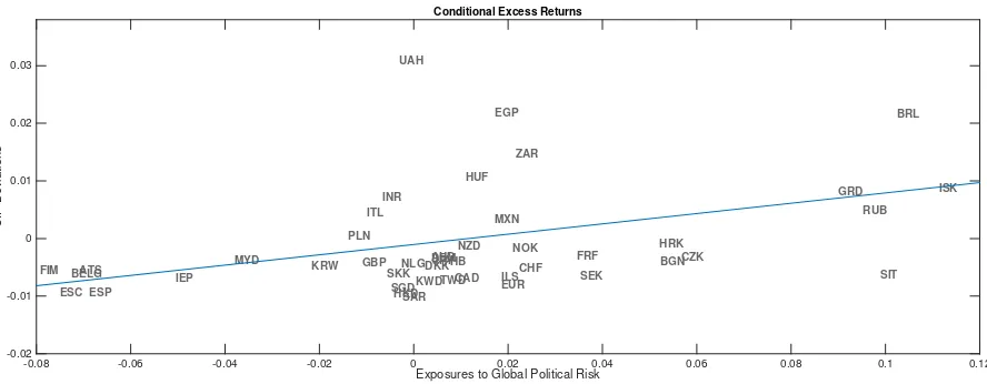
We also compute averagedeviations from the CIP condition after controlling for
transac-tion costs as another proxy of limits to arbitrage in the currency market (Mancini-Griffoli and
Ranaldo,2011). Figure2shows average CIP deviations along with global political risk betas
for conditional excess returns. We find that countries with high political risk exhibit more
pronounced CIP deviations, reflected in the positively sloped regression line, supporting our
hypothesis regarding the role of global political risk in currency momentum strategies. This
visual evidence is also verified by the significant estimated cross-sectional beta (β = 1.34,
tstat= 2.55) andR2 of 11%.
[Figure 2 about here.]
Global FX Volatility and Liquidity. We examine the behavior of political risk in
cur-rency momentum when we control for volatility or liquidity in the foreign exchange market.
We follow Menkhoff et al. (2012a) and measure FX volatility and liquidity based on the
cross-sectional average of individual daily absolute exchange rate returns that are averages
each month.39 As we did for the political risk measure, we compute the innovations ofAR(1)
38For examples on the construction of the idiosyncratic volatility and skewness please see Goyal and
Santa-Clara(2003);Fu(2009);Boyer, Mitton, and Vorkink(2009);Chen and Petkova(2012).
39We measure global FX volatility (σF X
t ) and FX liquidity (ξtF X) as: σF Xt = 1 Tt
P d∈Tt
h P
k∈Kd
|∆s
d|
Kd
i
andξtF X = T1t
P d∈Tt
h P
k∈Kd
BASk d
Kd
i
respectively, where|∆sd|represents the absolute change in the log
spot exchange rate of currency k on day d. In the same vein, BASk
d is the bid-ask spread in percentage
points of currency k on day d. Tt is the total number of days in month t and Kd is the total number of
models and denote them as ∆RVF Xt and ∆LF X
t respectively.
Global FX Correlation. Mueller, Stathopoulos, and Vedolin (2013) show that global
FX correlation is priced in the cross-section of carry trade portfolios and that it is a good
proxy for global risk aversion. It is very important to see the performance of political risk
under different states of correlation risk. We use a similar measure with the one introduced
by Mueller, Stathopoulos, and Vedolin (2013) and compute global FX correlation risk as:
γF X t =
1
Ncomb t
Pnt
i=1
h P
j>i RC ij t
i
, where RCtij is the realised correlation between currencies
i and j at time t. Ncomb
t is the total number of combinations of currencies (i, j) at time t
and nt is the total number of currencies in our sample at time t. As before, we replace the
correlation variable with its innovations from an AR(1) model and denote it ∆RCF Xt .
Double Sorts. We now turn our attention to the cross-sectional predictive ability of
po-litical risk conditional on the information encompassed in these variables. We compute the
exposure of conditional excess returns to political risk based on a 60-month rolling window
and then we sort conditional currency excess returns (i.e. momentum returns) first into two
portfolios based on the variable of interest and then, within each portfolio, we sort them
again into three bins based on global political risk exposures. Each portfolio is rebalanced
on a monthly basis. Note that we sort currencies into portfolios based on the currency
ex-posures to our variables with the exception of idiosyncratic volatility, where we use the raw
measure instead of its betas.40
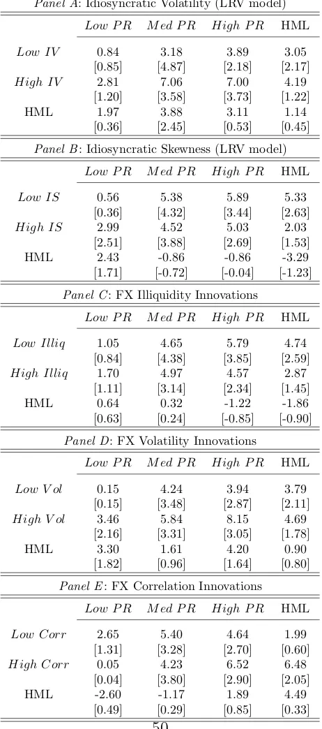
Starting with idiosyncratic volatility and skewness, Panels A and B of Table 7 show
results of the double sorts on IV ((idiosyncratic volatility) and IS ((idiosyncratic skewness),
respectively, along with global political risk exposures. Consistently with Menkhoff et al.
40We do not provide double sorts for CDS spreads because of data availability, i.e. short time-series and
(2012b), we find that momentum returns increase as we move from low to high IV portfolios
and also that the momentum returns are more extreme in the high idiosyncratic volatility
basket, making it more difficult for an investor to hedge this risk away. A reverse pattern
is observed for IS portfolios. We thus test whether this pattern influences our results. We
find that in both low and high IV portfolios, currencies with high political risk exhibit
higher mean excess returns than the low political risk counterpart, but the difference is more
pronounced in high IV portfolios. The results are similar for idiosyncratic skewness, except
that the difference across political risk portfolios is greater in low IS portfolios.
Another determinant of currency momentum is illiquidity. Menkhoff et al.(2012b) show
that currency momentum is more concentrated among countries with less liquid currencies
and a fragile political environment. We therefore need to examine the pricing ability of
political risk after controlling for illiquidity. Panel C of Table 7 shows that momentum
returns increase as we move from low to high political risk portfolios both in high and low
illiquidity states.
Another feature of exchange rates in relation to momentum portfolios concerns the level
of volatility. Thus, in Panel D we ask whether political risk is priced even after controlling
for global FX volatility. We find that momentum profitability is larger in high political risk
portfolios in comparison to low political risk baskets. This pattern is more striking in high
volatility states.
Finally, we control for global FX correlation in Panel D of Table 7so as to examine the
momentum profitability under high and low levels of globalrisk aversion. Here, we show that
the increasing pattern remains unchanged even after controlling for global FX correlation.
However, the difference across global political risk portfolios is particularly significant in low