Adaptive designs for complex dose finding studies

(1)

Adaptive Designs

for Complex Dose Finding Studies

by

Pavel Mozgunov

BA (Hons), Higher School of Economics, 2014

Submitted for the degree of

Doctor of Philosophy

at Lancaster University

(2)

Adaptive Designs for Complex Dose Finding Studies by Pavel Mozgunov, BA (Hons).

Submitted for the degree of Doctor of Philosophy at Lancaster University, April 2018

Abstract

The goal of an early phase clinical trial is to find the regimen (dose, combina-tion, schedule, etc.) satisfying particular toxicity or (and) efficacy characteristics. Designs for trials studying doses of a single cytotoxic drug are based on the funda-mental assumption “the more the better”, that is, the toxicity and efficacy increase with the dose. This monotonicity assumption can be violated for novel therapies and for more advanced trials studying drug combinations or schedules. It also be-comes common to consider a more complex endpoint rather than a binary one as they can carry more information about the drug. Both the violation of the mono-tonicity assumption and the complex outcomes give rise to important statistical challenges in designing novel clinical trials which require an extensive attention.

In the first part of this thesis, we consider a specific class of combination trials which involve novel therapies and can benefit from the monotonicity assumption. We also propose a general tool evaluating the performance of novel designs in the context of complex clinical trials. Further, we consider a problem of Bayesian inference on restricted parameter spaces. We propose novel loss functions for pa-rameters defined on the positive real line and on the interval demonstrating their performances in standard statistical problems. Based on the obtained results, we propose a novel allocation criterion for model-based designs that results in a more ethical allocation of patients.

(3)

(4)

(5)

Acknowledgements

I wish to thank two people without whom this work would not be possible: my supervisor, Prof Thomas Jaki, for providing a tremendous help and advice during my period of research and for broadening my mind; and my wife, Mrs Kristina Evtifeva, for the continuous support and inspiration. I would like to thank both of them for the endless patience in reading my manuscripts and in correcting my grammar.

I would also like to thank Dr Xavier Paoletti and Prof Mauro Gasparini for many useful discussions and for fruitful collaborations which resulted in several works upon which Chapter 2 and Chapter 3 are based, respectively.

I would like to thank Prof Mark Kelbert for introducing me to Information Theory and to its emerging area of weighted information measures which motivated the novel information gain criterion in Chapter 4.

(6)

Declaration

I declare that the work in this thesis has been done by myself and has not been submitted elsewhere for the award of any other degree.

The word count for this thesis is 49712 words.

Pavel Mozgunov

List of contributed papers

Section 2.2 has been submitted for publication as Mozgunov, P., Jaki, T. and Pao-letti, X. (2018) Randomized dose escalation designs for drug combination cancer trials with immunotherapy.

Section 2.3 has been submitted for publication as Mozgunov, P., Jaki, T. and Paoletti, X. (2018) A Benchmark for Dose Finding Studies with Continuous Out-comes.

The first part of Chapter 3 has been submitted for publication as Mozgunov, P., Jaki, T. and Gasparini, M. (2018) Loss Functions in Restricted Parameter Spaces and Their Bayesian Applications.

Section 3.5 has been submitted for publication as Mozgunov, P. and Jaki, T. (2018) Improving a safety of the Continual Reassessment Method via a modified allocation rule.

The first part of Chapter 4 has been submitted for publication as Mozgunov, P. and Jaki, T. (2018) An information-theoretic approach for selecting arms in clinical trials.

(7)

List of Tables

2.1 Operating characteristics of EmaxR, L2R, L2 and P1 models in scenarios 1-5 . . . 28 2.2 Operating characteristics of EmaxR, L2R, L2 and P1 models in

scenarios 6-9 . . . 29 2.3 Operating characteristics of EmaxR, L2R, L2 and P1 models:

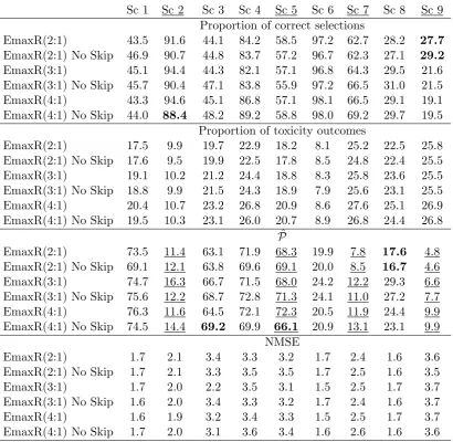
pro-portions of times the ET is found and NMSE. . . 31 2.4 Operating characteristics of EmaxR using different prior distributions. 35 2.5 Operating characteristics of EmaxR using different randomisation

ratios and no skipping constraint. . . 36 2.6 Complete information for 5 patients with randomly generated

toxi-city profiles. . . 40 2.7 Complete information for 5 patients with randomly generated

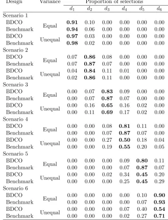
toxi-city and efficacy profiles. . . 44 2.8 Comparison of the BDCO design against the respective benchmark

in six scenarios. . . 47 2.9 Comparison of the BS design against the respective benchmark in

six scenarios. . . 49

3.1 Aggregated data of the Everolimus trial . . . 90 3.2 Values of the squared distance criterion used by CRM and of the

(12)

3.3 Proportions of each dose selections and mean proportions of DLTs for CRM, CIBP using a = {0.3,0.4,0.5}, and the non-parametric optimal benchmark. . . 94

4.1 Orderings for POCRM. . . 127 4.2 Operating characteristics of WE, CRM, POCRM and EWOC

de-signs in scenarios 1-3. . . 128 4.3 Operating characteristics of WE, CRM, POCRM and EWOC

de-signs in scenarios 4-6. . . 130 4.4 Operating characteristics of the WE design, MAB design and FR

in Trial 1. . . 133 4.5 Operating characteristics of the WE design, MAB design and FR

in Trial 2. . . 134 4.6 The range of considered regimens in the motivating trial. . . 136 4.7 Six permutations of scenario 1. . . 148 4.8 Mean number of toxicity and efficacy responses in scenarios 1−12

across six permutations. . . 155 4.9 Operating characteristics of WE (R) in scenarios 1-12: proportion

of optimal and correct rselections for different correlation values. . . 156

A.1 Proportions of dose selections and mean proportions of DLTs for CRM and the CIBP using the prior MTD d3 for the skeleton

con-struction. . . 165 A.2 Proportions of dose selections and mean proportions of DLTs for

CRM and the CIBP using the prior MTD d4 for the skeleton

con-struction. . . 166 A.3 Proportions of dose selections and mean proportions of DLTs for

CRM and the CIBP using the prior MTD d3 for the skeleton

con-struction and the novel criterion for the final selection. . . 167

(13)

B.2 Average computational time (min) for the exact algorithm and the simulations approach. . . 171 B.3 Operating characteristics of WE design in linear and unsafe

scenar-ios using different parameters of the safety constraint. . . 179

C.1 Proportion of optimal and correct dose selections in scenarios 1-8 and 13-14. . . 186 C.2 Mean number of toxicity and efficacy responses in scenarios 1−8

and 13−14. . . 187 C.3 Proportions of optimal dose selections, mean number of toxicity and

efficacy responses in scenarios 9-12. . . 188 C.4 Operating characteristics of WE, WE(R), RIV and WT designs in

scenarios 1-4. . . 189 C.5 Operating characteristics of WE, WE(R), RIV and WT designs in

scenarios 13-14. . . 192 C.8 Operating characteristics of WE in scenarios 1-12 with no early

(14)

List of Figures

2.1 Considered combination-toxicity scenarios. . . 25

2.2 Mean values and 95% credible intervals of toxicity probabilities for each combination using Emax, L2 and P1 models. . . 27

2.3 Mean values and 90% credible intervals of toxicity probabilities for each combination obtained by fitted EmaxR, L2R and L2 models in scenarios 1-4 . . . 32

2.4 Mean values and 90% credible intervals of toxicity probabilities for each combination obtained by fitted EmaxR, L2R and L2 models in scenarios 5-9. . . 34

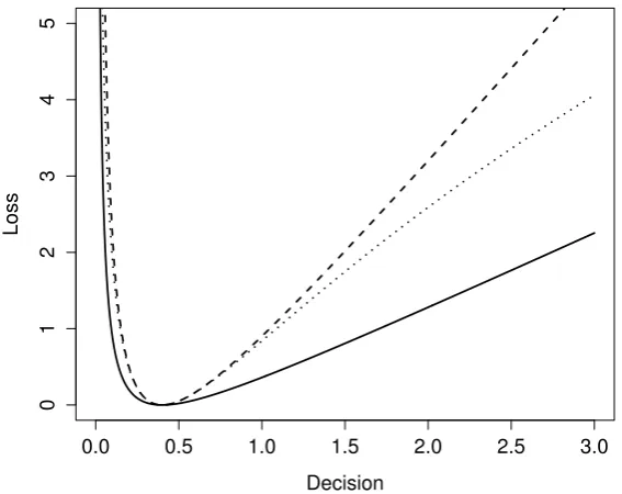
3.1 Examples of scale symmetric loss functions L1,Lsq, and D+. . . 62

3.2 Examples of the interval symmetric loss function (3.3.4). . . 68

3.3 Contour plots of loss functions D(2)₊ , L(2)₁ , L(2)sq. . . 72

3.4 MSE, variance and bias for the restricted estimator, the squared error loss function estimator and the Agresti-Coull estimator . . . . 74

3.5 Coverage probabilities using the normal approximation, Wilson method and delta-method. . . 76

3.6 MSE corresponding to different values of the restricted mean pa-rameter µand estimators U1, U2, U20, J. . . 79

3.7 Differences in MSEs for α1 andα2 using Bayes estimator under the squared error loss function and the Bayes estimator under L(2)sq. . . . 81

(15)

3.9 Values of the parameter of asymmetry a for γt = 0.20, γt = 0.25,

γt = 0.30 and ν∈(0,0.35). . . 88

3.10 Allocations of 7 cohorts in the individual Everolimus trial. . . 91

3.11 Six considered dose-toxicity scenarios for the comparison to the CRM. 92 3.12 Ten considered dose-toxicity scenarios for the comparison to EWOC. 96 3.13 Accuracy indexes and mean accuracy indexes for the non-parametric optimal benchmark, CIBP, TDFB, EWOC, TAR and BLRM designs. 97 3.14 Mean number of DLTs for CIBP, TDFB, EWOC, TAR and BLRM designs. . . 99

4.1 Weight function φn(p) ford= 2 and different values of κ. . . 109

4.2 Monotonic and non-monotonic toxicity scenarios. . . 125

4.3 ENS and power for WE design under Rule II and different κ. . . 133

4.4 Contours of the efficacy-toxicity trade-off function. . . 138

4.5 Allocation of 18 cohorts in the invididual trial. . . 144

4.6 Probabilities to allocate each of 18 cohorts to each regimen. . . 145

4.7 Eight plateau efficacy scenarios, four umbrella regimen-efficacy scenarios and two scenarios with no correct regimens. . . 149

4.8 Seven efficacy orderings. . . 152

4.9 Proportion of optimal and correct selections by WE(R) and WT designs in scenarios 1-12 across six permutations. . . 153

B.1 Expected number of observations at regimen 1 using different values of α1 obtained by the approximation and by simulations. . . 173

B.2 Operating characteristics of the approximation. . . 175

B.3 Proportion of correct selections by WE design using different values of β and step. . . 176

(16)

B.5 Geometric mean of proportions of correct selections by WE design using different values of β and step, and N = 25. . . 178

(17)

Chapter 1 Introduction

1.1 Background

Clinical trials are an integral part of drug development. A clinical trial is defined as a prospective study comparing effects of interventions in a human being. In the specific context of drug trials, four different phases of testing are conventionally identified (Friedman et al., 2015):

• Phase I, first in human clinical trials, primarily evaluating the basic safety of a drug

• Phase II, evaluating whether a drug has the desirable biological activity/activities

• Phase III, confirmatory trials, assessing the effectiveness of a drug and com-paring it to a standard of care or a placebo

• Phase IV, a post-marketing phase, which identifies and evaluates long-term effects of a drug

(18)

one or two dosing regimens that were found to be promising in terms of toxicity and efficacy during Phase I and Phase II clinical trials (Friedman et al., 2015). Therefore, successes in later phases depend, to a great extent, on the knowledge about the novel compound obtained in early phase clinical trials, which are argued to be one of the most important steps in the drug development. A well-designed early phase study is therefore essential to provide valuable information (Chevret, 2006). This underlines the need for effective statistical methods for the accurate selection of optimal dosing regimens. Early phase clinical trials are, however, con-ducted using a small number of patients or healthy volunteers and face particular ethical restrictions due to the limited knowledge about adverse events associated with a new drug. This raises many statistical challenges which need to be ad-dressed appropriately. Due to its great importance, the methodology for early phase clinical trials is a growing field and is attracting a lot of attention both from statisticians and clinicians (Chevret, 2006). In this thesis, we propose novel methods for early phase clinical trials prompted by emerging practical needs. The proposals in this thesis are mainly motivated by statistical challenges arising in the context of oncology studies. However, the majority of novel methodologies presented are generic and can be applied beyond cancer trials and beyond early phase designs.

(19)

Phase I clinical trials are the first studies in humans evaluating the toxicity of regimens. There is limited e affects a human body, and the initial step here is to find “safe” regimens. Given a discrete set of regimens, the goal of Phase I clinical trial is to identify the maximum tolerated regimen (MTR) defined as the regimen having the maximum acceptable level of toxicity γt (Friedman et al., 2015) wheretstands for toxicity andγtmight be a percentage, a score or a medical characteristic depending on the trial’s endpoint. Phase I clinical trials are usually referred to as regimen escalation trials. It is a common practice to summarise the data about the regimen’s toxic severity in a single binary outcome, a limiting toxicity, conventionally called dose-limiting toxicity, DLT, (Le Tourneau et al., 2009). In this case, γt is a maximum acceptable proportion of patients suffering toxicity. Then, the MTR defines the set of regimens that have an acceptable probability of DLT and can be studied in subsequent phases. We will use terms maximum tolerated dose (MTD) and maximum tolerated combination (MTC) in contexts of single agent and combination trials, respectively.

Once the set of safe regimens is defined, the second step is to ensure that at least one of them has a desirable therapeutic effect (Yin, 2013). To answer this question, the efficacy of regimens is evaluated in Phase II clinical trials. Given a discrete set of regimens, the goal of Phase II clinical trial is to find the regimen corresponding to a pre-specified efficacy level γe (where e stands for efficacy), which, again, can be a percentage, a score or a medical characteristic. Phase II clinical trials are usually referred asregimen ranging trials. Upon the completion of Phase II trials, the regimens (usually one or two) for a Phase III confirmatory clinical trial are selected (Friedman et al., 2015).

(20)

for both toxicity and efficacy endpoints and can result in a more reliable recom-mendation for Phase III study, particularly, for novel agents (Wages and Conaway, 2014). The goal of a Phase I/II clinical trial evaluating both toxicity and efficacy simultaneously is to find the optimal biologic regimen (OBR) corresponding to pre-specified levels of toxicity and efficacy.

Despite different formulations of research problems, the goals of all these trials are similar from the statistical perspective. The common goal of an early phase study is to find the regimen having characteristics “as close as possible” to the targetγ

which can be either a scalar (e.g. γt orγe) or a vector (e.g. (γt, γe)T). We would use the term target regimen (TR) to emphasise that a particular design can be applied to different types of trials.

1.2 Motivation

The primary motivation behind methods proposed in this thesis is the growing complexity of early phase clinical trials. It is becoming more common to con-sider more complex dosing regimens rather than doses of a single agent only. For instance, therapies using a combination of drugs have become the mainstream ap-proach to diseases such as cancer (Khalil et al., 2016) and tuberculosis (Kerantzas and Jacobs, 2017). It was found that administering several agents simultaneously can noticeably improve their safety profiles and therapeutic effects. However, po-tential synergistic (or antagonistic) effects give rise to additional challenges in designing early phase combination trials compared to single agent ones. A lot of

(21)

higher dose of the first compound, but a smaller dose of the second compound. In the vast majority of trials, clinicians cannot define which of these combinations is more toxic prior to the trial (Wages et al., 2011). The same argument holds when considering efficacy levels of combinations.

The schedule of administration can add an additional complexity as well (Kodama et al., 2009). As an illustration, consider a six days course of treatment and two dose-schedules: (i) 10 mg a day every day and (ii) 20 mg a day every two days. The total amount of drug received by a patient is the same by the end of six days, but it is unclear which of these dose-schedules is more toxic. A smaller dose is expected to reduce toxicity, but a more regular administration is expected to increase it. Again, clinicians cannot define which of these effects is greater in many clinical trials.

The problem of unknown ordering of toxicities and efficacies can also appear in the single agent context. While the paradigm “the more the better” holds for cytotoxic agents, it can be violated for molecularly targeted agents (MTA) which include hormone therapies, signal transduction inhibitors, gene expression mod-ulators, apoptosis inducers, angiogenesis inhibitors, immunotherapies, and toxin delivery molecules, among others. For MTAs either dose-efficacy or dose-toxicity relationships can have a plateau (Morgan et al., 2003; Postel-Vinay et al., 2011; Robert et al., 2014; Paoletti et al., 2014) or a dose-efficacy relationship can exhibit an umbrella shape (Conolly and Lutz, 2004; Lagarde et al., 2015).

(22)

the adequate identification of the TR are essential. In this work, we propose novel designs that are able to address either some or all of the stated challenges and extend several well-established early phase designs in order to guarantee a more accurate and ethical regimen selection.

1.3 Outline of Thesis

In Chapter 2 we consider several types of combination trials which can benefit from the monotonicity assumption. We show, however, that the straightforward appli-cation of standard Phase I dose escalation model-based designs may fail to address the goals specific to the combination context and propose an alternative. Further, we generalise the non-parametric optimal benchmark O’Quigley et al. (2002), a tool to evaluate the performance of regimen finding designs, to the setting of com-plex trials with multiple endpoints having discrete or continuous distributions.

In Chapter 3 we consider a problem of estimation in restricted parameter spaces that arise in many areas of regimen finding. We stress that standard criteria for the choice of estimators and for the allocation of patients might not be a proper choice in the context of early phase clinical trials. We demonstrate the performance of the proposed estimator in some classic statistical problems and construct a novel allocation criterion for a Phase I model-based design which improves its ethics.

In Chapter 4 the general setting of regimen finding clinical trials with the mono-tonicity assumption violation and multinomial outcomes is considered. We propose a class of novel designs which relax the monotonicity assumption and can be ap-plied in complex Phase I, Phase II and Phase I/II trials. We demonstrate their applications motivated by actual clinical trials.

(23)

Chapter 2 Model-based Dose Escalation

Designs and Optimal Benchmarks

2.1 Background

(24)

simple escalation/de-escalation rules which do not require any support from a statistician. The 3+3 design uses the information from the most recently enrolled patients only and ignores earlier data obtained in the trial. This results in a sys-tematic underestimation of the MTD, an unethical allocation of patients (patients are assigned to low doses far from the target toxicity) and a high risk of erroneous conclusions (Reiner et al., 1999). Instead, more statistical approaches that use all available information have been shown to lead to noticeable improvements in the probability of correct MTD selection (Wheeler, 2017). Below we recall the core of model-based dose escalation designs that formed the basis of many of regimen escalation methodologies.

2.1.1 Continual Reassessment Method Type Designs

Consider a single agent Phase I clinical trial with binary toxicity outcome, dose-limiting toxicity (DLT) or no DLT,N patients andmdose levelsd1, . . . , dm. LetYij be a binary (Bernoulli) random variable taking value yij = 0 if patient i has experienced no DLT given dosedj and yij = 1 otherwise. This random variable is characterised by toxicity probability pj such that pj = P(Yij = 1), i = 1, . . . , N. It is assumed that the toxicity probability is an increasing function of dose,p1 <

. . . < pm. The goal of the trial is to find the MTD, the dose corresponding to the target level of toxicity,γt.

(25)

Assume that toxicity probability pj has the functional form

pj =ψ(dj, θ) (2.1.1)

where θ ∈ _Rd _{is a} _d_{-dimensional vector of parameters and} _d

j is a scalar unit-less dose level (also refereed as standardised levels). Denote the prior distribution ofθ

byf0(·). Assume thatnpatients have been already assigned to dosesd(1), . . . , d(n)

and binary responsesy1, . . . , ynwere observed, respectively. The CRM updates the posterior distribution ofθ using Bayes’s Theorem

fn(θ) =

fn−1(θ)φ(d(n), yn, θ)

R

Rdfn−1(u)φ(d(n), yn, u)du

= f0(θ)

Qn

i=1φ(d(i), yi, θ)

R

Rdf0(u)

Qn

i=1φ(d(i), yi, u)du

(2.1.2)

where

φ(d(i), yi, θ) = ψ(d(i), θ)yi(1−ψ(d(i), θ))1−yi.

The posterior mean of the toxicity probability given dose dj after n patients is equal to

ˆ

p(_jn) =_E(ψ(dj, θ)|y1, . . . , yn) =

Z

Rd

ψ(dj, u)fn(u)du. (2.1.3)

Patients in the dose escalation trial are assigned cohort-by-cohort, where a cohort is a small group of typically 1 to 4 patients. Then, the dose dj that minimises

|pˆ(_jn)−γt|, (2.1.4)

or, equivalently, the squared distance pˆ(_jn)−γt

2

(26)

estimator (2.1.3).

There have been many developments building on the CRM since its original pro-posal. O’Quigley and Shen (1996) have considered a likelihood approach to CRM and Shen and O’Quigley (1996) have formulated the conditions of its consistency (the probability that the design would select the true MTD tends to 1 asN → ∞). Korn et al. (1994); Zohar and Chevret (2001); O’Quigley (2002) have consid-ered early stopping rules to accommodate practical challenges of implementations in actual clinical trials. Cheung and Chappell (2002); Lee and Cheung (2009); O’Quigley and Zohar (2010); Cheung (2011) have investigated choices of stan-dardised levelsd1, . . . , dm and parameters of the prior distributionf0. Cheung and

Chappell (2000) have proposed a modification called the time-to-event CRM which accommodates late-onset toxicities and leads to conducting a trial in a timely man-ner. Cheung (2005) has shown that the CRM does not lead to counter-intuitive escalation/de-escalation decisions that would not be accepted by clinicians. The CRM was subsequently extended to contexts of more complex trials, for example, to Phase I combination trials (Wages et al., 2011) and to Phase I/II dose finding trials (Braun, 2002).

While it is generally agreed that the Bayesian CRM design leads to an accurate MTD selection, the choice ofψ(dj, θ) is debated (Iasonos et al., 2016). The common parametric forms of the model function are given below.

Choice of the Working Model in Model-based Designs The common choice for the 1-parameter working dose-toxicity model is

ψ(dj, θ) =d

exp(θ)

j (2.1.5)

(27)

On the other hand, it is argued that the 1-parameter model (2.1.5) does not re-flect the anticipated dose-toxicity relation (Neuenschwander et al., 2008). Instead, the logistic function was suggested as an appropriate alternative with a clinically relevant interpretation. Whitehead and Williamson (1998) proposed to use the 2-parameter logistic model

ψ(dj, θ1, θ2) =

exp(log(θ1) +θ2dj)

1 + exp(log(θ1) +θ2dj)

(2.1.6)

where θ1, θ2 are scalar parameters. There are variants of the logistic model: with

parameterθ1 being known and fixed and with bothθ1 andθ2 being unknown. The

same parametric model was also used by Babb et al. (1998). This model is seen to be appropriate in the context of actual clinical trials and is extensively employed in practice (Neuenschwander et al., 2008) despite potential inconsistency problems raised by Iasonos et al. (2016). Paoletti and Kramar (2009) have compared several model choices of ψ(·) in a comprehensive simulation study. Routinely, models with more than two parameters are not routinely considered in the setting of dose escalation trials.

(28)

2.1.2 An Optimal Benchmark for Studies with a Binary

Endpoint

A variety of dose finding methods for Phase I clinical trials aiming to find the MTD were developed in the literature since the proposal of the CRM. A conventional way to assess the performance of a design is to conduct an extensive simulation study. One of the key characteristics of any regimen finding method is its accuracy which is usually computed as the proportion of times the true target regimen (e.g. the MTD) is selected (also referred as the proportion of correct selections - PCS). The majority of novel proposals are studied in scenarios chosen by investigators themselves. This, clearly, adds subjectivity to the assessment of a method’s oper-ating characteristics as one can always find scenarios in which the TR selection is easier than in others.

To solve this problem, O’Quigley et al. (2002) proposed the non-parametric opti-mal benchmark that provides an upper limit of accuracy (in terms of the PCS) for dose finding methods based on a binary toxicity endpoint. The benchmark uses the complete information concept which assumes that outcomes of each patient can be observed at all dose levels (in contrast to an actual trial in which a pa-tient can be assigned to one dose only). The benchmark shows how “difficult” the TR identification is in the chosen scenario and provides the objective context for the performance evaluation of the design under investigation. Since its proposal, the benchmark has proven its great usefulness to assess newly proposed designs comprehensively (see e.g. Paoletti and Kramar, 2009; Yin and Yuan, 2009). Ad-ditionally, based on the benchmark, Cheung (2013) derived sample size formulae for the CRM.

(29)

thatp1, . . . , pm are known. In other words, for a given patient one knows the max-imum toxicity probability that this patient can tolerate. Formally, the information about the response of patient i at all dose levels is summarised in a single value

ui ∈ (0,1), profile of the patient, which is drawn from a uniform distribution,

U(0,1). The value ui was also defined as a tolerance of patienti by Finney (1952) who, historically, was one of the originators of the idea of having an increasing series of probabilities generated by shareholding a continuous distribution which formed a basis for the complete information concept. For instance,ui = 0.3 means that patient i can tolerate doses dj with pj ≤ 0.3, but would experience a DLT if given dose dj0 with pj0 > 0.3. It follows that ui is transformed to yij = 0 for doses with pj < 0.3 and to yij = 1 otherwise. The procedure is repeated for N patients which results in the vector of responses corresponding to each dose level

y_j = (y1j, . . . , yN j),j = 1, . . . , m. LetT(yj, γt) be a summary statistic for the dose level dj upon which the decision about the MTD selection is based. Convention-ally,T(y_j, γt) is chosen such that its minimum (or maximum) value corresponds to the estimated MTD. Therefore,dj for which T(yj, γt) is minimised (maximised) is selected as the MTD in a single trial. The procedure is repeated for S simulated trials and then proportions of each dose selections are computed.

In a context of Phase I clinical trial with a binary endpoint

T(y_j, γt) =

PN

i=1yij

N −γt

(2.1.7)

is a conventional choice for the MTD selection criterion. Wages and Varhegyi (2017) proposed a Web application for the benchmark evaluation using this crite-rion.

(30)

Cheung (2014) generalized the benchmark to both of these cases. This has broad-ened the benchmark application significantly. However, there are a growing num-ber of Phase I and Phase I/II clinical trials involving continuous endpoints, but no corresponding benchmark exists. For example, Bekele and Thall (2004); Yuan et al. (2007); Ivanova and Kim (2009); Bekele et al. (2010); Ezzalfani et al. (2013); Wang and Ivanova (2015) considered a continuous toxicity endpoint while, for ex-ample, Bekele and Shen (2005); Hirakawa (2012); Yeung et al. (2015, 2017) studied Phase I/II trials with binary toxicities and continuous efficacies.

In Section 2.3, we propose a new benchmark which can be applied to dose find-ing studies with continuous outcomes and shares the same concept of the com-plete information as the original approach. We demonstrate the application of the benchmark in contexts of recently proposed Phase I and Phase I/II dose finding designs.

2.2 Designs for Combination Trials Involving

an Immunotherapy

2.2.1 Problem Formulation

(31)

combination trials investigating either (i) the added value of an immune checkpoint blocker to a backbone therapy or (ii) the added value of a new agent to an immune checkpoint blocker (Pardoll, 2012). In both cases, one agent, called a standard of care, is administered at a fixed dose and another agent is dose-escalated. While such setting allows for the straightforward adaptation of single agent designs, it also hides potential difficulties.

The conventional goal of Phase I drug combination trial is to find the maximum tolerated combination (MTC). However, many studies of immunotherapies have never actually reached the maximum tolerated level as stated above. An im-munotherapy can also have a complex mechanism of its interactions with other compounds (Sharma and Allison, 2015). Consequently, when considering combi-nation trials involving an immunotherapy, the information beyond the conventional (and only) objective of a Phase I study can be also important for a more accurate choice of the combination(s) to study in subsequent phases.

We focus on the setting that covers two important types of Phase I clinical trials with corresponding research questions added to the MTC selection:

1. The standard of care is a toxic agent (e.g. chemotherapy) and is given at the full (single agent) dose and an immune-checkpoint blocker is dose-escalated.

A clinician would tolerate only a slight increase τ in the toxicity of combi-nation compared to the toxicity of the standard of care (Paller et al., 2014) and the question whether “the increase in toxicities is acceptable?” should be tested.

2. The standard of care corresponds to a low toxicity level (e.g. an immune-checkpoint blocker) and is given at the full (single agent) dose and either a toxic agent or an MTA is dose-escalated.

(32)

and the standard of care which would help to define the therapeutic index (a ratio of the dose that produces highest acceptable toxicity to the dose needed to produce the desired therapeutic response) more accurately. A plateau is defined by not exceeding the difference in associated toxicities by more than τ.

(b) A clinician has an expectation of an additional toxicity τ over the stan-dard of care under the assumption of compounds independence. An interest lies in checking for an interaction effect defined as an additional toxicity over τ.

The objectives of these trials are (i) to identify the MTC, (ii) to quantify the ex-pected difference between single and combination treatments and (iii) to determine the shape of the dose-toxicity relationship. These clinical trials share a common interest in the comparison of toxicity levels associated with the estimated MTC and the standard of care alone but they differ in their motivation. To unify nota-tion, we study the extra toxicity (ET) beyond the expected differenceτ. We show that standard single agent dose-escalation methods currently used for such trials may fail to address secondary questions of the trial.

To achieve all objectives, we suggest to adapt two modifications to the Bayesian model-based design. We propose to include the standard of care given alone as a control arm and, to randomise each patient to the control arm or to the combi-nation selected by the Bayesian model-based design. We demonstrate that such randomisation procedure leads to a reliable statistical evaluation of the ET (added over the standard of care) and of the general interaction effects between com-pounds. We also show that the Emax model provides a well-established tool to detect and to evaluate different patterns in the dose-toxicity relationship and its parameters match the information needed to address stated objectives.

(33)

trials is widely debated in the literature (e.g. Saad et al., 2017). The main argu-ment against is the monotonicity assumption that makes comparing toxicity levels unnecessary and results in considering the control group as not contributing to the goal of the trial (the MTC selection). However, this assumption has been found to be inappropriate for many immunotherapies. Importantly, patients allocated to the control arm receives the standard of care which makes the randomisation an ethically viable option. It will be also demonstrated that modelling the data observed for the control group simultaneously with the escalated arm contributes to toxicity estimates for all dose levels and can serve the MTC selection objective as well.

2.2.2 Motivating Trials

The proposed design is motivated by two recent combination trials that could potentially benefit from its implementation.

Gemcitabine is a standard chemotherapy for an advanced pancreatic cancer (Agli-etta et al., 2014) which has a narrow therapeutic index (Crane et al., 2002). Treme-limumab is a fully humanized monoclonal antibody against CTLA-4 that may al-low effective immune responses against tumour cells. In several clinical studies, anti-CTLA4 agents have been shown to induce durable tumour responses through modulation of the immune system in patients with metastatic melanoma (Buch-binder and Desai, 2016). The hypothesis was that the combination of these two agents “might provide a synergistic anti-tumour activity without increasing tox-icity” (Aglietta et al., 2014). Gemcitabine 1000 mg/m2 _{was administered in all}

(34)

Finally, the highest dose was recommended for further investigations, but the ques-tion whether the toxicity is increased over a clinically meaningful difference τ was never formally tested.

Sorafenib is a treatment for advanced cellular cell carcinoma. However, its efficacy remains limited as the time to progression is around six months. Despite this agent is being prescribed at the MTD (800mg/kg), its therapeutic index makes it possible to reduce the dose in case of adverse reactions (Wilhelm et al., 2006). SPLASH is a dose-escalation study of Avelumab in combination with sorafenib in patients with advanced cellular cell carcinoma that is about to be initiated at the Hospital Gustave Roussy. While Avelumab will be given at a fixed dose, Sorafenib will be escalated from 200 mg/kg up to 800mg/kg. The MTD is defined as the highest dose having the probability of DLT during cycle 1 closest to 25%. The expected DLT probability for Avelumab alone is 8%.

2.2.3 Randomisation and Emax Model

Framework Consider a clinical trial in which combinations of agentsA andB

are studied. The drug A is a standard of care given at the fixed dose, a, and B

is dose-escalated. We specify increasing doses ofB: 0 = b0 < b1 < b2 < . . . < bm. Then, ˜d0 ={a, b0},d˜1 ={a, b1}, . . . ,d˜m ={a, bm}arem+1 combinations available in the trial, where ˜d0 corresponds to the agent A given as a single agent and is

subsequently referred to as the control arm, and the combinations ˜d1, . . . ,d˜m are referred to as theinvestigational arms. A clinician observes binary outcomes, DLT and no DLT. Let pj be the probability for a patient to experience a DLT given the combination ˜dj. It is assumed that toxicity is a non-decreasing function of combination, p0 ≤ p1 ≤ . . . ≤ pm and reliable prior information for the toxicity probability of the control arm, p0, is available.

(35)

the dose-escalation clinical trial is to find the MTC ˜dj? such that

j? = argmin j=0,...,m

|pj −γt|

using estimated toxicity probabilities ˆp0, . . . ,pˆm. The secondary goal, specific to combination trials, is to test if the difference of toxicity probabilities associated with the estimated MTC and the standard of care is as expected. The ET is defined in terms of the expected difference, τ. One would conclude the ET when the probability that the difference in the two estimated risks of toxicity exceedsτ

is larger than some credible level α. Formally, if the ET is present one would like the probability

P ≡_P(_P(ˆpj?−pˆ₀ ≥τ)> α) (2.2.1)

to be equal to 1. In contrast, if there is no ET, the probability (2.2.1) is desired to be equal to 0.

Note that as only one drug is varied, the problem can be considered as a uni-dimensional MTC search and the CRM (Section 2.1.1) can be applied. It, however, is designed for the MTC selection only, therefore, we introduce two design features into it.

Randomisation between control and investigational arms Patients in dose-escalation trials are assigned cohort-by-cohort. According to the original al-location rule, the CRM design tends to assign the majority of patients in the neighbourhood of the MTC. This leads to a sparse allocation of patients on other combinations and on the control arm. This will make it difficult to test for dif-ferences in toxicity risk associated with the estimated MTC and the control arm. We introduce the following randomisation procedure between the investigational (combinations) and control (standard of care) arms.

(36)

assigned to the estimated MTC by CRM according to the criterion (2.1.4), andc2

be the number of patients in cohort assigned to the control arm, ˜d0. This results

in at least N2 = _cc2

1+c2N patients on the control arm and at mostN1 =

c1

c1+c2N on

the investigational arm by the end of the trial. For instance, taking c1 = 3 and

c2 = 1 (denoted by 3:1), one will end up with at least 25% of the total sample

size being assigned to the control. Note that the model-based design is allowed to select the control arm as the estimated MTC if the associated toxicity is the closest to the targetγt. This facilitates avoiding exposing patients to high toxicity if the first combination has an unacceptable DLT probability. Therefore, the total number of patients on the control arm can be more than c2

c1+c2N.

Importantly, in the proposed design the values of c1 and c2 are fixed before the

trial. While the choice of these values is investigated in Section 2.2.6, their choice can be also guided by a prior information that a clinician has about the standard of care. For example, if a clinician is certain about the toxicity risk associated with the standard of care, one can allocate more patients to the investigational arms and use lower value ofc2.

The modified allocation rule (the randomisation of patients between control and investigational arm) raises an important question of the suitable choice of the parametric model ψ(dj, θ) which is discussed below.

4-parameter Emax model In the context of the single agent trial, the 1-parameter power model is argued to be an appropriate choice (Iasonos et al., 2016). There are, however, at least two reasons why 1-parameter models are not suitable for the type of trials considered here.

(37)

considered combination trials.

Secondly, one of the main arguments behind using a 1-parameter model (and, consequently, the main critique of models with more parameters) is that the CRM design tends to collect observations in the neighbourhood of the MTC only. This means that the approximation of the dose-toxicity relation is of interest in the neighbourhood of one point only. Clearly, 1-parameter models are rich enough to achieve it. Note, however, that given the randomisation step proposed above, the majority of patients will be now assigned in the neighbourhood of two points: the control arm and the estimated MTC. Therefore, more flexible models are essential to consider.

Motivated by the ability to model a plateau in a combination-toxicity relation, we propose to use the 4-parameter Emax model

ψ(dj, E0, Emax, λ, ED50) =E0+

dλ_jEmax

dλ

j +ED50λ

,

where E0 is the toxicity probability associated with the control arm, Emax+E0

is the maximum toxicity probability attributable to the combination,ED50 is the

combination which producesE0+Emax₂ toxicity andλis the slope factor. Following

the assumption of the non-decreasing toxicity probability, we specify λ ≥ 0. To adjust the single agent model to the combination setting, the unit-less variabledj, corresponding to the same toxicity probability as the combination ˜dj, is used. To construct dj one needs to represent them in terms of prior estimates of toxicity probabilities ˆp(0)_j associated with combinations ˜dj j = 0, . . . , m

dj = ˆED

(0) 50 ×

ˆ

p(0)_j −Eˆ₀(0)

ˆ

Emax(0) + ˆE₀(0)−pˆ(0)_j

!_ˆ1

λ(0)

where ˆλ(0), ˆE₀(0), ˆEmax(0) and EDˆ

(0)

50 are point prior estimates of model parameters.

(38)

Therefore, by definition, ˆp0(0) ≡Eˆ (0)

0 that leads to d0 = 0. Modelling E0 directly

guarantees that the sequential update of other parameters does not contribute to the toxicity probability estimation on the control arm. In this case, the model takes the trivial form

ψ(d0,·) = E0.

Intuitively, it reflects that the toxicity probability of the standard therapy does not depend on the mechanism of its interaction with compound B.

The parameters of the Emax model allows to model the toxicity on the control arm and the plateau. Modelling a plateauing dose-toxicity relationship (e.g. im-munotherapies) is not possible with other working models, e.g. two-parameter logistic form. We investigate the choice of the parametric model in the numerical study below.

2.2.4 Simulation Setting

We explore the performance of the Bayesian model-based dose-escalation method incorporating randomisation to the control arm into the Emax model by simu-lations in different scenarios. Motivated by a recent combination trials review by Riviere et al. (2015) we consider a setting with N = 48 patients and m = 7 combinations. We set the target toxicity probability γt = 0.25, the expected dif-ference τ = 0.05 and the confidence level α= 0.90.

Three main characteristics, (i) the proportion of correct selections (PCS), (ii) the proportion of times the ET is concluded and (iii) a goodness-of-fit measure, are considered. A goodness-of-fit measure is used to capture the overall shape of the dose-toxicity relationship. We use the scenario-normalized mean squared error (NMSE) defined as

N M SE= 1

S

X

s=1

v u u t

Pm

j=0(pj −pˆ (s)

j )2

Pm

j=0(pj−pˆoptj )2

(39)

where S is the number of replications, ˆp(_js) is the toxicity probability estimate for combination ˜dj obtained by the design in sth simulation and ˆp

opt

j is the toxicity probability estimate for combination ˜dj obtained by the non-parametric optimal benchmark approach described in Section 2.1.2. The normalisation facilitates com-parisons betwen different scenarios as the optimal benchmark incorporates their specificities. The value of the NMSE being equal to 1 corresponds to the curve estimated as precise as by the optimal benchmark.

Prior Specification The standardised levels, dj, are constructed using the skeleton ˆp(0).

ˆ

p(0) = [0.08,0.25,0.35,0.45,0.55,0.65,0.70,0.75]T.

The first value, 0.08, corresponds to the mean prior toxicity probability for the control arm. The prior MTC being the first combination ensures that the trial is started at the lowest combination. Other values are obtained by taking an adequate spacing between prior values. It has been shown by O’Quigley and Zohar (2010) that the CRM design is robust and efficient in this case. In contrast to the skeleton that is the same regardless which parameter model is used, the prior distributions of the model parameters needs to be calibrated such that all competing designs carry the same amount of the prior information.

To ensure that the proposed approach and competitive designs are evaluated un-der comparable set-ups the credible intervals for the prior toxicity probabilities associated with the control arm and the prior MTC are used. Taking into account that one usually has a reliable information about the standard therapy, but lim-ited information about combinations, we specify prior distributions to satisfy the following conditions:

1. The control arm ˜d0: the expected toxicity probability is ˆp (0)

0 = 0.08 and the

(40)

2. The prior MTC ˜d1: the expected toxicity probability is ˆp (0)

1 = 0.25 and the

upper bound of the 95% credibility interval is 0.80.

Following these conditions the prior distributions of the Emax model parameters are specify as

E0 ∼B(0.8,10−0.8), Emax|E0 ∼U[0,1−E0], ED50∼Γ(0.4,0.4), λ∼Γ(1,1)

(2.2.3) where _B(u, v) denotes the Beta distribution with parameters u, v and Γ(u, v) de-notes the Gamma distribution with the mean u_v and the variance _vu2. As the

choice of prior distributions may have quite a significant impact on the estimates of parameters, we first rely on the elicitation given in Equation (2.2.3), but also investigate the robustness to different prior distributions in Section 2.2.6. We refer to the design using the Emax model with proposed randomisation as “EmaxR”.

Cohort Size for the Control Arm and Combination Skipping The co-hort size is fixed to be c1 = 3 for the investigational arm and c2 = 1 for the

control arm. Therefore, at least 12 patients (25% of the total sample size) will be allocated to the standard therapy and at most 36 patients are allocated to the investigational arm. We allow combinations to be skipped. Other randomisation ratios, 2 : 1 and 4 : 1, and an impact of no skipping constraint are studied in Section 2.2.6.

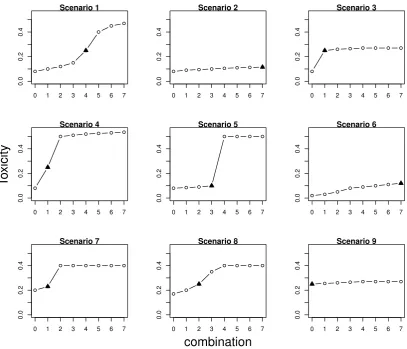
Scenarios Nine qualitatively different scenarios, depicted in Figure 2.1, are used to study the performance of the proposed approach. Scenarios 1-5 are con-sistent with the prior information about the control arm. Scenario 1 corresponds to a commonly used logistic dose-toxicity shape while scenario 2 considers a flat dose-toxicity curve with the MTC being ˜d7 and no ET beyond τ. In scenario 2,

the model monotonicity assumption implies that the toxicity probability on the control has the largest difference with combination ˜d7 and the model is expected

(41)

ran-0 1 2 3 4 5 6 7

0.0

0.2

0.4

Scenario 1

0 1 2 3 4 5 6 7

0.0

0.2

0.4

Scenario 2

0 1 2 3 4 5 6 7

0.0

0.2

0.4

Scenario 3

0 1 2 3 4 5 6 7

0.0 0.2 0.4 Scenario 4 T o xicity

0 1 2 3 4 5 6 7

0.0

0.2

0.4

Scenario 5

0 1 2 3 4 5 6 7

0.0

0.2

0.4

Scenario 6

0 1 2 3 4 5 6 7

0.0

0.2

0.4

Scenario 7

0 1 2 3 4 5 6 7

0.0

0.2

0.4

Scenario 8

combination

0 1 2 3 4 5 6 7

0.0

0.2

0.4

[image:41.595.113.521.67.416.2]

Scenario 9

Figure 2.1: Considered combination-toxicity scenarios. The MTC is marked by a triangle.

domisation to the control arm together with the Emax model can prevent false conclusions regarding the ET. Scenarios 3-4 correspond to steep dose-toxicity re-lationships that have a plateau around and outside the target toxicity probability, respectively. These scenarios are used to investigate under what conditions it is easier to find the ET. Scenario 5 also corresponds to a sharp increase in toxicities, but for medium combinations having unacceptably high toxicity such that there is no ET between the MTC and the control arm.

Scenario 6 reflects the case of a misspecified prior toxicity probability for the control arm - the true toxicity probability for ˜d0 is below the prior value. The

(42)

probability for the control is underestimated by the prior information and the control arm has a toxicity probability close to the maximum acceptable one. Both cases with (scenario 8) and without (scenarios 7, 9) ET are considered.

Competing Models The performance of the proposed approach is compared to designs that are currently used for the considered types of trials: the 1-parameter power model

pj(dj, θ) =dθj

denoted by P1 and the 2-parameter logistic model given in Equation (2.1.6) with-out randomisation denoted by L2. We also explore the possibility of randomisation to the control arm using the 2-parameter logistic model denoted by L2R. As there are only at most 36 patients on the investigational arm in the randomised setting against 48 in the non-randomised one, we also consider the 2-parameter logistic model without randomization and N = 36. This would allow spotting the influ-ence of the randomisation on the operating characteristics. Prior distributions for the parameters of P1 and L2, L2R modelsθ ∼Γ (5.5,3) and

(log(θ1),log(θ2))T ∼ N



 

log

0.08 0.92

−0.75,0.675

T

,



 

1.5 0 0 0.75



 



 

are chosen to satisfy approximately two conditions on prior distribution of ˜d0

and ˜d1 formulated above. While these prior parameters are chosen to satisfy

condition on two combination only, the difference can be found for the rest of combinations. Figure 2.2 shows the prior distributions of the toxicity probability on each combination imposed by the specified parameters’ prior distributions for Emax, L2 and P1 models.

As expected the prior distributions of the toxicity probability associated with combinations ˜d0 and ˜d1 have similar characteristics for all models. At the same

(43)

0 1 2 3 4 5 6 7

0.0

0.2

0.4

0.6

0.8

1.0

Emax

Combination

Pr

ior T

o

xicity

0 1 2 3 4 5 6 7

0.0

0.2

0.4

0.6

0.8

1.0

L2

Combination

0 1 2 3 4 5 6 7

0.0

0.2

0.4

0.6

0.8

1.0

P1

Combination

Figure 2.2: Mean values (black circles) and 95% credible intervals (dashed lines) of toxicity probabilities for each combination using Emax, L2 and P1 models.

more flexible models allow for a more informative prior distribution of the toxicity probability associated with the standard of care while leaving the distributions of the rest of combinations vague. At the same time, the prior by P1 cannot achieve the same as one parameter is used only and the distribution of the toxicity probability associated with the standard of care cannot be imposed independently of the other combinations.

The characteristics of all models compared are evaluated in R (R Core Team, 2015) using the bcrm-package by Sweeting et al. (2013). To accommodate the randomisation to the control arm and the Emax model corresponding modifications to the package were made. For all methods 104 _{replicated trials were used. The}

posterior distribution of parameters were found using JAGS (Hornik et al., 2003). The number of burn-in iterations is 2000, the number of production iterations is 104 and two chains were used.

2.2.5 Operating Characteristics

(44)

[image:44.595.115.517.131.628.2]

Table 2.1: Operating characteristics of EmaxR, L2R, L2 and P1 models in sce-narios 1-5: proportions of each combination selections and mean proportions of toxicity outcomes (DLTs). The MTC selection is in bold. Results are based on 104 _{replications.}

˜

d0 d˜1 d˜2 d˜3 d˜4 d˜5 d˜6 d˜7 DLTs

Scenario 1

Toxicity 0.08 0.10 0.12 0.15 0.25 0.40 0.45 0.47

EmaxR 0.0 2.1 8.8 24.9 43.1 13.6 3.8 3.7 19.1

L2R 0.0 1.8 8.3 26.5 44.6 13.8 3.1 2.0 19.2

L2(N = 36) 0.4 0.6 4.4 29.7 45.4 15.6 2.4 1.5 25.2

L2 0.4 0.1 3.5 24.9 52.6 16.4 2.1 1.3 25.1

P1 0.0 1.0 4.2 16.5 51.4 20.4 5.5 1.0 29.2

Scenario 2

Toxicity 0.080 0.090 0.095 0.100 0.105 0.110 0.112 0.115

EmaxR 0.0 0.3 0.5 0.9 0.5 1.6 1.9 94.4 10.2

L2R 0.0 0.6 0.8 1.5 1.8 1.6 2.5 91.2 10.1

L2(N = 36) 0.1 0.3 0.8 0.3 0.9 1.1 2.0 94.5 11.0

L2 0.3 0.1 0.3 0.5 1.8 1.0 0.5 95.6 11.4

P1 0.0 0.0 0.0 0.0 0.0 0.6 0.8 98.7 11.3

Scenario 3

Toxicity 0.08 0.25 0.26 0.265 0.27 0.27 0.27 0.27

EmaxR 2.4 44.3 13.9 7.3 7.1 5.0 4.1 15.9 21.2

L2R 2.8 44.7 15.8 10.1 7.6 4.4 2.5 12.1 21.3

L2(N = 36) 5.3 25.5 13.4 10.1 10.6 7.53 5.7 21.9 25.3

L2 5.1 27.0 13.0 9.4 11.5 7.1 6.1 20.7 25.3

P1 0.0 0.0 0.5 0.5 13.4 18.9 17.9 44.7 26.6

Scenario 4

Toxicity 0.080 0.250 0.500 0.510 0.520 0.525 0.530 0.535

EmaxR 5.1 82.1 11.5 0.9 0.3 0.1 0.0 0.0 24.4

L2R 4.1 86.4 8.4 0.9 0.3 0.0 0.0 0.0 24.6

L2(N = 36) 20.7 72.0 6.1 0.7 0.3 0.1 0.0 0.0 28.4

L2 20.9 75.0 4.0 0.1 0.0 0.0 0.0 0.0 26.9

P1 20.2 71.7 7.4 0.7 0.0 0.0 0.0 0.0 31.0

Scenario 5

Toxicity 0.080 0.085 0.090 0.100 0.50 0.50 0.50 0.50

EmaxR 0.0 1.9 7.8 57.1 31.2 1.6 0.1 0.4 18.8

L2R 0.0 1.5 9.5 56.4 30.2 1.4 0.8 0.3 18.2

L2(N = 36) 0.0 0.0 4.1 59.7 31.7 1.5 0.5 0.4 26.1

L2 0.1 0.1 1.4 62.7 35.5 0.2 0.1 0.0 25.1

P1 0.0 0.0 0.0 54.9 36.4 7.0 1.2 0.5 33.2

(45)

[image:45.595.116.517.131.533.2]

Table 2.2: Operating characteristics of EmaxR, L2R, L2 and P1 models in sce-narios 6-9: proportions of each combination selections and mean proportions of toxicity outcomes (DLTs). The MTC selection is in bold. Results are based on 104 _{replications.}

˜

d0 d˜1 d˜2 d˜3 d˜4 d˜5 d˜6 d˜7 DLTs

Scenario 6

Toxicity 0.020 0.030 0.050 0.080 0.090 0.100 0.110 0.115

EmaxR 0.0 0.0 0.0 0.0 0.4 1.1 1.2 97.2 8.3

L2R 0.0 0.0 0.0 0.0 1.0 1.1 1.9 96.1 8.7

L2(N = 36) 0.0 0.0 0.0 0.0 0.6 0.9 0.8 97.5 10.9

L2 0.0 0.0 0.0 0.1 0.1 0.2 0.5 99.3 11.3

P1 0.0 0.0 0.0 0.0 0.0 0.1 1.1 98.8 11.3

Scenario 7

Toxicity 0.20 0.23 0.40 0.40 0.40 0.40 0.40 0.40

EmaxR 12.7 64.3 15.1 4.7 1.7 0.7 0.5 0.4 25.8

L2R 9.4 67.2 15.7 5.3 1.4 0.3 0.4 0.3 25.8

L2(N = 36) 19.0 52.0 18.3 4.5 2.0 1.7 1.4 1.1 30.1

L2 15.0 62.5 15.1 3.6 1.8 0.8 0.8 0.5 29.2

P1 0.2 28.0 29.2 23.5 14.1 3.87 0.8 0.4 35.2

Scenario 8

Toxicity 0.17 0.20 0.25 0.35 0.40 0.40 0.40 0.40

EmaxR 5.1 40.3 29.5 16.1 5.9 1.7 0.8 0.5 23.6

L2R 2.8 45.3 31.5 12.7 4.9 1.8 0.8 0.20 23.3

L2(N = 36) 4.5 27.5 34.3 19.1 7.3 3.1 1.5 2.7 29.0

L2 4.5 24.9 41.1 19.1 6.5 1.9 1.1 0.9 28.6

P1 0.0 3.4 30.2 37.5 18.7 7.27 1.7 1.1 32.3

Scenario 9

Toxicity 0.25 0.255 0.26 0.265 0.27 0.27 0.27 0.27

EmaxR 21.6 37.6 10.0 7.9 4.7 4.3 2.3 11.6 25.5

L2R 19.6 43.3 12.9 7.2 5.2 2.4 2.1 7.3 26.1

L2(N = 36) 10.1 20.7 12.5 10.5 10.1 6.3 5.8 24.0 26.0

L2 10.1 22.9 12.7 10.3 9.5 8.0 6.4 20.0 26.3

P1 0.3 6.5 15.0 26.7 28.1 12.8 6.9 3.7 26.6

(46)

36). Note that the misspecified prior distribution for the control arm (scenarios 6-9) does not affect the MTC selection noticeably. Note that the inclusion of randomisation to the control leads to decrease the proportion of toxicity outcomes almost in all scenarios. For instance, it is decreased by up to 6% in scenario 1 that results in nearly two fewer patients experienced adverse events. The decrease in number of DLTs in the approaches with randomisation can be explained by the fact that the standard of care ˜d0 has the lowest DLT probability and at least 25%

of patients are allocated to it. At the same time, the design without randomisation tends to allocate the majority of patient to the investigational arms having greater probabilities of toxicity.

In scenarios 2 and 6, the MTC is the highest combination and all models select it correctly in more than 90% of replications with L2R having the least PCS: 91.2% in scenario 2 and 96.1% in scenario 6. In scenario 9 where the control arm is already associated with the maximum acceptable toxicity, the randomised designs select the control arm by nearly 10% more often than L2. Generally, the randomised designs select combinations in the beginning of the curve ( ˜d1−d˜3) more often with

nearly 70% of ˜d0,d˜1,d˜2 selections against 45% for L2 and 22% for P1.

Probability to find the ET While both 4- and 2-parameter models with randomisation were shown to have comparable performances in terms of the PCS, major differences can be found in Table 2.3 in which the upper line represents the proportion of times ET is found ( ˆP) and the lower line shows the NMSE.

Comparing randomised designs, EmaxR results in greater proportions of correctly identified ETs in scenarios 1, 3, 4, 6 and 8 by 2-7%. In scenarios with no ET (2, 5, 7 and 9), EmaxR finds the ET less often than L2R by 2-9%. Note, however, that both approaches wrongly conclude the ET in the majority of trials under scenario 5. They struggle to capture the jump in toxicity risks between ˜d3 and ˜d4, and

(47)

Table 2.3: Operating characteristics of EmaxR, L2R, L2 and P1 models. The upper line: proportions of times the ET is found. The lower line: NMSE. Scenarios with no ET are underlined. Results are based on 104 replications.

Sc 1 Sc 2 Sc 3 Sc 4 Sc 5 Sc 6 Sc 7 Sc 8 Sc 9

EmaxR Pˆ 74.7 16.3 66.7 71.5 67.9 24.2 12.2 29.3 6.6

NMSE 1.7 2.0 2.2 3.5 3.1 1.4 2.5 1.7 3.7

L2R Pˆ 71.8 14.4 59.7 64.1 75.0 20.9 21.3 31.4 11.8

NMSE 2.0 2.2 7.2 4.4 3.4 1.5 4.4 3.1 7.2

L2 (N = 36) Pˆ 47.0 13.7 35.8 35.3 43.5 13.7 25.1 21.3 32.3

NMSE 1.8 2.0 6.3 5.1 3.0 1.4 6.3 4.0 8.9

L2 Pˆ 61.5 15.8 50.1 50.2 64.7 18.1 37.5 30.2 43.5

NMSE 2.0 2.5 7.7 5.8 3.6 1.6 7.6 4.5 9.0

P1 Pˆ 99.9 93.6 99.7 99.7 99.4 95.3 99.8 99.9 99.7

NMSE 2.1 2.6 7.8 6.1 3.8 2.1 7.8 4.5 9.2

for the illustration of fitted curves). It is also challenging for both models to determine the ET in scenarios 6 and 8 when the prior distribution for the control arm is misspecified. EmaxR correctly identifies the ET in 24% and 30% of trials. At the same time, the prior misspecification is not being an issue in scenarios 7 and 9 with no ET as EmaxR finds the ET in 12% and 6% of trials, respectively.

(48)

Goodness-of-fit Comparing the ability of models to fit the combination-toxicity curve, EmaxR being the most flexible model results in the NMSE smallest values in all scenarios with the largest difference in scenario 3− 2.2 against 7.2 for L2R, and the smallest difference in scenario 6− 1.4 against 1.5 for L2R. Similarly, P1, the least flexible alternative, results in the greatest NMSE values in all scenarios. L2 shows a better fit than P1, which can be improved further by randomisation to the control. Low values of the NMSE for L2 with the reduced number of pa-tients can be explained by the decreased accuracy of the non-parametric optimal benchmark.

0 1 2 3 4 5 6 7

0.0 0.2 0.4 0.6 0.8 Scenario 1 T o xicity

0 1 2 3 4 5 6 7

0.0 0.2 0.4 0.6 0.8 Scenario 2

0 1 2 3 4 5 6 7

0.0 0.2 0.4 0.6 0.8 Scenario 3 combination T o xicity

0 1 2 3 4 5 6 7

[image:48.595.114.513.286.660.2]

0.0 0.2 0.4 0.6 0.8 Scenario 4 combination T o xicity

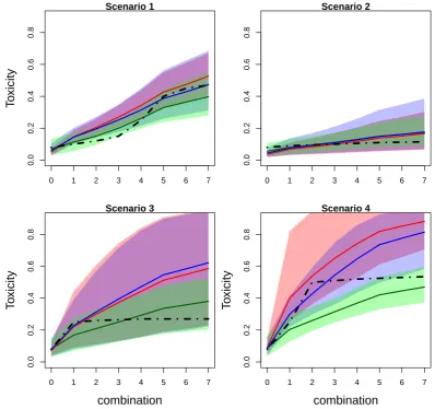
Figure 2.3: Mean values (solid lines) and 90% credible intervals (shadowed area) of toxicity probabilities for each combination obtained by fitted EmaxR (green), L2R (blue) and L2 (red) models in scenarios 1-4. True toxicity curves are marked by dashed-dotted lines. Results are based on 104 _{replications.}

(49)

in Figure 2.3 and Figure 2.4 presenting mean values of toxicity probabilities and corresponding 90% credible interval. The mean values for estimated probabilities by EmaxR (green), L2R (blue) and L2 (red) are given by solid lines while the credible intervals are given by shadow areas of the corresponding colour. The true toxicity probabilities are marked by dashed-dotted lines.

EmaxR corresponds to the best fit of the toxicity curve and to the narrowest credible interval among all alternatives in all scenarios. The fitted curves of L2R and L2 are similar for the first combinations, but probability estimates obtained by L2R are more accurate due to the shift toward the true toxicity probability curve for the rest of combinations.

2.2.6 Sensitivity Analysis

Prior Distributions In this section the influence of different sets of prior dis-tributions is studied. Since an investigator usually has a reasonable prior for E0

and the detection of a plateau should be determined by the data alone (hence an uninformative prior on theEmaxparameter is imposed), we consider cases of less informative prior forED50 and more informative one for λ

ED50 ∼Γ(0.25,0.25), λ∼Γ(3,3) (2.2.4)

and more informative prior for ED50 and less informative for λ

ED50∼Γ(1,1), λ∼Γ(0.05,0.05). (2.2.5)

We compare previously used prior distributions given in Equation (2.2.3) to the prior distributions given in Equation (2.2.4) denoted by EmaxR (λ) and the set given in Equation (2.2.5) denoted by EmaxR (ED50). The summary of the

(50)

0 1 2 3 4 5 6 7

0.0

0.2

0.4

0.6

0.8

Scenario 5

T

o

xicity

0 1 2 3 4 5 6 7

0.0

0.2

0.4

0.6

0.8

Scenario 6

0 1 2 3 4 5 6 7

0.0

0.2

0.4

0.6

0.8

Scenario 7

T

o

xicity

0 1 2 3 4 5 6 7

0.0

0.2

0.4

0.6

0.8

Scenario 8

combination

0 1 2 3 4 5 6 7

0.0

0.2

0.4

0.6

0.8

Scenario 9

combination

T

o

[image:50.595.116.512.67.633.2]

xicity

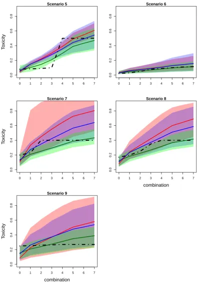
Figure 2.4: Mean values (solid lines) and 90% credible intervals (shadowed area) of toxicity probabilities for each combination obtained by fitted EmaxR (green), L2R (blue) and L2 (red) models in scenarios 5-9. True toxicity curves are marked by dashed-dotted lines. Results are based on 104 _{replications.}

(51)

[image:51.595.126.511.135.369.2]

Table 2.4: Operating characteristics of EmaxR using different prior distributions. Scenarios with no ET are underlined and the most noticeable differences across scenarios are in bold. Results are based on 104 replications.

Sc 1 Sc 2 Sc 3 Sc 4 Sc 5 Sc 6 Sc 7 Sc 8 Sc 9

Proportion of correct selections

EmaxR 45.1 94.4 44.3 82.1 57.1 97.2 64.3 29.5 21.6

EmaxR (λ) 43.8 93.3 41.3 85.5 58.7 99.7 64.1 27.3 22.7

EmaxR (ED50) 35.3 96.5 52.9 85.5 54.0 99.8 63.4 16.5 24.8

Proportion of toxicity outcomes

EmaxR 19.1 10.2 21.2 24.4 18.8 8.3 25.8 23.6 25.5

EmaxR (λ) 19.2 10.3 21.1 24.7 19.1 8.2 25.9 23.5 25.7

EmaxR (ED50) 19.1 10.5 21.1 24.5 19.3 8.4 25.4 23.5 26.1

ˆ

P

EmaxR 74.7 16.3 66.7 71.5 67.9 24.2 12.2 29.3 6.6

EmaxR (λ) 74.0 12.7 71.1 78.4 80.0 28.5 15.6 31.2 10.0

EmaxR (ED50) 68.1 9.2 66.3 70.5 61.5 23.6 16.2 20.4 11.2

NMSE

EmaxR 1.7 2.0 2.2 3.5 3.1 1.4 2.5 1.7 3.7

EmaxR (λ) 1.9 1.8 2.2 3.3 3.7 1.4 2.5 1.7 3.6

EmaxR (ED50) 2.0 2.2 2.2 4.3 3.2 1.9 3.0 2.3 3.1

lies in the middle of the curve (scenarios 1 and 8), the informative prior for ED50

results in nearly 10% loss in the PCS. Conversely, in scenario 3 where the MTC is located at the beginning of the curve, the PCS was greater. At the same time, the proportion of toxicity outcomes are not influenced by the prior choices in all scenarios.

The proportion of times the ET is found is again not affected by the choice of prior in scenarios 1-4, 6-7 and 9 with the difference between competing models below 10%. Major differences in ˆP can be found in scenario 5 in which the informative prior forλleads to 20% more false conclusions than the informative prior forED50.

At the same time, it is generally harder for EmaxR (ED50) to detect the ET with

the largest difference of 10% in scenario 8. While NMSE is not largely affected by the choice of prior distributions, EmaxR (ED50) results in slightly greater values

in scenarios 1-2, 4 and 6-8 with the greatest difference of 1 in scenario 4.