Conditional inference for possibly unidentified structural equations

Department of Economics University of Southampton Southampton SO17 1BJ UK

Discussion Papers in

Economics and Econometrics

1999

This paper is available on our website

Conditional Inference for Possibly Unidenti…ed

Structural Equations

Giovanni Forchini and Grant Hillier

University of York and University of Southampton

May, 1999

Abstract

The possibility that a structural equation may not be identi…ed casts doubt on the measures of estimator precision that are normally used. We argue that the observed identi…ability test statistic is directly relevant to the precision with which the structural parameters can be estimated, and hence argue that inference in such models should be conditioned on the observed value of that statistic (or statistics).

1 Introduction

A niggling concern for econometricians for many years has been the possibility that structural models may not be identi…ed (Sims (1980)), or may be only par-tially identi…ed (Phillips (1989)), or may involve “weak instruments” (Staiger and Stock (1997)). Recent literature on both exact distribution theory and asymptotics for this model suggests that this concern is fully justi…ed.

The work of Phillips (1983), (1989) and Hillier (1985), (1990) has made it clear that if the exclusion restrictions imposed on (the exogenous variables in) the structural equation are spurious (i.e., the structural equation is totally uniden-ti…ed), then the densities of the ordinary least squares (OLS), two-stage least squares (TSLS), and limited information maximum likelihood (LIML) estimators of the coe¢cients of the endogenous variables depend only on the error covariance matrix, and not on the structural parameters, so that none of these statistics con-tains information about those parameters. Since also standard asymptotic theory breaks down when the model is unidenti…ed, identi…cation must be presumed if these statistics are to be interpreted as usefulestimators.

Motivated by such concerns, recent literature on the distributions of the TSLS and LIML estimators has started to focus on intermediate situations where the equation of interest is neither formally identi…ed, nor totally unidenti…ed. To bridge the gap, Phillips (1989) has introduced the idea of partially identi…ed

models. These are models for which some, but not all, of the parameters are identi…ed after a rotation of coordinates in the space of both the endogenous and exogenous variables. Choi and Phillips (1992) have found that in such models the distributions of the usual estimators of both the identi…ed and the unidenti…ed coe¢cients of the endogenous variables are mean- and covariance matrix- mixed-normal. Although the density of the estimator of the unidenti…ed parameters does not depend on those parameters, it does depend on the identi…ed parameters. As far as asymptotics are concerned, the estimator of the identi…ed parameters is consistent, but conventional asymptotics does not apply. Moreover, the estimator of the unidenti…ed parameters converges in law to a non-degenerate distribution, but this is di¤erent from the small-sample distribution.

between the instruments and the included endogenous variables is assumed to be in a O(T¡1=2_{) neighbourhood of zero, where T is the sample size. Staiger} and Stock (1997) show that standard asymptotics fails for such models, and that the asymptotic distributions of the usual estimators have the same stucture as their exact distributions under normality (i.e., mixed-normal). These results lead Staiger and Stock to stress the importance of reporting the test statistic for identi…cation, but they donot indicate how the value of that statistic should modify inference, if at all.

A related recent development is based on the observation that inference on structural parameters is essentially a generalisation of the Fieller-Creasy problem (see Wallace (1980)). Sche¤é (1970) de…nes a con…dence set to beimproper if it has positive probability of being the entire parameter space. In the Fieller-Creasy problem, this probability corresponds to the probability that what is essentially anidenti…ability test statistic is small. Generalising Koschat (1987) and Gleser and Hwang (1987), Dufour (1997) has shown that in a potentially unidenti…ed structural model valid con…dence sets must be improper in Sche¤é’s sense, and argues in favour of Anderson-Rubin-type con…dence sets (a generalisation of the Fieller-Creasy solution). It is important to note that, in all three of these papers, “potentially unidenti…ed” really means that, although the model may be formally identi…ed, it is impossible to rule out a priori models that are arbitrarily close to being unidenti…ed.

In this paper we argue that the correct way to take account of the possibility that such a model may be formally unidenti…ed, or arbitrarily close to being so, is to explicitly take account of the sample evidence on the identi…cation of the model by conditioning on an identi…ability test statistic (or statistics). In particular, we argue that the reported precision of the parameter estimates should be that in the conditional distribution of the estimator given the observed value of an identi…ability test statistic, and not the unconditional precision. The analysis is exact rather than asymptotic, and supplements the work of Staiger and Stock (1997) by suggesting exactly how the identi…ability test statistic should a¤ect inference procedures for these models.

(in Section 3) apply it to the more complex problem of structural estimation. The main argument is presented in Section 2. In Section 3 we introduce the structural model, and generalise the key parts of the argument from Section 2 to this more complicated case. In Section 4 we present explicit conditional results for the OLS and TSLS estimators of the coe¢cients of the endogenous variables, and give new measures of the precision of these estimators that properly re‡ect the possibility that the model may not be identi…ed. Among our conclusions in this section is the fact that the conditional density of the OLS estimator is quite insensitive to the identi…ability statistic, while that of the TSLS estimator is sensitive to it. Thus, OLS can dominate TSLS, or vice versa,depending on the data actually obtained. Clearly, this conclusion, and its implications for applied work, are quite at odds with received opinion on inference procedures for the structural model.

2 The Argument for Conditioning

2.1 Conditioning: Post-Data Precision

Reporting the results of an inference procedure, whether it be inference about the values of unknown parameters, or a decision about whether certain propo-sitions of interest about the model under study are correct or false, entails two inter-related components: reporting the results of the procedure as applied to the data at hand, and reporting some measure of the likely precision that can be attributed to those results. For parametric estimation problems - our con-cern here - precision is usually indicated by reporting a con…dence set for the parameter(s) of interest, together with its con…dence level, or by reporting the (typically, estimated) variance or mean squared error (or approximations thereto) of the estimator chosen.

a recent discussion). The suggestion implicit here is that certain features of the sample actually obtained may be pertinent to the assessment of the precision of theestimate, but of course are immaterial to the pre-data (average) properties of theestimator.

Any attempt to assess the likely precision of an estimate - that is, to assess the likely precision of the procedure in the sample actually available - clearly (except to a committed Bayesian) must involve some sort of averaging process, but, equally, must hold certain aspects of the sample actually used …xed. In other words, whatever precision measure is used, it must, if it is to measure a property of the estimate (rather than the estimator) be conditional on certain aspects of the sample remaining …xed at their observed values. Thus, we take it as self-evident that any post-data measure of the precision of an estimate must be conditional. The problem, both in practice and from a philosophical point of view, is precisely what to condition on. That is, how can one identify events that are pertinent to the precision achieved by an inference procedure?

The only situations in which there seems to be widespread agreement among (frequentist) statisticians - both that conditioning is sensible, and upon what to condition - are those in which there is an exact ancillary statistic (cf. Cox (1958), Efron and Hinkley (1978), Barndor¤-Nielsen (1980)). This agreement is almost certainly attributable to the fact that, under suitable assumptions, it is straight-forward to show that the Fisher information based on the conditional distribution of (say) the maximum likelihood estimator given the ancillary is identical to that of the full su¢cient statistic, while the marginal density of the estimator must yield smaller Fisher information. That is, conditioning on the ancillary recovers information that would otherwise be lost. Even here the problem is di¢cult (see the collected papers by D. Basu edited by Ghosh (1988)), and outside this fairly narrow class of problems study of the problem has barely begun. It is important to notice, though, that the converse of this advice is not implied, or even sug-gested, by its adherents. The motivation for conditioning at all, whether on an ancillary statistic or not, is undeniably a concern - similar to that expressed by Lindsay and Li - to obtain a more relevant measure of the inferential precision actually achieved in the sample (see also Barndor¤-Nielsen’s comments on the paper by Efron and Hinkley (1978), and the discussion in Chapter 2 of Cox and Hinkley (1974)).

we shall advocate, for a particular class of problems to be described shortly,

conditional measures of precision, and for precisely the reason that applies in the wider problem: to obtain a more relevant measure of the precision achieved

in the sample actually available. As noted above, the problem is to identify aspects of the data that are pertinent to the precision of the estimate, and we shall argue that, in the types of models we are considering, the structure of the problem clearly identi…es which events a¤ect precision. We begin by discussing the simplest possible example of the type of problem we shall be concerned with - the Fieller-Creasy problem.

2.2 The Fieller-Creasy Problem

The Fieller-Creasy problem is a celebrated, apparently straightforward, inference problem that produces “paradoxical” assessments of precision, namely improper con…dence sets (see Wallace (1980) for an historical survey of the problem). The problem contains virtually all the essential features of the structural model that is our main concern, and is also closely related to the linear calibration (inverse re-gression) problem (Hoadley (1970), Dobrigal, Fraser, and Gebotys (1987), Gleser and Hwang (1987)), errors-variables regression, some principal component in-ference problems, and inin-ference on ratios of regression parameters.

Assume that the 2£1 vectors xi(i = 1,....,n) are independent N(¹, ¾2I2), and that we are interested in either the ratio of means à = ¹₁=¹₂; or in the direction of the vector¹, parameterised by the angle, Á, when ¹ is expressed in polar coordinates in the usual way. The vector of sample means, x¹, and

s2=

n

X

i=1

£

(x1i¡x¹1)2+ (x2i¡x¹2)2

¤

;

are jointly su¢cient for (¹; ¾2_{),x¹»N(¹;(¾}2_=n)I

2); x¹ is independent of s2; and s2_=¾2 _{» Â}2_{(2 (n¡1)). The maximum likelihood estimator for à is Ã^ = ¹x}

1=x¹2, but the (unconditional) variance of _Ã^ _{does not exist. Fieller (1954), and Creasy}

(1954) considered the problem of constructing a con…dence interval for Ã, and

the standard “Fieller solution” is based on the observation that

n(¹x1 ¡Ãx¹2)2=¾~2

¡

1 +Ã2¢_»F (1;2 (n_¡1)); (1)

(a) the entire real line if kx¹k2 = (¹x2

1+ ¹x22) < c = ~¾2F®(1;2 (n¡1))=n, where

F®(º1; º2) is such that PrfF (º1; º2)< F®(º1; º2)g= 1¡®; (b) the interior of a …nite interval ifx¹2

2 > c, and (c) the exterior of a …nite interval if kx¹k2 > c and x¹2

2 < c.

Thus, it is entirely possible for, say, the 90% con…dence interval for à to consist of the whole real line, and the (unconditional) expected length of the interval is in…nite.

She¤é (1970), James, Wilkinson, and Venables (1974), Dobrigal, Fraser, and Gebotys (1987), and Koschat (1987) all treat the problem in terms of the interest parameterÁ, rather thanÃ. Essentially the same paradox arises although, as we

shall see, there is a subtle di¤erence between the two versions of the problem. Koschat (1987), for this problem, and Gleser and Hwang (1987) for a wider class of closely related problems, have shown that problems of this type have the property that every con…dence set with non-zero con…dence coe¢cient must have positive probability of being the entire parameter space, and hence must be improper in Sche¤é’s (1970) sense. Hence, the di¢culty is not peculiar to the Fieller solution. Dufour (1997) has extended these results to the structural model, and other models of interest in econometrics.

2.3 Interest Parameters and Critical Sets

Now, notice that in the above Fieller problem, there is certainly no di¢culty in obtaining an always-bounded con…dence set for the underlying parameter vector

¹. The region (sphere) de…ned by the acceptance region for a likelihood ratio

test:

F =n(¹x_¡¹)0_{(¹x¡¹)=2~¾}2 _{< F}

®(2;2 (n¡1)) (2)

is the most obvious candidate. Apart from being the likelihood ratio statistic,

F is the (unique) maximal invariant (under the group of transformations G =

f(a; H); a >0; H(2_£2) orthogonalgacting on the statistics (¹x_¡¹; s2_{) by:}

((¹x¡¹); s2)¡!(aH(¹x¡¹); a2s2):

Thus, con…dence regions for¹based onF characterise the entire class of invariant

regions.

observation, it seems clear that the “Fieller paradox” derives from the properties of the mapping [underlying parameters] _¡! [interest parameter], and not from any intrinsic property of the embedding model. We shall see shortly that this observation also applies to the structural model, but before doing so we elaborate on its implications for the Fieller problem itself, where the situation is simpler.

If ° =°(¹) is an everywhere continuous one-to-one function of ¹, the image of any closed bounded set of¹-values is a closed bounded set of °-values, so that

the (proper) con…dence set (2) for¹naturally induces a proper con…dence set for ° (with the same con…dence level). In this sense, inferential results for¹are suf-…cient for inference about any everywhere continuous and 1-1 function of¹; and

it seems reasonable to assert that, in these circumstances, there is no essential di¤erence between the inference problem for ¹ and that for (any such function)

°. Of course, actual measures of precision, like estimator variances, or Fisher

information, change under reparameterisation, but, although seldom stated ex-plicitly, estimator loss functions would usually embody exactly this invariance under smooth reparameterisations, and so re‡ect the main idea.

On the other hand, the key characteristic of (both versions of) the Fieller problem is that the mapping from the underlying parameter ¹ to the interest parameter à (or Á) is not everywhere continuous and one-to-one. In the case of

the interest parameterÃ, the mapping¹_¡!(Ã; ¹₂)(fromR2 _toR2_{) is continuous} and 1-1 everywhere except along the ¹₁ axis, where à can take any value. In the case of the interest parameter Á, the mapping ¹ _¡! (Á; ½) (where ½ = _k¹_k) is continuous and 1-1 everywhereexceptat the origin (¹= 0), whereÁcan take any value. Dufour (1997) calls such subsets of the parameter spacenon-identi…cation subsets, but we shall refer to them as critical sets. Notice that the critical set depends on the de…nition of the interest parameter(s) in terms of the parameters of the embedding model.

The Fieller solution (1) is easily obtained from (2). The line ¹₁ ¡Ã¹₂ = 0

intersects the spherekx¹¡¹k2 < f just if (x¹1¡Ãx¹2)2=(1 +Ã2)< f: The induced (Fieller) con…dence set for à is thus the set for which this line intersects the sphere, and is a …nite interval if the sphere does not cross the ¹₁-axis ( i.e.,

¹

x2

2 > f), is the exterior of a …nite interval if the sphere crosses the ¹1 axis but does not include the origin, (i.e., x¹2

2 < f but kx¹k 2

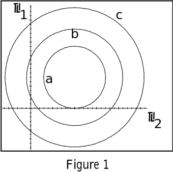
> f), and is the entire real line if the sphere contains the origin (i.e. kx¹k2 < f) - see Figure 1 below, where

that, for either version of the Fieller problem, the region (2) must intersect the critical set for some values of (x; s¹ 2_{), unless it has con…dence level zero. That is,} every con…dence set forà (or Á) induced by (2) must be improper unless it has con…dence level zero.

a b

c

µ µ₁

2

Figure 1

We now generalise these observations on the Fieller problem to an arbitrary model in which the interest parameter can take any value on a subset of the full parameter space for the embedding model.

An Index of Precision

Generalising the Fieller problem, letp(x;µ)denote the model density for either

the sample data or the minimal su¢cient statistic, withµ ₂M _½Rk_{, and consider}

a reparameterisation° :M _¡!¡ _½Rk_{: We assume that the interest parameter}

°1 is a subvector of °, and, as above, that there is a non-empty subset C ½ M such that, forµ ₂C, °₁ can take any value in some set ¡1 of dimension greater than one. That is, for µ ₂ C; the mapping ° becomes a correspondence, not a function. We callC thecritical subset ofM (for the interest parameter°₁). Note

that membership of C is an attribute ofµ; not of °₁. Let ^µ denote the MLE for µ;and let

LRc(x) =

n

µ;p(x;µ)=p(x; ^µ)> co;0< c < 1; (3) denote the con…dence region forµbased on the acceptance region for a likelihood ratio test. The con…dence level is determined by the choice of c, with smaller

values ofccorresponding to larger con…dence levels.

numerator by its maximum value over parametersnotinvolved in the de…nition of °₁, and the denominator by its maximum over the values of all parameters. For expository purposes we work with the simplest case. We assume that the regions (3) are bounded with probability one. Obviously, the acceptance region based on any testing principle could be used in place of (3), with obvious modi…cations to the argument that follows.

For …xed data x, and a …xed critical set C, there are two possible outcomes

for the region (3):

(a)LRc(x)intersectsC for all, or all but very large, values ofc. That is,LRc(x)

is “close to”Cfor all but very large values ofc. In this case the induced con…dence

region for°₁ will be the entire set¡1 for all but very small con…dence levels, and it seems reasonable to conclude that,with this particular data x,°₁ is determined with “low precision”;

(b)LRc(x)andCmay be disjoint for all but very small values ofc(of course, they

cannot be disjoint for allcif Cis non-empty). That is,LRc(x)is “remote from”

C for all but very large con…dence levels. In this case it seems reasonable to

conclude that,with this particular data x, °₁ is determined with “high precision”. If we take as given the standard (frequentist) position that con…dence sets are an adequate, if somewhat philosophically problematic, representation of the precision of an inference, these remarks suggest that the location of LRc(x) in

relation to the critical set C has, for problems of this type, a direct bearing on the precision with which°₁ can be learnt from the data available. Moreover, they immediately suggest an intuitively reasonable “post-data index of precision” for inference about°₁ in the type of problem we are considering, namely:

k(°1;x) = 1¡c0;0< k <1; (4)

with c0 the smallest value of c in (3) for which LRc(x) does not intersect C.

For, if c0 is near 1 only very “small” regions (i.e., low con…dence levels) for µ would be compatible with a non-trivial region for °₁ (with the given data), and

Remarks

1. IfC is empty, so that the mappingµ _¡!° is everywhere 1-1, c0 = 0, because LRc(x) can be made as large as we like without intersecting C. Thus, in this

case, k= 1 for any x, and the precision with which any everywhere 1-1 function ofµ can be located is identical to that with whichµ itself can be located, as seems

natural.

2. If, with the data available, LRc(x) intersects C for all c, c0 = 1;and k = 0, indicating that, with this data, there is no prospect of locating °₁.

3. Although the acceptance region for any test on µ could be used as the un-derlying con…dence set for µ, that based on the likelihood ratio in (3) has the

advantage that di¤erent choices for the mappingµ ¡!° that leave the interest

parameter°₁ invariant will leave k invariant.

4. k is evidently a monotonic increasing function of the maximum con…dence level (for likelihood ratio based con…dence sets for µ) that (with the given data)

is compatible with a non-trivial con…dence set for the interest parameter°₁. This maximum compatible level (mcl) could itself be used as an index of precision (see Table 1 below).

5. The precision for inference about the interest parameter,°₁, has been de…ned so as to depend on the entire vectorµ, because membership of the critical setCis an attribute ofµ,not °₁. In this respectk re‡ects information in the data about

both “nuisance parameters” and the “interest parameter”. This, it seems to us, is natural when the true source of the inference problem has been recognised. 6. Since, under regularity conditions, the power of the likelihood ratio test goes to unity asn_{! 1}, it is clear from (5) that, providedµ =₂C,k _!1in probability as n _{! 1}. That is, the precision with which °₁ can be located will, if µ =₂ C, approach 1 as the sample size increases. Just as importantly, the converse is also easily seen to be true: if µ ₂ C, the precision, k, goes to zero in probability as

n_{! 1}.

In both versions of the Fieller problem above, the second component of the transformation¹_! ° (in the …rst case, ¹₂, in the second, ½ ) is constant (zero) on the critical setC. In the general case, the transformationµ _!° = (°₁; °₂)can usually be chosen so that°₂ vanishes onC. The implication of this remark, then,

or on the sample evidence on the value of °₂. In fact as we shall see shortly

-this evidence is encapsulated in the precision index, k.

Now, as initially de…ned, k measures how remote (or otherwise) likelihood ratio based con…dence regions forµ are from the critical set C. It is easy to see,

however, that k is completely determined by the likelihood ratio test statistic for testing the hypothesis H0 : µ 2 C against an unrestricted alternative. For, denoting this test statistic byLR(C), we have,

k = 1_¡sup

µ2C

"

p(x;µ)

p(x; ^µ) #

= 1_¡LR(C): (5)

Hence, the post-data precision for°₁, as measured byk(°₁;x), will be large just if the likelihood ratio test statistic for testingµ2C is small (suggesting rejection),

and vice versa.

Examples: For the two versions of the Fieller-Creasy problem we have:

1. Interest parameter Ã: In this case the critical set C = f¹:¹₂ = 0g, and the region F < F® in (2) cuts the ¹1-axis unless F® f2=2 = nx¹22=2~¾2. Hence, for inference about the ratio of means,Ã:

k¡Ã; ¹x; s2¢ = 1¡

µ

1 + f2

2 (n¡1) ¶¡n

:

2. Interest parameter Á: The largest value ofF® such that the regionF < F® in

(2) does not intersect C =f0g is clearly f1 = nkx¹k2=2~¾2. Hence, for inference about the direction of¹:

k¡Á; ¹x; s2¢ = 1¡

µ

1 + f1

n¡1 ¶¡n

:

Note that, as one would expect, k depends on the sample size, n. Clearly, k

di¤ers in these two versions of the Fieller problem precisely because the interest parameter, and hence the critical setC, di¤ers.

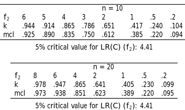
Some values of the precision index k for the Fieller problem with interest parameterà are given in Table 1 below. As an example, if the observed value of f2is 1, andn= 20, the maximum con…dence level (mcl) for which the con…dence region (2) just intersects the ¹1-axis is .389, and the corresponding index of precision forÃ, k, is .405. Both numbers indicate that à is poorly determined

Table 1: Values ofk and maximum con…dence levels

n= 10

f2 6 5 4 3 2 1 .5 .2

k .944 .914 .865 .786 .651 .417 .240 .104

mcl .925 .890 .835 .750 .612 .385 .220 .094 5% critical value for LR(C) (f2): 4.41

n= 20

f2 8 6 4 2 1 .5 .2

k .978 .947 .865 .641 .405 .230 .099

mcl .973 .938 .851 .623 .389 .220 .095 5% critical value for LR(C) (f2): 4.41

The argument above establishes that, for any problem of the type we are interested in, LR(C) is clearly relevant to the precision with which, with the

given data, the interest parameter °₁ can be located, from a frequentist point of view. Various other treatments of the problem can also be invoked to the same end. First, for the Fieller-Creasy problem (and hence the inverse linear regression/calibration problems), Hoadley (1970) has shown thatLR(C)emerges naturally as an index of precision when the problem is viewed from a Bayesian perspective. In particular, under Hoadley’s assumptions, the posterior density is more sharply peaked the larger isLR(C). Second, using a …ducial argument, Dobrigal, Fraser, and Gebotys (1987) suggest con…dence sets (for the angle, Á,

in the polar coordinate version of the Fieller problem) conditioned on the value of LR(C). The length of the interval suggested decreases with LR(C), but the interval is always bounded. Finally, it is not di¢cult to show that, for the Fieller problem in either form, the shape of the likelihood function near its maximum depends heavily on LR(C), so that adherents to the strict likelihood principle (including Edwards (1970)) would use LR(C) to indicate how accurately the MLE is determined. Thus, whatever one’s statistical persuasions, for problems of this type the observed value of the likelihood ratio test statistic for testing

To summarise, we have argued that:

(a) Inference problems, like the Fieller problem, and the structural equation model, can usually be embedded in a model for which no paradox arises;

(b) The problem arises because the reparameterisation involved in the de…nition of the interest parameter entails acritical set in the embedding parameter space on which the interest parameter can take any value in a set of dimension greater than one;

(c) The likelihood ratio test statistic for testing whether, in the embedding model, and with the data actually available, the parameter lies in the critical set, is a natural measure of the ability of the sample to inform about the interest param-eter;

(d) Far from being a “nuisance”, the sample evidence on the non-interest param-eter component of the reparamparam-eterised model is directly relevant to the precision with which the interest parameter itself can be located.

Our conclusion is that the observed likelihood ratio test statistic for testing membership of the critical set is directly relevant to the precision with which the interest parameter can be estimated, and that it therefore makes no sense to average over values of that statistic that have not occurred. That is, we conclude that any sensible assessment of the properties of estimates of the interest parameter(s) must be made conditional on such a test statistic (or other relevant indicators of critical set membership).

Before applying this argument to the structural equation model, we end this section with some further remarks on the “Fieller solution” that are also pertinent in the structural equation context.

2.4

Further Remarks on Fieller’s solution

In seeking a basis for making con…dence statements about an interest parameter, say °₁, it is common practice to seek a pivotal function, Q(x;°₁) say, that is a function of the data and the interest parameter, but not a function of nuisance parameters. That is, a function whose (unconditional) distribution (induced by the density of x, p(x;µ)) does not depend on unknown parameters (cf. Basu

(1981), reprinted in Ghosh (1988)). If ¡1 is the parameter space for °1, and X the sample space for x, the inequality Q(x;°₁) < q (say) de…nes a subset Eq,

value of x is the x-section of Eq, Eqx = f°1 : (x; °1)2Eqg. The con…dence level

´(q) corresponding to q is ´(q) = Pr_fQ(x;°₁)< q_jµ_g, which, if Q is pivotal, does not depend on µ. The set Ex

q is the con…dence set estimator for °1, and the pair ¡Ex

q; ´(q)

¢

together are usually interpreted as indicating the precision with which °₁ is determined by the data. The motivation for using a pivot in the construction of¡Ex

q; ´(q)

¢

is, of course, that´(q)can, in principle, be known exactly.

As Example 6 in Basu (1981) makes clear, the interpretation of Ex q as a

con…dence set estimator for °₁ (and hence an indicator of the precision with which°1 is determined by the data) depends on the knowledge that x contains information on °₁, but certainly does not imply that it does. In other words, a minimal necessary condition for the setEx

q (induced by the pivotal quantity Q)

to reveal anything about°₁ is that it isknown that the observed xcontains (in

some other sense) information about °₁. At the very least, the density p(x;µ)

must vary with°₁ under the reparameterisationµ _!°.

Now, in the cases we are concerned with here, it is known that, in the under-lying parameterisation of the modelp(x;µ), there is a critical set C for which°₁

can take any value. Hence it is known that (whatever de…nition of “information” is adopted) the datamay be uninformative about°₁, but it is not known whether µ ₂ C or not. We now consider the implication of this for the Fieller solution

itself.

The interpretation of the Fieller-Creasy problem above throws the Fieller solution into doubt, because, as we shall now show, the statistic upon which it is based is either pivotal and uninformative about the interest parameter, ornot

pivotal with respect to the family of underlying modelsp(x;µ), and´(q)can be

arbitrarily small. We discuss only the case of the interest parameter Ã; similar

remarks apply in the case of the interest parameter Á. The quantity Q(¹x; s2_{;Ã) = n(¹x}

1¡Ãx¹2)2=¾~2

¡

1 +Ã2¢ on which the Fieller

solution is based is pivotal for the interest parameter Ã, provided ¹ =2 C, in

the sense that, for ¹ =₂ C satisfying ¹_{1 ¡}ù₂ = 0 (but not otherwise), Q _» F (1;2 (n¡1)). What can be said about the distribution Q when µ 2 C? It

seems to us that there are two possibilities:

(1) If it were true that ¹₂ = 0 implied ¹₁ = 0, as is the case under the reparameterisation ¹ = (ù₂; ¹₂)0 used above, then it would remain true that

could claim toknow that, for every member of the family of densities p(x;¹; ¾2_), ¹₂ = 0 implies ¹₁ = 0; and this in fact is the maintained hypothesis in both the calibration problem and the structural equation model. Note, however, that this interpretation of the problem is clearlynot implied by merely declaring the interest parameter to beà =¹₁=¹₂.

Taking this point of view, though, implies that, when ¹₂ C, (a) p(x;¹; ¾2_), when reparameterised in terms of (Ã; ¹₂; ¾2_{), does not depend on Ã; (b) Q is} ancillary for all real Ã; (c)Ã is arbitrary in this parameterisation. These are all

simply di¤erent manifestations of the same phenomenon: that the transformation

¹!(Ã; ¹2)is not one-to-one when¹2 = 0. Clearly, since it isnot known whether ¹ ₂ C or not, the “con…dence set” induced by Q has nothing whatever to say about either the value of Ã, or the precision with which it has been located by the data.

(2) If, instead, one takes the view that, when ¹ ₂ C, ¹₁ is arbitrary, then, for ¹₂C,Qhas the non-centralF0_{(1;2 (n¡1); ¸)distribution, with non-centrality}

parameter ¸ =n¹2 1=

¡

¾2¡_{1 +Ã}2¢¢_{, for every real Ã. Hence, under this} interpre-tation,Q, isnot pivotal with respect to the entire family of distributionsp(x;µ): its distribution depends on whether µ ₂ C or not. In fact, when ¹ ₂ C, the “con…dence level” ´(q) = PrfQ < qg can be arbitrarily small, because the non-centrality parameter ¸ can be arbitrarily large. It seems clear that, under this

interpretation of the problem, it would be quite unreasonable to claim that the “con…dence set” induced by Q, and its “con…dence level” (calculated assuming

¹₁ = 0), have, by themselves, anything to (unambiguously) say about the interest parameterÃ.

Thus, both interpretations of the Fieller problem leave the “Fieller solution” in doubt. Exactly analogous di¢culties arise in the interpretation of Anderson-Rubin con…dence regions for the coe¢cients of the right-hand-side endogenous variables in the structural equation model - the “solution” favoured by Dufour (1997). The point, of course, is that the sample does contain information on whether or not ¹ ₂ C, and this information is ignored when the inference is based onQ(¹x; s2_{;¹)(and its “con…dence level”) alone (although itis re‡ected in} the “con…dence set” that this produces).

Sche¤é’s (1970) advice is to report the Fieller interval if it is bounded, and to declare that nothing has been learnt aboutà if not - a kind of informal

level achieved by this procedure is strictly less than the nominal level implied in (1). A second possibility would simply be to report the value of the maxi-mum likelihood estimator,_Ã^_{, together with our suggested measure of precision,}

k, or, equivalently, the likelihood ratio test statistic for testing H0 :µ 2C. This is essentially the advice o¤ered by Staiger and Stock (1997) for the structural equation model, although without the interpretation we have given here. For precision measures based on con…dence sets, therefore, the suggestion would be to report the value of k, or, equivalently, the largest con…dence level for which

the con…dence region forµ in the underlying model just intersects the critical set

C.

For point estimation problems our suggestion is to report the conditional variance of the estimator of interest, or, more completely, its conditional density, conditional on the observed value(s) of the relevant identi…ability test statistic(s). We turn now to an investigation of the implications that this advice has for inference in the single strucural equation model.

3 The structural equation model

We consider a single structural equation written without explicit normalization:

Y ¯_M =Z1°+u; (6)

where Y is a T £(n+ 1) matrix of endogenous variables, Z1 is a T £k1 matrix of exogenous variables, and ¯_M and ° are, respectively, (n+ 1)_£1 and k1£ 1 vectors of parameters. The reduced form corresponding to (6) is

Y =Z1© +Z2¦ +V; (7) whereZ2 is aT £k2 matrix of exogenous variables not included in the structural equation, © and ¦ are matrices of parameters of dimension k1 £(n+ 1), k2 £

(n+ 1) respectively. We assume throughout that k2 ¸ n. The rows of V are assumed to be independent normal vectors with mean zero and common

(n+ 1_£n+ 1) covariance matrix

- = µ

!11 !021 !21 -22

¶

;

parameters.

Compatibility of the structural equation (6) and reduced form (7) requires the existence of some¯_M6= 0, such that

¦¯_M = 0; (8)

©¯_M = °, V ¯_M = u. Note that (8) implies rank (¦) n. If rank (¦) = n, equation (8) uniquely determines the direction of ¯_M (i.e., ¯₄ is restricted to

lie in a one-dimensional space): If rank (¦) < n, ¯_M can be written as a linear

combination of then_¡rank (¦) basis vectors spanning the space orthogonal to the space spanned by the rows of ¦. Thus, in this case ¯_M lies in a space of dimension greater than one. Our assumptions about rank (¦) will be discussed shortly.

The structural equation is usually normalized by setting ¯_M = (1;¡¯0₀)0, and ¦ = (¼1;¦2), so that (8) becomes

¼1¡¦2¯0 = 0; (9)

and the structural equation (6) has the form

y1 =Y2¯0+Z1°+u: (10) Note that this normalisation impliesrank(¦)< n+ 1; and ¯₀ is uniquely

deter-mined if the rank of ¦2 is n. Equation (10) is identi…ed if rank (¦2) = n; and is totally unidenti…ed if¦2 = 0. In all other cases we have a partially identi…ed structural equation, where some of the parameters are identi…ed after a rotation of coordinates in the space of the endogenous variables (Phillips (1989)). It is well known (Phillips (1983), Hillier (1985)) that the densities of the OLS, the TSLS, and the LIML estimator of¯₀ (and ¯_M) are free of any of the parameters

in (10) and the estimators are therefore uninformative about them, when the structural equation is totally unidenti…ed. Moreover, in this case, the densities of the TSLS and the LIML “estimators” do not depend on the sample size, so that conventional asymptotics for these “estimators” break down.

formally identi…ed, but that points in ¦2-space arbitrarily close to the critical setC =_f¦2 : rank (¦2)< ng cannot be ruled outa priori. As shown by Gleser and Hwang (1987) and Dufour (1997), the model can be totally uninformative about the interest parameter if there exists a sequence of points in the¦2-space converging to some point in the critical set. Exactly as for the Fieller-Creasy problem discussed in the previous section, the sample evidence on the distance of ¦2 from the critical set re‡ects how well (or how poorly) ¯0 can be located

with the data actually available. And, as argued above, this suggests that the relevant post-data properties of estimates of¯₀ (including measures of precision) are thoseconditional on that evidence.

We consider the OLS and the TSLS estimators of ¯₀ in (10), which can both be written in the form:

b = (Y₂0P Y2)¡1Y20P y1

with, in the OLS case, P = PZ1, where PA = I ¡A(A0A)¡1A0 for any matrix

A, and in the case of TSLS, P = PZ1 ¡PZ, where Z = (Z1; Z2). Joint minimal su¢cient statistics for¦; ©and- in (7) are:

^

© = (Z₁0Z1)¡ 1

Z₁0Y;

^

¦ = (Z₂0PZ1Z2)¡1Z20PZ1Y;

S = Y0PZY;

and these remain minimal su¢cient for any¦withrank(¦)>0. These statistics

are independent of each other, and

^

© _» N³© + (Z₁0Z1)¡1Z10Z2¦;(Z10Z1)¡1-

-´

;

^

¦ » N³¦;(Z₂0PZ1Z2)¡1-

-´

; S _» Wn+1(À¡k2;-);

whereÀ =T ¡k1.

Partitioning_{¦ =}^ ³_¼^1;¦^₂´_{, and S comformably with-,}

S = µ

s11 s021 s21 S22

¶

;

inference about¦2 can be based on the matrix pivot

F¦2 =S

¡12

22

³ ^ ¦2¡¦2

´0

Z₂0PZ1Z2

³ ^ ¦2¡¦2

´

S¡12

which has the matrix-variateF-distribution (Muirhead (1982) Theorem 10.4.1.).

Using the acceptance region for the likelihood ratio test, a con…dence region for¦2 can be constructed by …nding all values of ¦2 for which

jIn+F¦2j< c: (12)

This is the analogue of (2) for the Fieller problem. The con…dence region for

¦2 based on (12), P = f¦2 :jIn+F¦2j< cg; intersects the critical set C =

f¦2 : rank (¦2)< ng only ifcis larger thanmin¦22CfjIn+F¦2jg. Let f1 f2

::: fn be the ordered eigenvalues of

F0 =S¡

1 2

22 ¦^02Z20PZ1Z2¦^2S¡

1 2

22 : (13)

It is straightforward to check that the region (12) intersects the critical setCjust iff1 < c, and that the post data index of precision for the interest parameter¯0 (de…ned in (4)) is, in this case:

k³¯₀; ^¦2; S22

´

= 1_¡(1 +f1)¡ T

2 : (14)

The quantity (1 +f1)¡ T

2 is the likelihood ratio statistic for testing the null

hy-pothesis that rank(¦2) n¡1 against the alternative that rank(¦2) =n. In the case n = 1 the argument in Section 2 suggests that inference on ¯₀

should be made conditional on the observed value of f1. In particular, the preci-sion (variance) reported for an estimate of ¯₀ should be that in the conditional density of the estimator given the observed value of f1. In the case n > 1 the same argument (based on the con…dence region for¦2 induced by the acceptance region for the likelihood ratio test) would also suggest conditioning on f1 alone. However, the likelihood ratio test principle is, in the case n > 1, only one of a

number of plausible candidates for constructing con…dence regions for¦2 :there is, in this case, no unique optimal invariant test. In fact, we now argue that, for the casen >1, a case can be made for conditioning on alln eigenvalues ofF0.

The problem of testingH0 : ¦2 = ¦¤2 (a particular value of¦2) can be reduced by su¢ciency and the fact that the hypothesis does not involve©;to tests based on( ~¦2; S22); where ¦~2 = (Z20PZ1Z2)

1

2¦^₂. But, for tests based on

³ ~ ¦2; S22

´

group of n£n non-singular matrices), with group operation (¡1; E1)(¡2; E2) =

(¡1¡2; E1E2), acting on the space of statistics

³ ~ ¦2; S22

´

by (¡; E)( ~¦2; S22) =

(¡ ~¦2E0; ES22E0), and with induced group of transformations on the parameter space given by (¡; E)( ¹¦2;-22) = (¡ ¹¦2E0; E-22E0), where ¦¹2 = (Z20PZ1Z2)

1 2 ¦

2. Under the group of transformations G, a maximal invariant is (f1; :::; fn), where

f1 ::: fn are the eigenvalues of F0 in (13). Moreover, the distribution of

(f1; :::; fn) depends only on the eigenvalues of ¤ = -¡ 1 2

22 ¦¹02¦¹2-¡

1 2

22 ; the maximal invariant under the induced group of transformations on the parameter space. (Muirhead (1982), Theorem 6.1.12).

Since every invariant test depends only on the maximal invariant, and the likelihood ratio test is just one member of this class, it seems preferable in the case

n > 1 to condition on the full maximal invariant rather than on any particular

scalar function of(f1; :::; fn). Thus, in the casen > 1, we shall condition on all n

roots (f1; ::::; fn)of F0. In Appendix A we derive the conditional densities of the OLS and TSLS estimators for¯₀ in (10), conditional on the full maximal invariant

(f1; :::; fn). Since the exact results for the general case of n + 1 endogenous

variables are di¢cult to interpret, in the next Section we analyse in detail the results for the case n= 1;for which the identi…cation test statistic is simply f1.

4 Conditional Results for the case n = 1

4.1 Conditional Densities and Moments

In this section we analyse the consequences of conditioning on f1 for the OLS and TSLS estimators of ¯₀ in (10), assuming n = 1. Note that, when n = 1,

f1 = ^¦02Z20PZ1Z2¦^2=S22 is a scalar, and we shall denote this simply byf. Ideally we would want to obtain the analogous results for the LIML estimator as well, but these have so far proved intractable. To simplify the notation, but without loss of generality, we employ the standardizing transformations described in Phillips (1983). For either estimator,b, for¯₀, de…ne the transformed statistic

r = (-1₂₂=2b_¡-₂₂¡1=2!21)=!; (15) and the transformed parameter:

where

!2 =!11¡!210 -¡221!21: (17) Note that, in the case n = 1, the squared correlation between Y2 and u is ½2 = ¯2=(1 +¯2).

The exact conditional densities of rOLS andrT SLS, givenf, are given in

The-orem 1. These results are derived in Appendix A, where we also derive the analogous results for the general case (n > 1). The conditional means, variances, and mean-square-errors are given in Theorem 2, and the proofs of these results are given in Appendix B.

Theorem 1 Conditional Densities: Given the model speci…ed in Section 3 with

n= 1, and the standardization described above:

The conditional densities of the OLS and TSLS estimators, given f, are:

pdfOLS(rjf) = [B(

1 2;

À

2)]

¡1_{(1 +r}2₎¡À+1 2

1

X

j=0

g1j(¸; ¯;f)

"

¸f(1 +¯r)2 (1 +f) (1 +r2₎

#j

;

(18)

and

pdfT SLS(rjf) = [B(

1 2;

À

2)]

¡1₍₁₊ fr2

1 +f)

¡À+1 2

1

X

j=0

g2j(¸; ¯;f)

"

¸f(1 +¯r)2 (1 +f)(1 + ₁₊fr2_f)

#j

;

(19)

where B(a,c) = ¡(a)¡(c)=¡(a+c); À = T _¡k1; ¸ = ¦02Z20PZ1Z2¦2=2-22 is a

scalar,

g1j(¸; ¯;f) =

¡_À+1

2

¢

j

j!¡k2

2

¢

j

1F1

³

j+1 2; j +

k2

2 ;¡

¸f ¯2

1+f

´

1F1

³ À 2; k2 2 ; ¸f 1+f

´ ; (20)

and

g2j(¸; ¯;f) =

¡_À+1

2

¢

j

j!¡k2

2

¢

j

f12₁F₁¡j+ 1

2; j+

k2

2;¡¸¯ 2¢

(1 +f)12₁F₁

³ À 2; k2 2; ¸f 1+f

´ : (21)

In the totally unidenti…ed case (¸= 0), rOLS and f are independent and

pdfOLS(rjf) =pdfOLS(r) = [B(

1 2;

À

2)]

while, for the TSLS estimator:

pdfT SLS(rjf) = [B(

1 2;

À

2)]

¡1_{(f=(1 +f))}1_{2(1 +} fr2

1 +f)

¡À+1

2 : (23)

Theorem 2 Conditional Moments: For non-negative integers p and q, let

pHq(z) =

1F1(À₂ ¡p;k2₂ +q;z) 1F1(À₂;k2₂;z)

; (24)

and

pHq¤(z) =

2F2(À₂ ¡p;3₂;1₂;k2₂ +q;z) 1F1(À₂;k2₂;z)

: (25)

In the following expressions, z =¸f=(1 +f):

(i) the conditional means are:

ET SLS(rjf) =

2¸¯ k2 0

H1(z); (26)

EOLS(rjf) =

f

(1 +f)ET SLS(rjf) = 2z¯

k2 0

H1(z); (27)

(ii) the conditional variances are:

V arOLS(rjf) = (À ¡2)¡1[1H0(z) +

2z¯2 k2 1

H₁¤(z)]_¡[2z¯

k2 0

H1(z)]2; (28)

V arT SLS(rjf) = (f(À¡2)=(1+f))¡1[1H0(z)+

2¸¯2 k2 1

H₁¤(z)]_¡[2¸¯

k2 0

H1(z)]2; (29)

(iii) the conditional mean-square-errors are:

M SEOLS(rj f) =¯2 + (À¡2)¡1[1H0(z) +

2z¯2 k2 1

H₁¤(z)]_¡ 4z¯

2 k2 0

H1(z); (30)

MSET SLS(r j f) =¯2+ (f(À¡2)=(1 +f))¡1[1H0(z) +

2¸¯2 k2 1

H₁¤(z)]

¡4¸¯ 2 k2 0

Remarks

1. When the structural equation (10) is totally unidenti…ed the OLS estimator is independent of f, but this is not the case for the TSLS estimator. In general, conditioning a¤ects the properties of both the OLS and the TSLS estimators. More precisely, conditioning makes the functional forms of the densities of the OLS and TSLS estimators di¤erent (even though their unconditional densities have the same functional form), and thus has an impact on the choice between these estimators (see below).

2. The leading terms in the densities of the OLS and TSLS estimators (i.e., equations (22) and (23) respectively) are both proportional to a Student-t den-sity withÀ degrees of freedom, so that integer (conditional) moments exist up to orderÀ_¡1, and the variances are(À_¡2)¡1 _{and(f(À¡2)=(1 +f))}¡1 _{respectively.} For the TSLS estimator unconditional integer moments exist only up to order

k2¡1.

3. As in the case of the unconditional densities (see Phillips (1983)), the condi-tional densitiespdfOLS(rjf)andpdfT SLS(rjf)are not symmetric about¯, except

when¯ = 0.

4. From equation (27) it is clear that jEOLS(rjf)j < jET SLS(rjf)j, that is, the

conditional mean of the OLS estimator is always closer to the origin than that of the TSLS estimator, by a factor that depends onf. We shall see shortly that,

as this result suggests, the OLS estimator can certainly conditionally dominate the TSLS estimator for small values of both¯ and f: Mean-squared-error com-parisons of the two estimators are given in the next subsection.

4.2 Numerical properties

The conditional densities of the OLS and TSLS estimators are characterized by the three known quantities (À=T_¡k1, k2,f), and the two unknown parameters

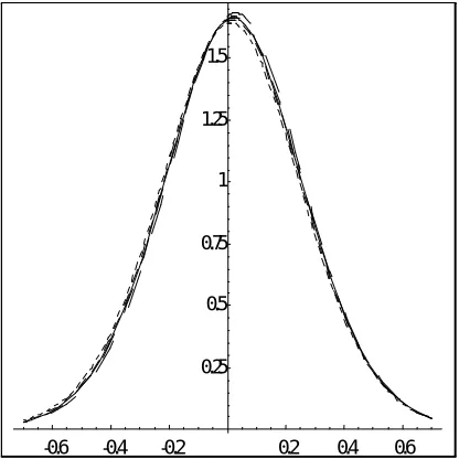
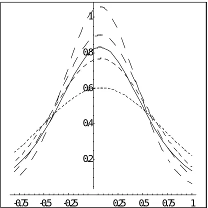
(¸, ¯):Figures 2 and 3 illustrate the e¤ects of conditioning. Plots of the densities given in Theorem 1 have been drawn for ¯ = 0:35, ¸ = :5 and T = 20, k1 =

3, k2 = 4 (this choice of values for the parameters is based on the results by Anderson, Morimune and Sawa (1983)). To avoid values off which are unlikely (with this value of ¸), we choose four values (fi, i = 1; :::;4), f0 = 0; f5 = 1, such thatPr_ffi < f < fi+1g = 0:2 for i = 0; :::;4: The …gures look very similar for other values of ¸, and for other values of¯.

-0.6 -0.4 -0.2 0.2 0.4 0.6 0.25

0.5 0.75 1 1.25 1.5

Figure 2: Marginal and Conditional Densities: OLS Estimator

again supports the interpretation of the identi…cation test statistic as index of precision.

-0.75 -0.5 -0.25 0.25 0.5 0.75 1 0.2

0.4 0.6 0.8 1

Figure 3: Marginal and Conditional Densities: TSLS Estimator

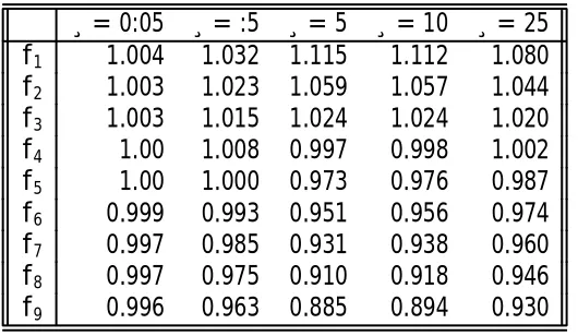
To quantify the di¤erence between the conditional and the unconditional vari-ances we report in Tables 2 and 3 the ratio of the conditional to the unconditional variances, i.e. V ar(rjf)

V ar(r) , for both estimators and for various values of ¸ and f. Speci…cally, for fi, i = 0; :::;10 such that Prffi < f < fi+1g = 0:1; i = 0; :::;9; f0 = 0, f10 = 1. The other parameters have been set at the same values as before, i.e. T = 20, k1 = 3, k2 = 4. Table 2 shows that the di¤erence between V arOLS(rjf) and V arOLS(r) is negligible. On the other hand, Table

3 reinforces the impression gained from Figure 3 that for TSLS the di¤erence between V arT SLS(rjf) and V arT SLS(r) can be very large, especially for small

values of the noncentrality parameter. Notice that small observed values of f

imply, as expected,lower conditional precision for the estimator (relative to the unconditional), but also that larger observed values off implyhigher conditional

precision. It is also clear that for small values of f the conditional precision of

Table 2: Ratio of Conditional to unconditional variance: OLS

¸= 0:05 ¸=:5 ¸= 5 ¸ = 10 ¸= 25

f1 1.004 1.032 1.115 1.112 1.080 f2 1.003 1.023 1.059 1.057 1.044 f3 1.003 1.015 1.024 1.024 1.020 f4 1.00 1.008 0.997 0.998 1.002 f5 1.00 1.000 0.973 0.976 0.987 f6 0.999 0.993 0.951 0.956 0.974 f7 0.997 0.985 0.931 0.938 0.960 f8 0.997 0.975 0.910 0.918 0.946 f9 0.996 0.963 0.885 0.894 0.930

Notes: each entry is calculated as V arOLS(rjf)

V arOLS(r) . Prffi < f < fi+1g= 0:1. T = 20, k1 = 3, k2 = 4, ¯ = 0:35.

Table 3: Ratio of Conditional to unconditional variance: TSLS

¸= 0:05 ¸=:5 ¸= 5 ¸ = 10 ¸= 25

f1 1.821 1.810 1.533 1.365 1.185 f2 1.193 1.196 1.159 1.131 1.078 f3 0.919 0.915 0.974 1.006 1.013 f4 0.746 0.744 0.854 0.919 0.966 f5 0.623 0.625 0.765 0.851 0.927 f6 0.529 0.531 0.691 0.794 0.893 f7 0.451 0.455 0.626 0.742 0.861 f8 0.381 0.385 0.567 0.691 0.828 f9 0.312 0.316 0.503 0.634 0.790

Notes: each entry is calculated as V arT SLS(rjf)

In practice the variance, whether conditional or unconditional, depends on unknown parameters (in the cases of interest here, ¸ and ¯), and the reported

variance is typically calculated by simply replacing these by estimates. The nat-ural (unrestricted maximum likelihood) estimator for ¸ is simply f =2:

Replac-ing ¸ by f=2 in the variance ratios V arOLS(r j f)=V arOLS(r) and V arT SLS(r j

f)=V arT SLS(r) means that these are both functions of ¯2 alone, and ¯ here can

be interpreted as the value of the estimator, rather than the unknown parame-ter. Thus, one can easily examine the e¤ect of conditioning on theestimated, as distinct from the actual, variances of the two estimators. The results of doing so are in broad agreement with the message conveyed in Tables 2 and 3: for the OLS estimator, the ratio of estimated variances always remains close to unity for all values off and ¯;while for the TSLS estimator the ratio can be either much greater than one (when f is small), or much less than one (when f is large).

Thus, the estimated conditional variance continues to re‡ect, more adequately than the estimated unconditional variance, the precision of the TSLS estimator for the sample actually available.

Finally, since both estimators are (conditionally and unconditionally) biased, it is of interest to compare their conditional mean-square-errors, given f. From equations (30) and (31), the di¤erence between the conditional mean-square-errors is:

¢MSE(r_jf) =MSEOLS(rj f)¡M SET SLS(rjf)

= (1_¡w)[4¸¯

2 k2 0

H1(z)¡[w(À ¡2)]¡11H0(z)¡

2¸(1 +w)¯2 wk2(À¡2) 1

H¤

1(z)] (32)

where w = f =(1 +f): Using the contiguity relations for the con‡uent hyperge-ometric function (Abramowitz and Stegun (1965), p.506), this can be expressed entirely in terms of the function1H0. We …nd, after some tedious algebra,

¢MSE(r_jf) = [(1_¡w)(1 +¯2)=w][½2(2 + (1 +w)(k2¡1)

w(À_¡k2¡2)

)

¡1H0(z)

½

½2(2 + (1 +w)(k2¡1)

w(À_¡k2¡2)

) + (1¡½

2₎

(À_¡2) +

2¸½2_{(1 +w)(À¡3)}

(À_¡2)(À_¡k2¡2)

¾

] (33)

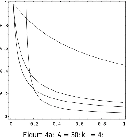
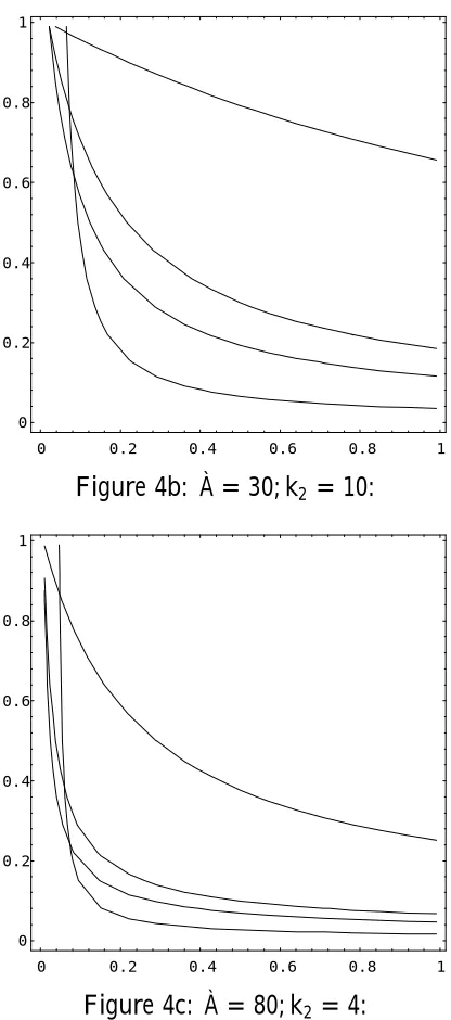
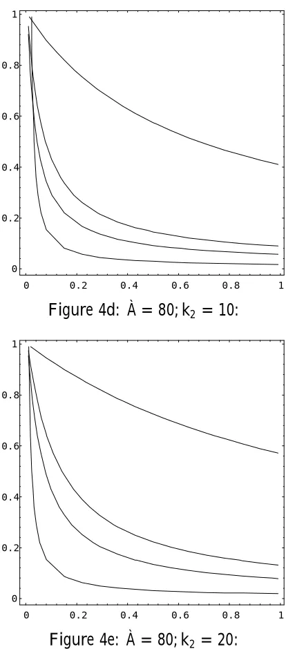
½2 _{= 0, i.e., ¯ = 0, so that OLS conditionally dominates TSLS when there is} no correlation between the right hand side endogenous variable and the error term in the structural equation. Also, it is clear that¢MSE _¡!0 as w _¡! 1 (i:e:; f ¡! 1), so that there is, conditionally, nothing to choose between these

estimators when the sample identi…ability test statistic is large. In Figures 4a -4f we plot conditionalMSEindi¤erence curves (along which¢MSE = 0)in the

(w; ½2_{) plane, for various values of (À; k}

2), and, on each graph, several values of ¸. OLS dominates to the south west of each curve, TSLS to the north east.

Figure 4

Conditional Mean-square-error Indi¤erence Curves: OLS/TSLS

Vertical axis: ½2 _=¯2_{=(1 +¯}2_{); Horizontal axis: w=f=(1 +f)} Plotted for¸ =:05 (top),¸=:5; ¸= 1:0, and ¸= 10 (bottom)

OLS dominates to the south west of each curve.

0 0.2 0.4 0.6 0.8 1 0

0.2 0.4 0.6 0.8 1

0 0.2 0.4 0.6 0.8 1 0

0.2 0.4 0.6 0.8 1

Figure 4b: À = 30; k2 = 10:

0 0.2 0.4 0.6 0.8 1 0

0.2 0.4 0.6 0.8 1

0 0.2 0.4 0.6 0.8 1 0

0.2 0.4 0.6 0.8 1

Figure 4d: À = 80; k2 = 10:

0 0.2 0.4 0.6 0.8 1 0

0.2 0.4 0.6 0.8 1

0 0.2 0.4 0.6 0.8 1 0

0.2 0.4 0.6 0.8 1

Figure 4f: À = 80; k2 = 30:

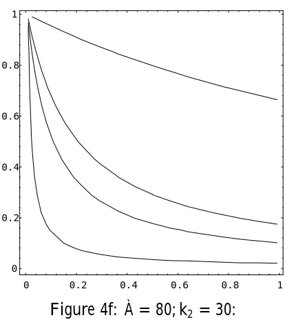
Several important conclusions can be drawn from Figure 4:

(i) In anactually weakly identi…ed model (¸ =:05) OLS dominates TSLS over a large range of (w; ½2_{)values. Even quite strong sample evidence of identi…cation}

(i:e:; a moderate value of f) does not imply superiority of the TSLS estimator.

(ii) If thesample evidence (f)indicates that the model is only weakly identi…ed,

OLS is the preferred estimator.

(iii) The greater the degree of overidenti…cation (k2), the larger the region over which OLS dominates TSLS, but, ceteris paribus, a larger sample size increases the extent of the region over which TSLS dominates.

5 Concluding Remarks

In a single structural equation model the possibility that the model is unidenti…ed, or is arbitrarily close to being unidenti…ed, cannot be ruled out a priori. Even though it is well known that both the small sample and asymptotic properties of the usual estimators break down in such a case, no practical procedure has been developed to take account of this possibility. In this paper we have argued that, in possibly unidenti…ed models, (i) inference should be made conditional on an identi…cation test statistic, and (ii) the identi…cation test statistic should be considered as an index of precision for inference.

We have derived the exact distributions of the OLS and TSLS estimators conditional on an identi…cation test statistic, and shown that conditioning makes the functional forms of the densities of the OLS and TSLS estimators di¤erent. In the extreme case of a totally unidenti…ed model the OLS estimator is independent of the identi…cation test statistic, but that is not the case for the TSLS estimator. The variances of the OLS and TSLS estimators are a¤ected by conditioning more than their means, and, for the TSLS estimator, conditioning can have a substantial e¤ect on the apparent precision of the estimator, in both directions. Conditional mean-square-error comparisons of the two estimators imply that, particularly when the data suggests only weak identi…cation, OLS is the preferred estimator, and that, when properly conditioned, there is little to choose between these two estimators. It would obviously be of interest to include the LIML estimator in these comparisons, but technical problems have so far prevented us from doing so.

6 References

Abramowitz, M., and I.A. Stegun (1965), “Handbook of Mathematical Func-tions”, Dover, N.Y.

Anderson, T.W., K. Morimune and T. Sawa (1983), “The Numerical Values of Some Key Parameters in Econometric Models”, Journal of Econometrics, 21, 229-243.

Barndor¤-Nielsen, O.E. (1980), “Conditionality Resolutions”,Biometrika, 67, 2, 293-310.

Basu, D. (1981), “On Ancillary Statistics, Pivotal Quantities and Con…dence Statements”, in Y.P. Chaubey, and T.D. Dwivedi (eds.),Topics in Applied Statis-tics, Concordia University, Montreal, Reprinted in Gosh (1988).

Cox, D.R. (1958), “Some Problems Connected with Statistical Inference”, The Annals of Mathematical Statistics, Vol. 29, 357-37.

Chikuse, Y. and A.W. Davis (1986), “A Survey on the Invariant Polynomials with Matrix Arguments in Relation to Econometric Distribution Theory”, Economet-ric Theory, 2, 232-248.

Choi, I. and P.C.B. Phillips (1992), “Asymptotic and Finite Sample Distribution Theory of IV Estimators and Tests in Partially Identi…ed Structural Equations”,

Journal of Econometrics, 51, p. 113-150.

Cox, D.R., and D.V. Hinkley (1974), Theoretical Statistics, Chapman and Hall, London.

Creasy, M.A. (1954), “Limits for the Ratio of Means”, Journal of the Royal Statistical Society, Series B, Vol. XVI, 186-194.

Davis, A.W. (1979), “Invariant Polynomials with Two Matrix Arguments Extend-ing the Zonal Polynomials: Applications to Multivariate Distribution Theory”,

Dobrigal, A., D.A.S. Fraser and R. Gebotys (1987), “Linear Calibration and Conditional Inference”, Communications in Statistics, Theory and Methods, 16, 4, 1037-1048.

Dufour, J.-M. (1997), “Some Impossibility Theorems in Econometrics with Ap-plications to Instrumental Variables and Dynamic Models”, Econometrica, Vol. 65, No. 6, 1365-1388.

Efron, B. and D.V. Hinkley (1978), “Assessing the Accuracy of the Maximum Likelihood Estimator: Observed versus Expected Fisher Information,Biometrika, 65, 3, 457-487.

Fieller, E.C, (1954), “Some Problems in Interval Estimation”, Journal of the Royal Statistical Society, Series B, Vol. XVI, 175-185.

Forchini, G. (1998), “Exact Distribution Theory for some Econometric Prob-lems”, Unpublished Ph.D. Dissertation, University of Southampton, January 1998.

Ghosh, J.K. (1988),Statistical Information and Likelihood. A Collection of Crit-ical Essay by Dr. D. Basu, Lecture Notes in Statistics, Springer Verlag.

Gleser, L.J. and J.T. Hwang (1987), “The Nonexistence of 100(1-®) Con…dence

Sets of Finite Expected Diameter in Errors in Variables and Related Models”,

The Annals of Statistics, 15, 1351-1362

Goutis, C. and G. Casella (1995), “Frequentist Post-Data Inference”, Interna-tional Statistical Review, 63, 3, 325-344.

Hillier, G.H. (1985), “On the Joint and Marginal Densities of Instrumental Vari-able Estimators in a General Structural Equation”,Econometric Theory, 1, 53-72.

Hillier, G.H. (1990), “On the Normalization of Structural Equations: Properties of Direction Estimators”,Econometrica, Vol. 58, No. 5, 1181-1194.

Hoadley, B. (1970), “A Bayesian Look at Inverse Linear Regression”,Journal of the American Statistical Association, Vol. 65, No 329, 356-369.

James, A.T. (1954), “Normal Multivariate Analysis and the Orthogonal Group”,

The Annals of Mathematical Statistics, 25, 40-75.

James, A.T., G.N. Wilkinson and W.N. Venables (1974), “Interval Estimates for a Ratio of Means”,Sankhy¯a, Vol. 36, Series A, Pt. 2, 177-183.

Koschat, M.A. (1987), “A Characterization of the Fieller Solution”,The Annals of Statistics, Vol. 15, No. 1, 462-468.

Lindsay, B.G. and B. Li (1997), “On Second-Order Optimality of the Observed Fisher Information”,The Annals of Statistics, Vol. 25, No. 5, 2172-2199.

Muirhead, R.J. (1982),Aspects of Multivariate Statistical Theory, John Wiley & Sons, Inc., New York.

Phillips, P.C.B. (1983), “Exact Small Sample Theory in the Simultaneous Equa-tion Model”, in M.D. Intriligator and Z. Griliches, eds.,Handbook of Economet-rics, Amsterdam: North Holland.

Phillips, P.C.B. (1989), “Partially Identi…ed Econometric Models”,Econometric Theory, 5, 181-240.

Sche¤é, H. (1970), “Multiple Testing versus Multiple Estimation. Improper Con-…dence Sets. Estimation of Directions and Ratios”,The Annals of Mathematical Statistics, Vol. 41, No.1, 1-29.

Sims, C.A. (1980), “Macroeconomics and Reality”, Econometrica, Vol. 48, No. 1, 1-48.

Staiger, D. and J.H. Stock (1997), “Instrumental Variables Regression with Weak Instruments”. Econometrica, Vol. 65, No. 3, 557-586.

APPENDIX A: Conditional Densities

In this Appendix we make extensive use of the notation and multivariate integration techniques explained in detail in Muirhead (1982), especially Chapters 2 and 7. To keepthe derivations as brief as possible, we ask the reader to refer to these sources for details of the notation and main results that are used. See also Hillier (1985), and Hillier and Skeels (1993).

Let

X = (Z₂0PZ1Z2)

1 2¦^

2-¡

1 2

22 ; M = E(X) = (Z₂0PZ1Z2)

1 2¦₂-¡

1 2

22 ; and R = -¡12

22 S22-¡

1 2

22 : The maximal invariant for the testing problem of interest consists of thencharacteristic roots ofF0 in equation (14) in the text, or, equiva-lently, ofF =R¡12X0XR¡12. SinceX»N(M; I_k2-I_n);andR »W_n(À¡k₂; I_n),

and X and R are independent, the marginal joint density of the roots of F is

given by Muirhead (1982), Theorem 10.4.2 as:

pdf(F) =C2etrf¡¤g jFj k₂

2 ¡pjI

n+Fj¡

À

2

1F1(n)( À

2;

k2

2; ¤; F(In+F)

¡1₎Y

i<j

(fi¡fj)

(A1) where¤ = 1₂M0M, F =diagff1; f2; ::::; fng, and

C2 =

¼n22¡_n(À

2)

¡n(n₂)¡n(À¡₂k2)¡n(k2₂)

:

Note that here and below we use F to denote both the original matrix variate, and the diagonal matrix containing the characteristic roots of that matrix. This, we hope, will economise on notation without confusing the reader too much.

Using the de…nitions ofrand¯in (5) and (6) in the text, and the assumptions

made in Section 3, it is straightforward to check that:

rOLS jX; R sN((R+X0X)¡1X0M ¯;(R+X0X)¡1); (A2)

and

rT SLS jX sN((X0X)¡1X0M ¯;(X0X)¡1): (A3)

any parameters of the model. Hence, unconditionally, the densities of rOLS and

rT SLS are independent of the model parameters, and those of the unstandardised

bOLS andbT SLS depend only on -; as noted in the introduction.

From (A2) and (A3), it is straightforward to obtain the joint density of

(r; X; R) for both of these estimators. To obtain the joint density of (r; F)

in both cases we need to transform to a set of new variates including(r; F), and then integrate out the redundant variables. We have, as the starting points:

pdf_OLS(r; X; R) =C1etrf¡¤g jRj À¡k₂

2 ¡pjR+X0Xj 1

2 etrf¡1

2(R+X

0_X)(I

n+rr0)g

etrfX0M(In+¯r0)gexpf¡

1 2¯

0_M0_X(R+X0_X)¡1_X0_{M¯g; (A4)}

and

pdfT SLS(r; X; R) =C1etrf¡¤g jRj À¡k2

2 ¡pjX0Xj 1

2_etrf¡1

2Rgetrf¡ 1 2X

0_X(I

n+rr0)g

etrfX0M(In+¯r0)gexpf¡

1 2¯

0_M0_X(X0_X)¡1_X0_{M¯g; (A5)}

wherep= (n+ 1)=2 and

C1 = [(2¼) n(k2+1)

2 2

n(À¡k2)

2 ¡_n(À¡k2

2 )]

¡1_:

Conditional density of the OLS estimator

We deal with the OLS case, equation (A4), …rst. The characteristic roots of F

are invariant under the transformations X _¡!KXP H; R _¡!H0_P0_{RP H; with}

K ₂ O(k2); P 2 Gl(n); and H 2 O(n). Choosing P = (In +rr0)¡ 1

2, making

these transformations in (A4) (the Jacobian is (1 +r0r)¡k2+2n+1), and averaging

overO(k2) andO(n), the joint density in (A4) is replaced by:

C1etrf¡¤g(1 +r0r)¡

(À+1) 2 jRj

(À¡k₂₎

2 ¡pjR+X0Xj 1

2 _etrf¡1

2(R+X

0_X)g 1

X

j:k=0

X

®;[k];Á

C_Á®;[k](1

2M GG0M0;¡ 1 2M ¯¯

0_M0_)C®;[k]

Á (12XX0; X(R+X0X)¡ 1_X0₎

j!k!(n

2)®CÁ(Ik2)

;

(A6)

where we have temporarily put G = (In+¯r0)(In+rr0)¡ 1

2; and we have made