TRINITY COLLEGE DUBLIN
C
OL
AISTE NA
´
TR´
ION
OIDE, BAILE
´
´A
THA
C
LIATH
First-Order Reasoning for Higher-Order
Concurrency
Vasileios Koutavas
Matthew Hennessy
First-Order Reasoning for Higher-Order Concurrency
∗
Vasileios Koutavas
Matthew Hennessy
{Vasileios.Koutavas, Matthew.Hennessy}@cs.tcd.ie
Trinity College Dublin
July 23, 2009
Abstract
By combining and simplifying two of the most prominent theories for HOπof San-giorgi et al. and Jeffrey and Rathke [15, 4], we present an effective first-order theory for a
higher-orderpicalculus.
There are two significant aspects to our theory. The first is that higher-order inputs are treated in a first-order manner, hence eliminating the need to reason about arbitrarily complicated higher-order contexts, or to use up-to context techniques, when establishing equivalences between processes. The second is that we use augmented processes to record directly the knowledge of the observer. This has the benefit of making ordinary first-order weak bisimulation fully abstract w.r.t. contextual equivalence. It also simplifies the handling of names, giving rise to a truly propositional Hennessy-Milner characterisation of higher-order contextual equivalence.
Furthermore, we illustrate the simplicity of our approach in proving several interesting equivalences by exhibiting first-order witness weak bisimulations, and inequivalences by using the propositional Hennessy-Milner Logic. Finally we show that contextual equiva-lence in a higher-order setting is a conservative extension of the first-orderpicalculus.
Contents
1 Introduction 3
2 The Language 5
2.1 Syntax . . . 5 2.2 Reduction semantics . . . 7 2.3 A behavioural equivalence . . . 8
3 The Labelled Transition System 9
4 Bisimulations 15
4.1 Strong Bisimulations . . . 15 4.2 Weak Bisimulations . . . 15 4.3 Logical Characterisation . . . 17
5 Soundness of Weak Bisimilarity 20
6 Completeness of Weak Bisimilarity 31
6.1 Concretion of Configurations . . . 31
6.2 Completeness . . . 33
7 Full Contextual Equivalence 36 8 Examples 39 8.1 Implementation of Replication . . . 40
8.2 A Trigger-Installing Ping Service . . . 42
8.3 A Trigger-Promoting Ping Service . . . 43
8.4 Composition of Triggers with Replication . . . 44
8.5 The Processes in Figure 1 . . . 46
9 First-Order Processes 49
c?(X,Y).νt.!c!"(appX⊕appY)|appX$.0⊕c!"t!.appY$.0"| ∗(t?.(appX⊕appY) ) ?
≈c?(X,Y).νt.!c!"(appX⊕appY)|appY$.0⊕c!"t!.appX$.0"| ∗(t?.(appX⊕appY) ) (†)
c?(X,Y).νt.!c!"(appX|appY)⊕appX$.0⊕c!"t!.appY$.0"| ∗(t?.(appX|appY) )
?
≈c?(X,Y).νt.!c!"(appX|appY)⊕appY$.0⊕c!"t!.appX$.0"| ∗(t?.(appX|appY) )
(‡)
Figure 1: An Equivalence and an inequivalence in higher-order concurrency
1 Introduction
Developing effective reasoning techniques for languages with higher-order constructs is a challenging problem, made even more challenging with the presence of concurrency and mo-bility. The difficulties involved are exemplified by the search for reasonable proof techniques for establishing behavioural equivalences between processes written in higher-order versions of thepicalculus, [11, 12, 13, 15, 16]. The picalculus is an abstract process description language in which first-order values are exchanged between sub-processes using communi-cation channels. Much of its power derives from the fact that these values include the set of communication channels, which can be generated dynamically and shared privately among sub-processes. Higher-order versions also allow processes, or some form of abstractions over processes, to be communicated; that is the values communicated may be higher-order.
Intuitively two processes are deemed to be behaviourally equivalent if no user in any context can distinguish between them [10]; this has been formalised for a wide range of languages, including the higher-orderpicalculus, called HOπ, and is often referred to as con-textual equivalence[3, 4, 5]; a slight variation is calledbarbed congruence[16, 12, 11]. The challenge is to develop useful reasoning techniques for this contextual equivalence, in partic-ular techniques which do not involve reasoning about all possible programming contexts.
To illustrate the challenges of reasoning in higher-order concurrent languages let us con-sider the pairs of higher-order processes shown in Figure 1, where⊕is an internal choice operator andapp causes the execution of asuspended process. The differences within each pair of processes is highlighted. All processes initially receive two suspended processesX andY on channel c and dynamically create a local channel t. Then, each one combines theX andY in a slightly different way into two possible replies on channelc, chosen non-deterministically. After a reply is sent, all it is left of the processes is the same replication (denoted by the∗-operator) guarded by the private channelt. Up to this point the behaviour of the processes is indistinguishable by a potential interrogator. But from this point on the interrogator may use the values previously emitted from the processes to make further obser-vations. These include replication and execution of the values, as well as their embedding in more complex values fed into other instances of the same processes.
Our aim is to develop a practical and effective reasoning methodology for such processes. Our methodology will only employ first-order reasoning and we will see that the examples in Figure 1 can be handled in a straightforward manner.
thepicalculusand related languages the relevant actions take the form
output:P(ν−→n)c!V P( input : P(ν−→n)c?V P( (1)
HerePis the process under investigation, P(the result of the investigation,ca
communi-cation channel,V an acceptable value which may be higher-order, andnrepresents the new informationextrudedby the process under investigation to the interrogator. These actions are defined using a Labelled Transition System (LTS), and then roughly speakingPandQare deemed equivalent whenever they can support the same possible interrogations.
A number of different formulations of bisimulations have been developed for HOπ includ-ingnormal bisimulation[11, 12], and its abstract version in [4], andenvironmental bisimula-tions[15]. All have been shown to coincide withcontextual bisimulation[13] (often referred to as beingfully-abstract) but we believe that none have provided a satisfactory applicable proof technique for program equivalence; as evidence we can cite the near complete lack of examples in the research literature. The aim of the current paper is to design an elementary bisimulation theory which is not onlyfully-abstractwith respect to contextual equivalence but also supports a reasonable proof methodology, one in which program equivalence can be readily exhibited. By a careful selection of ideas from [4] and [15], together with the combination and simplification of their formalisms, we will end up with a purely first-order theory of bisimulations in which actions take a particularly simple form, and in which wit-ness bisimulations underlying equivalences between higher-order processes are very easy to describe.
Sangiorgi et al. [15], motivated by work in sequential languages [19, 18, 7, 6, 8], use an LTS with the actions in (1) above and annotate bisimulations with an environment (relation) containing the knowledge currently known to the interrogator; this allows the interrogating actions to be meaningfully based on the interrogator’s current knowledge. Their method simplifies the metatheory (e.g. showing that bisimilarity is a congruence), but leads to a definition for bisimulations with many and arguably complex conditions. As an example, for higher-order inputs of related processes one has to consider all possiblerelated, and not just identical, input values.
Let us briefly explain this point. Knowledge about two potentially bisimilar processes is accumulated by the interrogator by storing all (higher-order) values output by the processes in the knowledge environment. This knowledge can subsequently be used to construct arbitrarily complicated new values with which to further interrogate the processes. It is this generation of arbitrary new values, using knowledge previously gleaned from the process, which accounts for the requirement to quantify over all related contexts. This strong proof obligation is sometimes mitigated by the use of up-to context techniques.
Jeffrey and Rathke [4] use a more restrictive approach offormal triggers. A higher-order output of a process is transformed to a special trigger service holding the actual value and only a pointer for invoking the service is passed to the interrogator. Similarly, a higher-order input is fed with a trigger with which the process can intuitively run the actual value—but actually only an observable action is recorded in the LTS.
We believe that both methods have useful intuitions and that their combination has greater value than the sum of its parts. Hence our theory combines and simplifies their insights. We use knowledge environments in the LTS that record the values exposed to the context, and test related processes with symbolic higher-order inputs. In this way we recover a representation of triggers similar to [4], together with an explicit record of the names that are known to the context.
• the (higher-order) process under interrogationP,
• a representation ∆of the knowledge currently known to the interrogator about this process,
• the informationaknown to the process but currently unknown to the interrogator. This extension allows us to simplify considerably the actions on which our bisimulations are based; in particular it eliminates the need for explicitlyextrudingnew information. Thus the actions in (1) above, now applying to configurations, are labelled simplyc!vandc?v respectively, thereby relieving us of the need to manage the complications inherent in the use of extrusion. A significant consequence is that bisimulation in our theory is characterised by a propositionalHennessy-Milner Logic (HML) [2], that would not be possible by using Jeffrey and Rathke’s LTS.
The main contributions of the paper can be summarised as follows:
(i) We define a first-order, fully-abstract, theory of standard weak bisimulation equivalence for a higher-orderpicalculus, called pp-π, that unifies two distinct techniques. The the-ory is compositional in the sense that the equivalence is preserved by arbitrary process contexts.
(ii) The associated coinductive reasoning technique for pp-πprocesses is effective; because the theory is first-order it is straightforward to demonstrate equivalences between pro-cesses by exhibiting witness bisimulations. In support of this we provide a series of compelling example process equivalences, which the literature of higher-order concur-rency currently lacks.
(iii) We give the first propositional HML characterisation of weak bisimulation for a higher-orderpicalculus; this result easily transfers to the first-orderpicalculus. We use this to give simple proofs ofinequivalence between higher-order processes, which is difficult to achieve with existing theories.
(iv) We prove that contextual equivalence in a higher-order setting is a conservative exten-sion of the first-orderpicalculus, thus confirming that results and reasoning methods from first-orderpicalculustransfer to a higher-order setting.
The remainder of the paper is organised as follows: the next section defines the language pp-π, giving the syntax, a reduction semantics and a simple type system for ensuring that com-municated values are appropriately typed. Section 3 details our first-order LTS for pp-π, and Section 4 defines strong and weak bisimulations and a characterisation of the latter in terms of a propositional Hennessy-Milner Logic. Sections 5 and 6 contain the proofs of soundness and completeness of our theory with respect to contextual equivalence that preserves only parallel contexts, and Section 7 proves that our theory is fully abstract with respect to the full contextual equivalence. Section 8 is devoted to proving several interesting equivalences by using weak bisimulations, and an inequivalence by providing a discriminating HML formula. Section 9 proves the conservativity theorem; the paper closes in Section 10 with conclusions and a discussion of related work.
2 The Language
2.1 Syntax
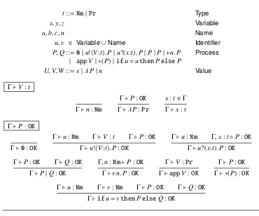
t::=Nm|Pr Type
x,y,z Variable
a,b,c,n Name
u,v ∈ Variable∪Name Identifier
P,Q::=0|u!"V:t$.P|u?(x:t).P|P|P|νn.P Process
| appV | ∗(P)|ifu=uthenPelseP
U,V,W ::=x|λP|n Value
Γ+V:t
Γ+n:Nm
Γ+P:OK
Γ+λP:Pr
x:t∈Γ Γ+x:t
Γ+P:OK
Γ+0:OK
Γ+u:Nm Γ+V:t Γ+P:OK
Γ+u!"V:t$.P:OK
Γ+u:Nm Γ,x:t+P:OK
Γ+u?(x:t).P:OK
Γ+P:OK Γ+Q:OK
Γ+P|Q:OK
Γ,n:Nm+P:OK
Γ+νn.P:OK
Γ+V:Pr
Γ+appV:OK
Γ+P:OK
Γ+ ∗(P) :OK
Γ+u:Nm Γ+v:Nm Γ+P:OK Γ+Q:OK
[image:8.595.110.480.102.410.2]Γ+ifu=vthenPelseQ:OK
Figure 2: Syntax and typing of pp-π
assume a set of channel namesName, ranged over by a,b, . . . and a separate set of vari-ablesVariable, ranged over byx,y, . . ., and useu,v, . . .to denote identifiers, from (Variable∪
Name).
The basic constructs in pp-π are the input and output of typed values along channels, u?(x:t).Pandu!"V:t$.P. In the former a value of typetis received on channeluand bound to the variablexinP, while in the latter the valueV of typet is output on channelu and the process continues with the execution of the codeP. In addition we have the standard constructs of thepicalculus: replication ∗(P), parallel execution (P|Q), the generation of new namesνn.P, and the testing of these namesifu=vthenPelseQ.
In thepicalculusthe only values which can be transmitted along channels are names, but in pp-πthunkedorsuspendedprocesses, of the formλP, are also allowed; when such a value is received by a process it can be executed, via the new constructappV.
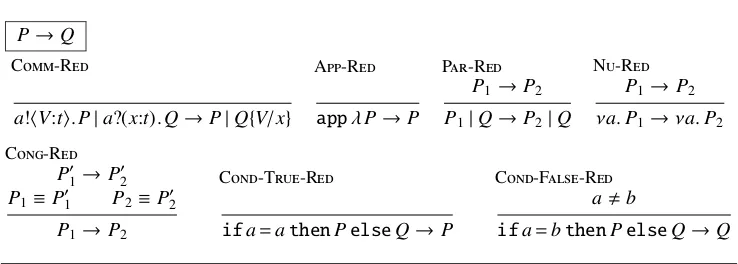
P→Q
C-R
a!"V:t$.P|a?(x:t).Q→P|Q{V/x}
A-R
appλP→P
P-R
P1→P2
P1|Q→P2|Q
N-R
P1 →P2
νa.P1 →νa.P2
C-R
P(
1→P(2
P1 ≡P(1 P2≡P(2
P1→P2
C-T-R
ifa=athenPelseQ→P
C-F-R
a"b
[image:9.595.113.482.106.238.2]ifa=bthenPelseQ→Q
Figure 3: Reduction semantics for pp-π
Typing: We have a very-lightweight notion of type whose purpose is simply to ensure, dy-namically, that at any point in time when a value is received at a certain type it is subsequently only used at that type. Values can be one of two types,Nmfor names andPrfor (suspended)
processes. Type inference is with respect totype environments, consisting of finite sets of variable-type associationsx:t. Then the typing judgements take the form
• Γ+V:t, indicating that relative toΓthe valueVhas typest
• Γ+P:OK, indicating that the process termPis well-typed relative toΓ.
The rules for inferring the judgements are also given in Figure 2.
Example: Consider the following process, which describes a service ats:
∗(s?(x:Nm).s?(y:Pr).νf. νr.x!"f$.x!"r$.
∗(f?(z:Nm).z!"y:Pr$.0)| ∗(r?.appy))
It first receives as input a reply channel name, bound tox, and then a (suspended) process bound toy. It generates two new names f andrwhich it returns on the reply channel, and then sets up two new servers at those names. The first, atf, receives a name and forwards the suspended process there; the second, atr, runs the suspended process on request.
Notice that we do not assume any static typing for channel names. At different points in time they may be used to communicate values of different type. So, for example, a client using this service atswill be expected to follow an implicit protocol, whereby first a name is sent onsand then a process.
2.2 Reduction semantics
This is expressed as a relation
P→Q
wherePandQare assumed to be well-typed processes, that is process terms satisfying∅ +
P:OKand∅ +Q:OK. The rules for inferring these judgements are given in Figure 3, and are
Note that this communication alongacan only happen if the partners agree on the type of the value being transmitted. The other significant rule is for the initiation of a suspended process,
appλP→P
The remaining rules are standard, borrowed from thepicalculus; in particular reductions are relative to a structural equivalenceP≡Qwhich we now define.
Definition 2.1(Structural equivalences). Limited structural equivalence ( ˆ=)is defined to be the least equivalence relation on processes satisfying the axioms
P=0|P P|Q=Q|P (P1|P2)|P3=P1|(P2|P3) and closed under the two operators− |− andνa.−.
Structural equivalence(≡)is obtained by adding the further axioms
νa. νb.P=νb. νa.P ∗(P)=P| ∗(P) νa.0=0 νa.(P|Q)=(νa.P)|Q (a!fn(Q))
As we have already stated, structural equivalence (≡) is used in the reduction semantics, but the more restrictive limited equivalence ( ˆ=) will be useful in proofs of equivalence. Lemma 2.2(Substitution). IfΓ,x:t+P:OKand+V:t thenΓ+P{V/x}:OK.
Proof. By rule induction. !
Lemma 2.3. IfΓ,x:t+P:OKand x!fn(P)thenΓ+P:OK.
Proof. By rule induction. !
Lemma 2.4. If P≡Q andΓ+P:OKthenΓ+Q:OK.
Proof. By case analysis on Definition 2.1, using Lemma 2.3. !
Proposition 2.5(Preservation). If+P:OKand P→Q then+Q:OK.
Proof. By rule induction onP→Q, using Lemmas 2.2 and 2.4. !
2.3 A behavioural equivalence
We focus on reasoning about contextual equivalence [4, 5, 16, 12, 11] of closed, well-typed processes, but in this section we content ourselves with a simplified version of it. We write P R P(whenRis a binary relation on closed, well-typed processes and (P,P()∈R.
We consider the basic observable of a process to be the ability to output on a given chan-nel, called a barb.
Definition 2.6(Barbs). We write P↓bif and only if there exist c,V,t,P1,P2, with b!{c}, such
that P≡νc.(b!"V:t$.P1|P2).
We write P⇓bif and only if there exists Q such that P→∗Q and Q↓b.
Definition 2.7(Parallel Contextual Equivalence (#pcxt)). (#pcxt) is the largest relation on
closed processes that preserves barbs, is reduction closed, and is preserved by parallel con-texts; i.e. P#pcxt P(if and only if
(ii) Reduction closed: for all P1 with P → P1 there exists P(1 such that P( →∗ P(1 and
P1#pcxtP(1, and vice-versa, and
(iii) Preserves parallel constructs:for all well-typed processes Q, P|Q#pcxtP(|Q.
It is straightforward to show that#pcxtis an equivalence relation. On the other hand to give
a direct proof that two processes are related is very difficult, especially in the higher-orderπ -calculus. In the following sections we define a labelled transition system (LTS) and show that (#pcxt) coincides with weak bisimulation in the LTS. We also demonstrate the usefulness of
bisimulation as a proof technique of equivalence via several examples. Finally we show that the equivalence remains unchanged if we extend the third requirement (3) to demand that the relation be preserved by all contexts.
3 The Labelled Transition System
The idea behind an LTS-based semantics for a process language is to describe the interactions which an observer can have with processes; indeed semantic equivalences such as bisimula-tion equivalence can be expressed in terms of games, and strategies for such games, over these interactions [17].
We first give an informal account of the kinds of interactions we envision for pp-πand then consider their formalisation. For the standard (first-order)picalculusobservers interact with processes via inputs and outputs on channels. But these interactions are constrained by the knowledge which the observer has of the process being interrogated. For example if an observer has no knowledge of channelbthen it can not distinguish between the two processes
a!.0|b!.0 a!.0
as the only possible known source of interaction is the channela.
In general the observer’s knowledge is accumulated by receiving values from the process under interrogation. In pp-π the observer also accumulates knowledge about higher-order values, and may use these to further interrogate the process. This further interrogation can either take the form of transmitting these values along communication channels orexecuting them. For example consider the two processes
Pdef= νa.c!"λa!.0$.a?.0 Qdef= νa.c!"λa!.0$.a?.c!.0
and an observer which only knows of the channelc. By inputting oncit gains knowledge of the (suspended) processa!.0although it does not gain any knowledge of the existence of the private channela. Nevertheless by running this suspended process a difference can be detected betweenPandQ; in one case output can be detected on channelcafter the execution
of the suspended process.
However, even in the first-order case, it is necessary for the observer to independently generate new values with which to interrogate the process. For example consider a situation in which the observer is only aware of the channel namea. Then the only way for the observer to distinguish between the two processes
a?(x).0 a?(x).ifx=athen 0 elsea!.0
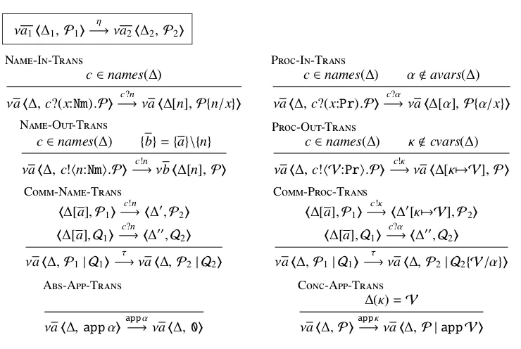
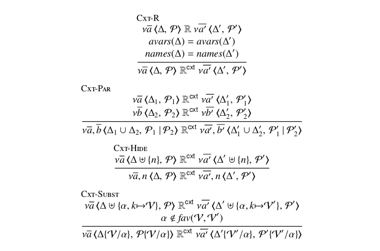
νa1!∆1,P1"
η
−→νa2!∆2,P2"
N-I-T
c∈names(∆)
νa!∆,c?(x:Nm).P"−→c?n νa!∆[n],P{n/x}"
P-I-T
c∈names(∆) α!avars(∆)
νa!∆,c?(x:Pr).P"−→c?α νa!∆[α],P{α/x}"
N-O-T
c∈names(∆) {b}={a}\{n}
νa!∆,c!"n:Nm$.P"−→c!n νb!∆[n],P"
P-O-T
c∈names(∆) κ!cvars(∆)
νa!∆,c!"V:Pr$.P"−→c!κ νa!∆[κ0→V],P"
C-N-T
!∆[a],P1"
c!n
−→!∆(,P2"
!∆[a],Q1"
c?n
−→!∆((,Q2"
νa!∆,P1| Q1"
τ
−→νa!∆,P2| Q2"
C-P-T
!∆[a],P1"
c!κ
−→!∆([κ0→V],P2"
!∆[a],Q1"
c?α
−→!∆((,Q2"
νa!∆,P1| Q1"
τ
−→νa!∆,P2| Q2{V/α}"
A-A-T
νa!∆,appα"app−→ανa!∆,0"
C-A-T
∆(κ)=V
[image:12.595.114.484.106.354.2]νa!∆,P"app−→κνa!∆,P |appV"
Figure 4: The LTS: main rules (omitting symmetric rules)
higher-order values are simply abstract variables, ranged over byα, taken from a count-able setAVariables, which is assumed to be disjoint from the ordinary program variables
Variables. On receiving such an abstract higher-order valueαthe processes under interroga-tion has very little it can do with it;αcan only be transmitted as a value along other channels. However, as we will see, our LTS will also allow the process to applyαin a trivial manner. To accommodate these abstract values we need to extend the syntax in Figure 2 to allow them to be used as values. We letPandVrange over the extended syntax ofabstractprocesses,
AProcess, andabstractvalues,AValue, respectively;fav(P) denotes the set of abstract vari-ables occurring inP. Furthermore we extend the typing rules to apply to abstract processes and values by adding the following typing judgement for abstract variables:
Γ+α:Pr
In order to formalise these kinds of interactions our LTS needs to take into account both the process being interrogated and the current knowledge of the observer, or context. As we have indicated this knowledge is accumulated via interactions with the process, and consists either of (first-order) channel names or higher-order values. To tabulate the latter we use a countable set ofconcretevariablesCVariable, disjoint from other kinds of variables, and ranged over byκ.
Definition 3.1(Knowledge environments). A knowledge environment∆is a finite set of the kind
Name∪AVariable∪(CVariable→finAValue)
with the property that it maps concrete variables to abstract values of typePr:
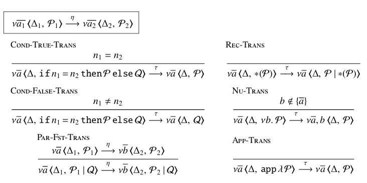
νa1!∆1,P1"
η
−→νa2!∆2,P2"
C-T-T
n1=n2
νa!∆,ifn1=n2thenPelseQ"−→τ νa!∆,P"
R-T
νa!∆,∗(P)"−→τ νa!∆,P | ∗(P)"
C-F-T
n1"n2
νa!∆,ifn1=n2thenPelseQ"
τ
−→νa!∆,Q"
N-T
b!{a}
νa!∆, νb.P"−→τ νa,b!∆,P"
P-F-T
νa!∆1,P1"
η
−→νb!∆2,P2"
νa!∆1,P1| Q"
η
−→νb!∆2,P2| Q"
A-T
[image:13.595.112.478.104.287.2]νa!∆,appλP"−→τ νa!∆,P"
Figure 5: The LTS: more rules (omitting symmetric rules)
We write∆[e] for∆∪{e}, and∆(κ)=Vfor (κ,V)∈∆; we also writenames(∆),avars(∆), andcvars(∆) for the name component, the abstract variable component, and the domain of the functional component of∆, respectively.
Our LTS will be defined betweenconfigurationsof the formνa!∆,P", whereaare names the scope of which extends toPand the processes indexed in∆,Pis an abstract process and ∆is a knowledge environment. Configurations are identified up to alpha-equivalence, are ranged over byC, and are subject to the following well-formedness constraints:
Definition 3.2(Well-Formed Configuration). Awell-formedconfiguration is any configura-tionνa!∆,P"with the properties:
(i) a are distinct bound names
(ii) {a} ∩names(∆)=∅
(iii) +P:OKand fn(P)⊆ {a} ∪names(∆)and fav(P)⊆avars(∆)
(iv) +V:Prand fn(V)⊆ {a}∪names(∆)and fav(V)⊆avars(∆)for everyVin the codomain of∆.
In a configurationνa!∆,P"the environment∆represents the knowledge of the observer. The namesa are those known to the process under investigationP, which are not known to the observer, motivating condition (i); note however that these private names are shared between the process and the abstract values indexed in∆, values sent to the observer from the process. The remaining conditions guarantee that all processes and values must be well-typed and only use names which are inaor are known to the environment, and abstract variables in ∆.
The judgements for the LTS take the form
νa!∆,P"−→η νb!∆(,Q"
(i) Internal action,τ:these are the unobservable actions of the process (e.g. internal com-munication). They weakly correspond to the reduction semantics of Figure 3.
(ii) First-order input, c?n:input by the process along the channelc, known to the observer, of the namen; n might already be known to the observer or is freshly generated—in both casesnis in the knowledge of the observer after the transition.
(iii) Higher-order input, c?α:input by the process of an abstract higher-order nameα. For these actions, αis always taken to be fresh; that is a new abstract name, implicitly freshly generated by the observer.
(iv) First-order output, c!n:output by the process along the channelcof the namen. Here the channelcmust be known to the observer, but the namenmay be a private to the process or known to the observer. In both cases,nis known to the observer after the transition.
(v) Higher-order output, c!κ:output by the process of some value along the channelc. The channelcmust be known to the observer, butκis fresh. Here the actual value output by the process is not represented directly in the label. Instead it is stored in the the knowledge environment∆under the fresh keyκ.
(vi) Abstract value application,appα: the execution by the process of the abstract higher-order valueαsupplied by the observer. But since this is an abstract value, this execution is effectively a noop.
(vii) Concrete value application,appκ: the execution of the higher-order value associated withκin the knowledge environment. This value was originally supplied by the process.
Rules N-I-Tand P-I-Tin Figure 4 capture first-order and higher-order
input of the process, respectively. In the former the observer provides to the process a known or fresh name over a known channel. In the latter the observer provides a new abstract vari-able, representing an arbitrary higher-order value, over a known channel.
Similarly, N-I-Tand P-I-Tcapture first-order and higher-order output
of the process. In the latter, the higher-order value is not sent to the observer. Instead, it is indexed by a new concrete variable, and that variable is sent to the observer.
Rules P-I-Tand P-O-Tinclude a freshness condition for the involved
abstract and concrete variable, respectively, to ensure that abstract variables from distinct input transitions and concrete variables from distinct output transitions are not confused.
Internal communication is captured by C-N-T, for first-order values, and
C-P-Tfor higher-order values. Such communication can take place over
chan-nels that are local to the process, hence the temporary addition of the local chanchan-nels in∆in the premises. Note that in C-P-T, the concrete variableκused to store the value being communicated is not included in the environment∆in the conclusion.
Application of higher-order values is encoded in the rules C-A-Tand A-A
-T. The former says that for the observer to run a value originally supplied by the process,
it simply executes it in parallel with the process currently under observation. In contrast, rule A-A-Tsays that the effect of the process executing an abstract value originally supplied by the observer is simply a signal to the observer (via the label of the transition) and the generation of the empty process0.
The rest of the rules in Figure 5 are mostly house-keeping in nature. The LTS preserves well-formedness of configurations.
(i) ∆1⊆∆2
(ii) νb!∆2,Q"is well-formed.
Proof. By induction on the transitionνa!∆1,P"
η
−→νb!∆2,Q". !
For the remainder of this paper we consider only well-formed configurations.
For the rest of this subsection we analyse in considerable detail the structure of the actions in the LTS. First we give an exhaustive analysis of the structure of configurations which are produced by these actions.
Proposition 3.4. The following properties are true.
(i) Ifνa!∆1,P"
c!n
−→νb!∆2,Q"then for someP1andP2
P=ˆ c!"n$.P1| P2 Q=ˆ P1| P2 ∆2= ∆1[n] {b}={a}\{n}
(ii) Ifνa!∆1,P"−→c!κ νb!∆2,Q"then for someP1andP2
P=ˆ c!"V$.P1| P2 Q=ˆ P1| P2 ∆2= ∆1[κ0→V] {b}={a}
(iii) Ifνa!∆1,P"−→c?n νb!∆2,Q"then for someP1andP2
P=ˆ c?(x:Nm).P1| P2 Q=ˆ P1{n/x} | P2 ∆2= ∆1[n] {b}={a} (iv) Ifνa!∆1,P"−→c?α νb!∆2,Q"then for someP1andP2
P=ˆ c?(x:Pr).P1| P2 Q=ˆ P1{α/x} | P2 ∆2= ∆1[α] {b}={a}
(v) Ifνa!∆1,P"app−→ανb!∆2,Q"then for someP1
P=ˆ appα| P1 Q=ˆ P1 ∆1= ∆2 {b}={a} (vi) Ifνa!∆1,P"app−→κνb!∆2,Q"then for someV= ∆1(κ)
Q=ˆ appV | P ∆1= ∆2 {b}={a} (vii) Ifνa!∆1,P"−→τ νb!∆2,Q"then∆1= ∆2and{a} ⊆{b}.
Proof. All properties are shown by induction on the rules of the LTS. !
In a configurationνa!∆,P"there are two sources of knowledge, the environments knowl-edge in∆and the internal knowledge of the process ina. The next result shows that changes to this knowledge has no effect on many actions.
Proposition 3.5.
(i) Knowledge extension: If νa!∆1,P" −→η νb!∆2,Q" and νa,c!∆03∆1,P" is well-formed, and names(η)∩names(∆0)=avars(η)∩avars(∆0)=cvars(η)∩cvars(∆0)=∅ then
(ii) Knowledge restriction: If νa,c!∆0 3∆1,P" −→η νb!∆03∆2,Q"and νa!∆1,P"is well-formed, andη!{appκ|κ∈∆0} ∪{c?n|n∈∆0}then
νa!∆1,P"
η
−→νb(!∆2,Q"
where{b(}={b}\{c}.
Proof. In both cases we use rule induction on the inference of the actions. !
Information inνa!∆,P"can also be shifted between the observers knowledge∆and the processes knowledgeawithout affecting actions, provided of course that information is not used in the actions.
Proposition 3.6(Unused Information).
(i) Hiding:Supposeνa!∆1[b],P"−→η νd!∆2[b],Q"and b does not occur inη. Then νb,a!∆1,P"
η
−→νb,d!∆2,Q"
(ii) Revealing:Conversely, supposeνb,a!∆1,P"−→η νb,d!∆2,Q"where again b does not occur inη. Then
νa!∆1[b],P"
η
−→νd!∆2[b],Q"
Proof. Again by rule induction. !
With reference to this proposition there are actually very limited ways in which an action ηfrom the configurationνb,a!∆1,P"can use the nameb. Indeed the only possibility is an output action, which by Proposition 3.4 must have the formνb,a!∆,P" −→c!b νd!∆[b],Q"; and this action can still be performed when the observer knows of the existence ofb: Proposition 3.7(Extrusion). Provided c is different than b,
νb,a!∆,P"−→c!b νd!∆[b],Q" iff νa!∆[b],P"−→c!b νd!∆[b],Q"
Proof. By rule induction, in both directions. !
Abstract variables are significant only in application and communication actions that men-tion them—substituting a value for an abstract variable leaves all other acmen-tions unaffected. Similarly, values are significant only in application steps—abstracting away values leaves other actions unaffected.
Proposition 3.8.
(i) Substitution: Supposeνa!∆1,P" −→η νb!∆2,Q"and νa!∆1{V/α},P{V/α}"is well-formed andαdoes not occur inη. Then
νa!∆1{V/α},P{V/α}"−→η νb!∆2{V/α},Q{V/α}" (ii) Abstraction: Letνa!∆1{V/α},P{V/α}"
η
−→ νb!∆2{V/α},Q{V/α}"is well-formed
andηis not aτaction involving the ruleA-Tor anappαaction. Then
νa!∆1,P"−→η νb!∆2,Q"
4 Bisimulations
In this section we give the definitions for strong and weak bisimulations. We prove that the limited structural equivalence ( ˆ=) is a strong bisimulation and the full structural equivalence (≡) is a weak bisimulation over configurations. We also prove several useful weak bisimula-tions that encode properties of local and global names. Finally we give a characterisation of weak bisimilarity in terms of a propositional Hennessy-Milner Logic.
4.1 Strong Bisimulations
We start with the definition ofstrong bisimulation, a rather strict equivalence on configura-tions which will be useful later for deriving technical results.
We write binary relations on well-formed configurations asR,X, etc.
Definition 4.1(Strong Bisimulation). Ris a strong bisimulation if and only if for allCRC(:
(i) IfC−→ Cη 1then there existsC(1such that
C(−→ Cη (
1 C1 RC(1
(ii) The converse of (i)
Strong bisimulations are closed under unions. Thus the union of all strong bisimulations is the largest strong bisimulation; it is also easy to see that it is an equivalence relation.
Definition 4.2(Strong Bisimilarity (∼)). (∼)is the largest strong bisimulation.
The limited structural equivalence from Definition 2.1 can be extended to configurations in the obvious manner. First it is extended to abstract processes by applying the axioms and rules in Definition 2.1. Then we letνa!∆,P"=ˆ νa(!∆(,P("wheneverP=ˆ P(, a =a(and
∆ =∆(.
Proposition 4.3. ( ˆ=)is a strong bisimulation over configurations.
Proof. By using induction on the rules of ( ˆ=); i.e. the rules shown in Definition 2.1 and the standard rules for an equivalence, we can show that all moves from related configurations can
be appropriately matched. !
4.2 Weak Bisimulations
Our theory of behavioural equivalence is based on weak bisimulations, which use so-called weakactions from the LTS of the previous section. We write =η⇒ to mean the reflexive, transitive closure of−→τ , whenη=τ, and=⇒τ −→η =⇒τ , otherwise.
Definition 4.4(Weak Bisimulation). Ris a bisimulation if and only if for allCRC(:
(i) IfC−→ Cη 1then there existsC(1such that
C(=⇒ Cη (
1 C1 RC(1
The collection of weak bisimulations is closed under unions, and thus the union of all weak bisimulations is the largest weak bisimulation; again it is straightforward to show that this is also an equivalence relation.
Definition 4.5(Weak Bisimilarity (≈)). (≈)is the largest weak bisimulation. Lemma 4.6. Ifνa!∆,P"≈νa(!∆(,P("then cvars(∆)=cvars(∆().
Proof (by contradiction). Letκ ∈cvars(∆) andκ ! cvars(∆(); thenνa!∆,P"has anappκ -transition to another configuration butνa(!∆(,P("does not, which contradicts the premise.
!
We extend weak bisimilarity to closed processes by the following definition. Definition 4.7. We write P6P(if and only if there exist b such that
!{b},P"≈!{b},P("
Note that since (≈) is only defined between well-formed configurations the namesbin the above definition include the free names ofPandP(.
As with ( ˆ=), we extend the structural equivalence (≡) to abstract processes in the usual way, and to LTS configurations as follows; note that this is extension is slightly more general than that used for the limited structural equivalence ( ˆ=).
Definition 4.8((≡) on LTS configurations). We writeνa!∆,P"≡νa(!∆(,P("if and only if
νa.P ≡νa(.P( ∆ =∆(
Proposition 4.9. (≡)is a weak bisimulation over configurations. Proof (sketch). Suppose
νa!∆1,P"−→η νb!∆2,Q" and νa!∆1,P"≡νa(!∆(
1,P("
We show that
νa(!∆(
1,P("
η
=⇒νb(!∆(
2,Q("
for someνb(!∆(
2,Q("≡νb!∆2,Q".
We proceed by induction on the proof thatνa.P ≡νa(.P(.There are three cases;
(i) The vectora(is empty, so thatνa.P ≡P(Here we proceed by induction on the size of
the vectora, with this base case being when it is empty and thus we haveP ≡P(.We
continue here by induction on the proof of this equivalence.
With this inner induction the base case is provided by the axioms for (≡) in Figure 3, with as usual the extrusion axiomνa.(P|Q)≡(νa.P)|Qwhenever (a!fn(Q)), being somewhat complex. There are two inductive cases within this inner induction, when the structural equivalent terms are composed parallel operator | andνa.−respectively are used. The former makes extensive use of Proposition 3.6 and is non-trivial. The latter is straightforward since the only moves from the configuration!∆, νa.P"are those generated by the rule Nu-Trans.
Having finished the base case for the outer induction, we have one inductive case, when ahas the formdc, the processP(has the formνd.P(
1and by induction we knowνc.P ≡
P(
1.Here the proof proceeds by case analysis onη; if it involvesdthen Proposition 3.7
(ii) P ≡νa(.P(This case is similar to (i) and omitted.
(iii) νda.P ≡νda(.P(because, by inductionνa.P ≡νa(.P(Here the proof is similar to the
outer inductive step of (i), with a case analysis on whether or notηuses the named.
!
Corollary 4.10. (≡)⊆(6).
Extending bisimilar configurations with identical names produces bisimilar configura-tions.
Lemma 4.11. Ifνa!∆,P"≈νa(!∆(,P("and n!{a,a(}then
νa!∆[n],P"≈νa(!∆([n],P("
Proof. Let
X={(νa!∆[n],P", νa(!∆([n],P(")|νa!∆,P"≈νa(!∆(,P(" {n} ∩{a,a(}=∅}
It is easy to show thatXis a weak bisimulation using Proposition 3.5. !
Lemma 4.12. Ifνa!∆3 {n},P"≈νa(!∆(3 {n},P("then
νa,n!∆,P"≈νa(,n!∆(,P("
Proof. Similar to the above proof. !
Lemma 4.13. νa,b!∆,P"≈νb!∆, νa.P"
Proof. Trivial. !
Lemma 4.14.
νa,b!∆,P"≈νa(,b(!∆(,P(" iff νb!∆, νa.P"≈νb(!∆(, νa(.P("
Proof. By Lemmas 4.13 and transitivity of (≈). !
4.3 Logical Characterisation
Weak bisimilarity is characterised by a propositional Hennessy-Milner Logic with the fol-lowing syntax.
F::=¬F|$i∈IFi| "η$F
whereIis a (possibly infinite) indexing set.
These formulas define a set of basic properties satisfied by configurations of our LTS. The construct¬Fencodes negation and$i∈IFiencodes (possibly infinite) propositional conjuc-tion. The modal construct"η$Fencodes the property that there is a weak η-transition to a configuration that satisfiesF.
Definition 4.15(Satisfaction Relation (C |=F)).
C |=¬F iff C 7|=F
C |=$i∈IFi iff ∀i∈I.C |=Fi
C |="η$F iff ∃C(.C=⇒ Cη (andC(|=F
As usual, more predicates are derivable; e.g.:
C |=tt def= C |=$i∈∅Fi
C |=ff def= C |=¬tt
C |=%i∈IFi def= C |=¬$i∈I¬Fi
C |=F1∧F2 def= C |=$i∈{1,2}Fi
C |=F1∨F2 def= C |=%i∈{1,2}Fi
As the transition labelsηin our LTS contain actual (not extruded) names, the above logic is similar to that of the CCS ([9], Chapter 10). Hence we avoid the complications of extrusion and generation of fresh names in the logic.
The main theorem in this section is the characterisation of weak bisimilarity by the logic.
Theorem 4.16. C ≈C(if and only if for all F
C |=F iff C(|=F
Proof. For the forward direction we first define the ordinal size of HML formulas:
size(¬F)def= 1+size(F) size($i∈IFi)def= 1+ Σi∈Isize(Fi)
size("η$F)def= 1+size(F) We proceed by ordinal induction, using the induction hypothesis
IH(k)=∀C,C(,F.(C ≈C(∧size(F)≤k) implies (C |=F iff C(|=F)
Casek=0: vacuously true because all formulas have size greater than 0.
Casek >0: we assume that IH(k−1) holds, and considerC,C(, andF withC ≈C ( and
size(F)=k. We will show that
C |=F iff C(|=F
We proceed by cases onF:
"F=¬F(: it must be thatsize(F()=k−1. ByIH(k−1),
C |=F(iff C(|=F(
and by Definition 4.15 we get
C |=F iff C(|=F
"F=$i∈IFi: We proceed by cases onI:
•I=I(3 {j}: by Definition 4.15,
C |=& i∈I
Fi iff (C |=Fj∧ C |=& i∈I(
Fi)
C(|=& i∈I
Fi iff (C(|=Fj∧ C(|= &
i∈I( Fi)
By the definition of size, it must be that for all i ∈ I, 0 < size(Fi) < k, and therefore size(Fj)≤k−1 andsize($i∈I(Fi)≤k−1. Thus, byIH(k−1), we get
C |=Fjiff C(|=Fj
C |=& i∈I(
Fiiff C(|= &
i∈I( Fi
and by easy propositional reasoningC |=F iff C(|=F.
"F="η$F(: it must be thatsize(F()=k−1.
IfC |="η$F(then, by Definition 4.15, there existsC
1such that
C=⇒ Cη 1 C1|=F( BecauseC ≈C(, there existsC(
1such that
C(=⇒ Cη (1 C1 ≈ C(1 By IH(k−1) it must be that C(
1 |= F(, and by Definition 4.15C( |= "η$F(. Similarly if
C(|="η$F(.
For the converse direction of the theorem we define the following relation.
R={(C,C()| ∀F.C |=F iff C(|=F}
We showby contradictionthatRis a weak bisimulation:
We assume thatRis not a bisimulation. BecauseRis obviously symmetric, w.l.o.g., this means that for some (C,C()∈Rthere existsC1such that
C−→ Cη 1 ∀C(i ∈S.(C1,C(i)!R whereS ={C(i | C(=⇒ Cη (i}. By the definition ofR, for everyC(
i ∈S there existsFisuch that
C1|=Fi C(i7|=Fi
or vice-versa, but in this case we consider¬Fi. Hence, ifIcontains the indices of exactly these formulas,
C1|=
&
i∈I Fi
and therefore
C |="η$! & i∈I
Fi" C(7|="η$! & i∈I
Fi"
which contradicts the fact that (C,C()∈R. !
5 Soundness of Weak Bisimilarity
In this section we prove that weak bisimulation equivalence (6) satisfies the defining proper-ties of parallel contextual equivalence (#pcxt) and therefore is included in it. For convenience
it is divided into three sub-sections. The first establishes a close relationship between the reduction semantics of Section 2 and theτ-moves in the LTS semantics of Section 3. The second sub-section proves that (6) is reduction-closed and preserves barbs, while in the final sub-section is devoted to the most difficult property, preservation by parallel contexts.
5.1 Reductions versus
τ
-steps
To prove that (6) is reduction-closed we first need to show thatτ-transitions correspond to reduction steps.
Lemma 5.1. Ifνa!{c},P"−→τ νb!{c},Q"thenνa.P→∗νb.Q
Proof. By induction on the transition νa!{c},P" −→τ νb!{c},Q". The cases C-T
-T, C-F-T, R-T, N-T, and A-Tare trivial.
CaseP-F-T: we have
νa!{c},P1"
τ
−→νb!{c},P2"
νa!{c}, P1|Q"
τ
−→νb!{c},P2|Q"
and want to show thatνa.P1|Q →∗ νb.P2|Q. By the induction hypothesisνa.P1 →∗
νb.P2, and by Proposition 3.4 (vii){a} ⊆{b}. Hence, by the properties of reduction,P1 →∗
νa(.P2, whereb = a,a(. By P-R, P1|Q →∗ (νa(.P2)|Q. Becauseνa!{c},P1|Q"is
well-formed,fn(Q) ⊆ {a,c} and{a(} ∩{a,c} = ∅, and hence, by C-Rand N-R,
νa.(P1|Q)→∗νb.(P2|Q).
CaseC-N-T: we have
!{c,a},P1"
c!n
−→!∆(,P2"
!{c,a},Q1"
c?n
−→!∆((,Q2"
νa!{c}, P1|Q1"
τ
−→νa!{c},P2|Q2"
and want to show thatνa.P1|Q1→∗νa.P2|Q2. By Proposition 3.4 (i) and (iii) we get that
P1=c!"n:Nm$.P11|P12 Q1=c?(x:Nm).Q11|Q12
P2=P11|P12 Q2=Q12{n/x} |Q22
Thus, by C-R, C-R, P-R, and N-Rwe getνa.(P1|Q1)→∗νa.(P2|Q2).
Similarly for the case C-P-T. The rest of the cases are vacuously true. !
Lemma 5.2. If P→Q, and fn(P)⊆ {c}then there exist a and Q0such that
!{c},P"=⇒τ νa!{c},Q0" νa.Q0≡Q
Proof. By induction onP→ Q. Cases C-R, A-R, and Cond-Red are
CaseP-R: we have
P1→P2
P1|Q→P2|Q
and want to show that there exist a and Q0 such that !{c},P1|Q"
τ
=⇒ νa!{c},Q0" and
νa.Q0 ≡ P2|Q. By the induction hypothesis there exista andP20 such that!{c},P1"
τ =⇒ νa!{c},P20"andνa.P20 ≡P2. By P-F-Tand well-formedness of configurations
!{c},P1|Q"
τ
=⇒νa!{c},P20|Q" νa.(P20|Q)≡(νa.P20)|Q≡P2|Q
CaseN-R: we have
P→Q νb.P→νb.Q
and want to show that there exist a and Q0 such that !{c}, νb.P"
τ
=⇒ νa!{c},Q0" and
νa.Q0 ≡ νb.Q. By the induction hypothesis there exista andQ1 such that!{c,b},P"
τ =⇒ νa!{c,b},Q1"andνa.Q1≡Q. By N-Tand Proposition 3.6 (Hiding) we have
!{c}, νb.P"−→τ νb!{c},P"=⇒τ νa,b!{c},Q1"
νa. νb.Q1≡νb. νa.Q1≡νb.Q
CaseC-R: we have
P(→Q(
P≡P( Q≡Q(
P→Q
and want to show that there existaandQ0such that!{c},P"
τ
=⇒νa!{c},Q0"andνa.Q0≡Q.
By the induction hypothesis there exista(andQ(
0 such that!{c},P("
τ
=⇒ νa(!{c},Q(
0"and
νa(.Q(
0 ≡Q(. By Proposition 4.9 and because!{c},P"≡!{c},P("there existaandQ0such
that
!{c},P"=⇒τ νa!{c},Q0" νa!{c},Q0"≡νa(!{c},Q(0"
and by Definition 2.1νa.Q0≡νa(.Q(0≡Q(≡Q. !
5.2 Reduction-closure and preservation of barbs
We can now prove that (6) is reduction-closed.
Proposition 5.3(Reduction Closure of (6)). If P6P(and P→Q then there exists Q(such
that:
P(→∗Q( Q6Q(
and vice-versa.
Proof. We prove only the forward direction, the converse is symmetric. By the first premise and Definition 4.7, there existb(withfn(P,P()⊆ {b}) such that
By the second premise and Lemma 5.2 there existaandQ0such that
!{b},P"=⇒τ νa!{b},Q0" νa.Q0≡Q
Thus, by Definition 4.4 and (1), there exista(,∆(, andQ(
0such that
!{b},P("=⇒τ νa(!∆(,Q(
0" (2)
νa!{b},Q0"≈νa(!∆(,Q(
0" (3)
and by Proposition 3.4 (vii)∆(={b}. By (2) and Lemma 5.1,P(→∗νa(.Q(
0.
By (3) and Lemma 4.14 !{b}, νa.Q0" ≈ !{b}, νa(.Q(0"and thereforeνa.Q0 6 νa(.Q(0.
HenceQ≡6νa(.Q(
0, and by transitivity of (6) and Corollary 4.10 we getQ6νa(.Q(0. !
Proposition 5.4(Preservation of Barbs of (6)). If P6P(then P⇓
niff P(⇓n.
Proof. We prove only the forward direction, the converse is symmetric. By the second premise and Definition 2.6 we get that there existsQsuch thatP→∗Q,Q≡νa.n!"V:t$.Q1|Q2,
andn!{a}. By Proposition 5.3 there existsQ(such thatP(→∗Q(andQ6Q(.
By the first premise, transitivity of (6), and Corollary 4.10 we get thatνa.n!"V:t$.Q1|Q2 6
Q(. Thus, by Definition 4.7, there existbsuch that
!{b,n}, νa.n!"V:t$.Q1|Q2"≈!{b,n},Q(" (1)
and by the transition rules of the LTS we get
!{b,n}, νa.n!"V:t$.Q1|Q2"
n!V
=⇒νa!{b,n} ∪{V},Q1|Q2"
ift=Nmor
!{b,n}, νa.n!"V:t$.Q1|Q2"
n!κ
=⇒νa!{b,n, κ0→V},Q1|Q2"
ift=Pr. By Definition 4.4 and (1), there exista(,∆(, andQ(
1such that one of the following
is true:
!{b,n},Q("=n⇒!V νa(!∆(,Q(
1"
or
!{b,n},Q("=n⇒!κ νa(!∆(,Q(
1"
Therefore, by Proposition 3.4 (i) or (ii), and (vii), there existQ(
1andQ(2such that
!{b,n},Q("=⇒τ νa(!{b,n},n!"V(:t$.Q(
1|Q(2"
and by Lemma 5.1Q(→∗νa(.n!"V(:t$.Q(
1|Q(2withn!{a(}. HenceP(⇓n. !
5.3 Parallel Contexts
Here our intention is to show that
P6P( implies P|Q6P(|Q (*)
C-R
νa!∆,P"Rνa(!∆(,P("
avars(∆)=avars(∆() names(∆)=names(∆() νa!∆,P"Rcxtνa(!∆(,P(" C-P
νa!∆1,P1"Rcxtνa(!∆(1,P(1"
νb!∆2,P2"Rcxtνb(!∆(2,P(2"
νa,b!∆1∪∆2,P1| P2"Rcxtνa(,b(!∆(1∪∆(2,P(1| P(2"
C-H
νa!∆3 {n},P"Rcxtνa(!∆(3 {n},P("
νa,n!∆,P"Rcxtνa(,n!∆(,P(" C-S
νa!∆3 {α,k0→V},P"Rcxtνa(!∆(3 {α,k0→V(},P("
α!fav(V,V()
[image:25.595.109.482.101.347.2]νa!∆{V/α},P{V/α}"Rcxtνa(!∆({V(/α},P({V(/α}"
Figure 6: Parallel Context Closure.
Definition 5.5(Parallel Context Closure of a Relation). If Ris a relation on well-formed configurations of the LTS thenRcxt is the smallest relation on well-formed configurations satisfying the rules of Figure 6.
Here C-Pis the most significant closure property. We aim to show that (≈)cxt is
contained in (≈), from which (*) will follow.
Lemma 5.6. Ifνa!∆,P"Rcxtνa(!∆(,P("then
avars(∆)=avars(∆() names(∆)=names(∆()
Proof. By a straightforward induction on the rules of Figure 6. !
Theorem 5.7(Parallel Context Closure of (≈)). (≈)cxt⊆(≈). Proof. By induction on the rules of Fig. 6.
CaseC-R: immediate.
CaseC-P: the induction hypothesis gives
νa!∆1,P1"≈νa(!∆(1,P(1" (1)
νb!∆2,P2"≈νb(!∆(2,P(2" (2)
Therefore, by Lemmas 4.6 and 5.6avars(∆1∪∆2) = avars(∆(1 ∪∆(2),cvars(∆1 ∪∆2) =
cvars(∆(
1∪∆(2), andnames(∆1∪∆2) =names(∆(1∪∆(2). Moreover, by well-formedness of
Here∆10 and∆20 encode the knowledge not in∆2and∆1 respectively. It remains to show that if
νa,b!∆1∪∆2,P1| P2"
η
−→νc!∆3,Q" then there existc(,∆(
3,Q(such that
νa(,b(!∆(
1∪∆(2,P(1| P(2"
η
=⇒νc(!∆(
3,Q(" νc!∆3,Q"≈νc(!∆(3,Q("
and the symmetric.
Letνa,b!∆1∪∆2,P1| P2"
η
−→νc!∆3,Q". We consider the cases of this transition.
"C-A-T: we have
(∆1∪∆2)(κ)=V
νa,b!∆1∪∆2,P1| P2"
appκ
−→νa,b!∆1∪∆2,P1| P2|appV"
W.l.o.g. letκ∈cvars(∆1) and, thus,κ∈cvars(∆(1). Then
νa!∆1,P1"
appκ
−→νa!∆1,P1|appV"
and by (1), Definition 4.4, and Proposition 3.4 (vii), there existc(andQ(
1such that
νa(!∆(
1,P(1"
appκ =⇒νc(!∆(
1,Q(1" νa!∆1,P1|appV"≈νc(!∆(1,Q(1"
Thus, by Proposition 3.5 (i), and rule P-F-T
νa(,b(!∆(
1∪∆(2,P(1| P(2"
appκ
=⇒ νc(,b(!∆(
1∪∆(2,Q(1| P(2"
and by (2), rules C-R and C-P, and because ( ˆ=≈)⊆(∼≈)⊆(≈)
νa,b!∆1∪∆2,P1| P2|appV"(≈)cxtνc(,b(!∆(1∪∆(2,Q(1| P(2"
"P-F-T: using Proposition 3.3 we have
νa,b!∆1∪∆2,P1"
η
−→νc!∆3∪∆2,Q1"
νa,b!∆1∪∆2,P1| P2"
η
−→νc!∆3∪∆2,Q1| P2"
We distinguish three cases forη:
•η =appκwithκ ∈cvars(∆20): for someV,∆20(κ) =V,∆3 = ∆1,Q1 =P1|appV, andc=a,b. Moreover,
νb!∆2,P2"
appκ
−→νb!∆2,P2|appV"
By (2), Definition 4.4, and Proposition 3.4 (vii) there existc(andQ(
2such that
νb(!∆(
2,P(2"
appκ =⇒νc(!∆(
2,Q(2" νb!∆2,P2|appV"≈νc