Pumping tests in fractal media

ePrints Soton

Copyright © and Moral Rights for this thesis are retained by the author and/or other copyright owners. A copy can be downloaded for personal non-commercial

research or study, without prior permission or charge. This thesis cannot be

reproduced or quoted extensively from without first obtaining permission in writing from the copyright holder/s. The content must not be changed in any way or sold commercially in any format or medium without the formal permission of the

copyright holders.

When referring to this work, full bibliographic details including the author, title, awarding institution and date of the thesis must be given e.g.

Pumping Tests In Fractal Media

Heiko Pälike

Thesis submitted as partial fulfilment of the requirements for the

M.Sc. in Hydrogeology and Groundwater Resources

University College London

The investigation of fractured rocks and their hydraulic properties has recently received growing attention as the result of plans to build nuclear waste repositories. Studies have shown the need to refine existing methods of measuring hydraulic parameters of fractured rocks, especially for contaminant transport problems. Traditional approaches have generally tried to model hydraulic tests in fractured media, first by conventional type curve analysis and then using more and more sophisticated models if the match of analytical predictions was poor with field data. In some instances it is possible to obtain a good match by, e.g., using a leaky aquifer model, even though the parameters obtained might not reflect the underlying geometric properties of the aquifer, leading to misleading interpretations.

This study focused on the combination of two novel approaches of hydraulic pumping tests in fractured media, using recently developed theories of flow in fractal media, and inverse modelling:

1. A theoretical study investigating the properties of regular and stochastic fractal fracture networks. The main aim is to study functional relationships between fractal dimension measures of these networks, fractional flow dimensions, network connectivity and fracture probability in order to condition stochastic fracture networks. This is a first step to model the pumping response making use of the underlying fractal structure of fractured rocks. Computer codes and algorithms were developed and adapted to generate two-dimensional fracture networks with fractal properties using an iterated function system. Code was developed to prepare these networks for input into a finite element code so that the fractional flow dimension can be obtained. Results indicate that connectivity is related to flow dimension, and also to the network topology (“diffusion slowdown”). Calibration curves were generated that relate fractal dimension, flow dimension, fracture probability and connectivity.

2. Another part of this study was to test the usefulness of a direct inverse modelling approach (“simulated annealing”). This method tries to fit existing pumping test data by altering the conductivity properties of a network input “template” (e.g. a generic 2-D regular mesh), without the intermediate step of parameter estimation using traditional type curves. A new approach was the combination of this method with the fractal fracture network generator mentioned above. Computer programmes were developed to inverse model synthetic pumping test data generated from fractal networks. It was revealed that inverse modelling runs generate networks with similar fractal properties as the one that was used to generate the pumping test data. The actual appearance of networks, however, can be radically different. Most importantly, by generating several instances of networks for the same input data it is possible to obtain a measure of uncertainty, with networks showing similar connectedness in regions of low uncertainty and large variations in other regions, enabling to determine how well different wells are connected, and where more data need to be collected to allow meaningful predictions

Professor John Barker, my project supervisor, is greatly acknowledged for providing an

incredible wealth of interesting ideas, literature, patience, and very important input.

The Natural Environment Research Council (NERC) for sponsorship of this course.

Julie Najita (Lawrence Berkeley Laboratory) for providing the inverse modelling code and

Jorge Acuna (Unocal) for providing code and help for iterated function systems.

Mike Streatly (Entec) for a very good presentation on the pumping tests in the Sherwood

Sandstone Group as part of the NIREX RCF3 Nirex long term pumping test. Maybe the data

will be used next year.

1. INTRODUCTION 1

2. FRACTALS, FLOW DIMENSION AND FRACTAL AQUIFER PROPERTIES

4

2 . 1 Introduction 4

2 . 2 Non-integer flow dimension 4

2.2.1 Background 4

2.2.2 Mathematical description 7

2.2.3 Pumping well pressure response 8

2.2.4 Observation well pressure response 9

2 . 3 Fractal theory in geology 1 1

2.3.1 Definition of fractals 12

2.3.2 Fractal geometry 13

2.3.3 Self-similar, self-affine and statistically self-similar fractals 18

2.3.4 How to measure fractal dimension 20

2.3.5 Fractal dimensions for different Euclidean embedding dimensions 25

2.3.6 The problem of multifractals and lower/upper cut-off length scales 27

2 . 4 Review of fractal structures in hydrogeology 2 9

2.4.1 Introduction 29

2.4.2 Pore geometry 31

2.4.3 Fracture surfaces 33

2.4.4 Mapping of fault traces and lineaments 34

2.4.5 Fractal relationship between fault number, lengths and widths 35

2.4.6 Fractal distribution of three-dimensional fracture networks 36

2.4.7 Other applications of fractal analysis 38

2 . 5 Pressure-transient analysis of fractal reservoirs 3 9

2.5.1 Introduction 39

2.5.2 Theory of flow equations in fractal media 39

2.5.3 Discussion of the parameter q 49

3. FORWARD MODELLING OF FRACTAL AQUIFER RESPONSE 52

3 . 1 Generation of synthetic fractal fracture networks 5 2

3.1.1 The iterated function system (IFS) approach 52

3.1.2 A modified Sierpinski gasket 54

3.1.3 Flow area properties of recursive networks 55

3 . 2 Simulating a pumping test on a regular fractal network 5 6

3 . 3 A stochastic fractal pattern generator 6 5

3.3.1 The relationship between fracturing probability and fractal and flow dimension 67

4. INVERSION MODELLING USING SIMULATED ANNEALING 73

4 . 1 Introduction to simulated annealing 7 3

4 . 2 Origin of the simulated annealing algorithm 7 4

4 . 4 Adaptation for flow in fractured media 7 8

4.4.1 A description of the possible system configuration 79

4.4.2 The perturbation step 81

4.4.3 The cooling schedule 81

4 . 5 Technical implementation 8 2

4.5.1 Fracture network model 82

4.5.2 Energy calculation 83

4.5.3 Cluster variable aperture perturbation 83

4 . 6 Simulated annealing evaluated on simple networks 8 4

4 . 7 Inverse modelling from fractal pressure transient data 8 7

5. CONCLUSIONS 98

6. RECOMMENDATIONS 101

7. CITED REFERENCES 103

8. EXTENDED BIBLIOGRAPHY 110

List of Appendices

Appendix A - Excel functions to compute fractal pressure-transient data

Appendix B - Code in C to generate modified Sierpinski gasket networks

Figure 1: The relationship between flow dimension and scaling of cross-sectional flow area. _____________6

Figure 2: Type curves for the generalised radial flow model at the pumping well (rD=1). ________________10

Figure 3: Type curves for the generalised radial flow model ( rD=100)._______________________________10

Figure 4: A one-dimensional line._____________________________________________________________13 Figure 5: A two-dimensional plane. ___________________________________________________________13 Figure 6: A three-dimensional space. __________________________________________________________14 Figure 7: The construction of the Koch ”snowflake” or curve.______________________________________16 Figure 8: The triadic Koch curve and the "Devil's staircase" illustrating self-affine and self-similar sets. ___18 Figure 9: Brownian motion of several particles in 2-D. ___________________________________________19 Figure 10: Illustration of how fractal dimension is defined by the slope of a line on a log-log plot.________20 Figure 11: Two- and three-dimensional modified Sierpinski gasket,

Sierpinski pyramid and the Menger Sponge ___________________________________________26

Figure 12: Measured relationship between core plug air permeability, apparent similarity dimension DS

and area shape factor Sa__________________________________________________________31

Figure 13: Examples of fractal fracture surfaces _________________________________________________34 Figure 14: Mass scaling on different networks with 2-D embedding dimension. ________________________40

Figure 15: The effect of the parameter qon the pressure-transient response. __________________________46

Figure 16: Illustration of the iterative generation of a self-similar network. __________________________54 Figure 17: Modified Sierpinski gasket with 3 fracture generations. __________________________________55 Figure 18: The modified Sierpinski gasket used to simulate flow in a fractal network.___________________59 Figure 19: Log-log plot of simulated drawdown vs. time at the pumping well._________________________60 Figure 20: Log-log plot of drawdown and drawdown derivative w.r.t. log time versus time for the

observation well closest to the pumping well. _________________________________________61 Figure 21: Log-log plot for a second observation well.____________________________________________62 Figure 22: Log-log plot for a third observation well. ____________________________________________63 Figure 23: Log-log plot for a fourth observation well. ____________________________________________64 Figure 24: Illustration of four fractal networks with different fractal mass dimensions,

generated by varying fracturing probability. __________________________________________66 Figure 25: Three plots corresponding to the data in table 3, defining a network fractal dimension by

approximation of a straight line. ___________________________________________________70 Figure 26: Similar to figure 25, this plot shows the correlation between various fractal dimension and

fracturing probability.____________________________________________________________71 Figure 27: This plot shows the relationship between the fractal “ information” dimension of generated

model shown in figure 30._________________________________________________________86 Figure 32: The fractal network that was used to generate synthetic pumping test data. __________________88 Figure 33: A log-log plot of drawdown versus time showing the pressure transient data. obtained from the

pumping well and the seven observation wells. ________________________________________90 Figure 34: The ‘template’ network used for inversion._____________________________________________91 Figure 35: Six realisations of networks obtained by inversion.______________________________________92 Figure 36: This log-log plot shows the drawdown and drawdown derivative w.r.t. time at the pumping well of

the original grid and the six inversion runs. __________________________________________93 Figure 37: An “average” representation of the six output grids obtained by inversion. __________________94 Figure 38: The radial variation of the fractal measure “fracture intersections / cumulative fracture volume”.97

List of Tables

Table 1: A selection of methods to obtain a fractal dimension for self-similar and self-affine sets. _________21 Table 2: Measured fractal dimension for different geological applications.____________________________30 Table 3: Values obtained for capacity dimension, information dimension and correlation dimension for

different values of fracturing probability.________________________________________________69 Table 4: Values of fractal dimension, slope of pumping response, network size and fracturing probability for a

1. Introduction

It has become clear in recent years that more theoretical work is necessary to adequately

describe and characterise flow in fractured media, particularly to increase the accuracy of

existing methods in order to enable accurate predictions of spatial as well as time properties of

groundwater flow. The investigation of fractured rocks and their hydraulic properties has

recently received growing attention as the result of plans to build nuclear waste repositories.

Studies have shown the need to refine existing methods to measure hydraulic parameters of

fractured rocks, especially for contaminant transport problems. Traditional approaches have

generally tried to model hydraulic tests in fractured media first by conventional type curve

analysis and then using more and more sophisticated models if the match of analytical

predictions was poor with field data. In some instances it is possible to obtain a good match

by, e.g., using a leaky aquifer model, even though the parameters obtained might not reflect the

actual geometric properties of the aquifer, leading to misleading interpretations. In other cases

it has also been observed that none of the existing models can fit the data (Black et al., 1986).

As part of the course work for the M.Sc. in Hydrogeology and Groundwater Resources at

UCL the use of pumping tests to characterise aquifers was dealt with exhaustively. The author

realised that traditional methods of type-curve matching always require input from the

hydrogeologist, often in the form of an “educated guess”, to choose an appropriate conceptual

model, flow geometry, flow dimension, and effectively making assumptions on the nature of

the aquifer that should be determined from a test. Of course, this is the result of the possible

non-uniqueness of inverse modelling from pumping test data (Sun, 1994) and this also explains

the value of an experienced hydrogeologist. However, the author felt that there should be more

scientific and sophisticated methods available to parameterise an aquifer. Ideally, a method

should honour and incorporate all existing data (e.g. pumping tests, fault mapping, geophysics,

tracer tests etc.) and give a measure of uncertainty indicating where more data need to be

collected.

Preliminary experiments where undertaken to see whether slightly more sophisticated

methods such as the automatic fitting of type curves by minimising the misfit between

using sophisticated minimisation routines such as the Levenberg-Marquardt method,

automated fitting procedures only find a local minimum in most cases and still require many

assumptions.

The author originally intended to analyse data sets that were obtained during the RCF3 long

term pumping test in Sellafield by Nirex, the company set up by the government to deal with

the disposal of nuclear waste in Britain. These data promised to show interesting properties,

which would enable the verification of newly developed theories for flow in fractured,

sparsely connected rocks. Unfortunately the data needed did not arrive in time for this project.

Instead, the author concentrated on more theoretical aspects of flow in fractured media.

This study focused on the combination of two novel approaches of hydraulic pumping tests

in fractured media, using recently developed theories of flow in fractal media, and inverse modelling:

1. A theoretical study investigating the properties of regular and stochastic fractal fracture

networks. The main aim is to study functional relationships between fractal dimensional

measures of these networks, fractional flow dimensions, network connectivity and fracture

probability in order to condition stochastic fracture networks. This is a first step to model

the pumping response making use of the underlying fractal structure of fractured rocks.

Computer codes and algorithms were developed and adapted to generate two dimensional

fracture networks with fractal properties using an iterated function system. Code was

developed to prepare these networks for input into a finite element code so that the

fractional flow dimension can be obtained. Results indicate that connectivity is related to

flow dimension and also to the network topology (“diffusion slowdown”). Calibration

curves were generated that relate fractal dimension, flow dimension, fracture probability

and connectivity.

2. As pointed out before, it was tried to find an analysis method that only requires minimal

subjective input from the modeller. A part of this study was to test the usefulness of a

direct inverse modelling approach using “simulated annealing”. This method tries to fit

input “template”, without the intermediate step of parameter estimation using traditional type curves. This method can also be adapted for other minimisation problems, including

traditional porous media pumping tests. The great advantage of this method is that it

honours all existing data, including deviations from theoretical models. Here, spatially

distributed field data are directly used to obtain distributed parameter field of the aquifer.

Code for inverse modelling was kindly supplied by Julie Najita, Lawrence Berkely

Laboratory. A new approach was the combination of this method with the fractal fracture

generator described above. Computer programmes were developed to inverse model

synthetic pumping test data from generated fractal networks. It was revealed that inverse

modelling runs generate networks with similar fractal properties as the one that was used to

generate the pumping test data but that the actual appearance of networks can be radically

different. Most importantly, by generating several instances of networks for the same

input data it is possible to obtain a measure of uncertainty, with networks showing similar connectedness in regions of low uncertainty and large variations in other regions, enabling

to determine how well different wells are connected and where more data need to be

collected to allow meaningful predictions

In addition to the results obtained, the developed computer code will be of potential great use

for the research group, enabling further work in the study of fractal media. The simulated

annealing method and fractal network algorithms can be easily extended to 3-D and should be

used in future work as soon as real data sets and enough computing power become available. A

possible application of this method would be the interpretation of the NIREX RCF3 long

term pumping test data set, data for which were not obtained in time for application in this

study.

Note that a considerable amount of time available during the five months duration of this

project was spent on developing and debugging computer software and that the remaining time

limited the scope of further study. More work is clearly essential and can now be done using

2. Fractals, flow dimension and fractal aquifer properties

2.1 Introduction

Recent experience has shown that some pumping tests in fractured rock cannot be analysed

with traditional pumping test methods. In particular, it has become clear that the assumption

of flow geometry inherent in type curve approaches, like the well know “Theis” curve for 2-D

flow, is not justified for flow in fractured media (Black et al., 1986). It was shown that the

flow system could not be satisfactorily described using one-, two- or three-dimensional

models, both with and without using the traditional Warren-Root dual porosity concept.

The first section of this chapter presents how the concept of flow dimension can be extended

from integers (one for flow in a pipe, two for radial flow and three for spherical flow) to

non-integer values as developed by Barker (1988). Then it is shown how this idea can be linked to

the more general field of “fractal” theory and a review is given of advances of fractal

applications in geology.

2.2 Non-integer flow dimension

2.2.1 Background

So far, flow geometry has not attracted special attention because sedimentary aquifers are

normally approximated by a two-dimensional porous medium system where the aquifer height

is negligible compared to the lateral extent and flow is largely radial. Within the aquifer, vertical

flow variation is usually assumed to be negligible and the scale of heterogeneity is assumed to

be larger than the scale involved in field testing (Black, 1994). This approach might be valid for

homogeneous sedimentary aquifers, but it is not appropriate for fractured aquifers, where the

main flow does not take place in the small matrix pore space but within fracture-planes and

fracture channels.

It is intuitive that if a source zone in a borehole intercepts a single, constant diameter open

tube, then a linear (one-dimensional) flow response will occur (i.e. a straight line on a

linear-linear plot of drawdown versus time). The cross-sectional area through which flow occurs

poorly connected fracture system consisting mainly of constant aperture planar fractures

might result in a system better described by one or two dimensional flow, whereas, if the

fracture density is large and the distribution is isotropic, a three-dimensional spherical flow

model would be more appropriate (Barker, 1988). Depending on the complexity of the

system, a proper description of flow might involve an intermediate flow dimension, for

example an equivalent flow dimension between one and two. The important feature in all cases

is the functional dependency of flow area versus radial distance which, after inspection of figure 2, can be generally expressed as

( )

A r Df

µ -1 ...(1)

where

A = cross-sectional flow area

r = radial distance from the source

Df = flow dimension.

It becomes clear from the large variety of possible flow conditions that traditional flow models

implicitly assume a certain flow dimension (e.g. two in the case of Theis) that is not

appropriate and may lead to significant interpretation error. Barker (1988) developed a

mathematical description of “generalised radial flow” that does not implicitly assume a flow

dimension a priori. Instead, flow dimension is another system parameter that has to be

determined from the available data.

The generalised radial flow model assumes that transient radial flow occurs in a medium that

fills an n-dimensional space. Darcian type flow occurs in the homogeneous and isotropic flow

medium described by hydraulic conductivity K and specific storage SS. The source is an

n-dimensional sphere, i.e. a cylinder for n=2 and a sphere for n=3. The generalised radial flow

model can be applied to fractured and non-fractured media that show fractional space-filling

characteristics (Doe, 1991). This is an important concept and will be discussed further in the

Figure 3: The relationship between flow dimension and scaling of the cross-sectional flow area (after Black, 1994). Note that d) as drawn by Black is not strictly correct since the area as shown still scales as r1_{. However, the case with A}

µr0.5 is hard to

2.2.2 Mathematical description

This section briefly reviews the theory behind the generalised radial flow model. For practical

purposes, only equations 15, 16, 19 and 20 are important, from which appropriate type

curves can be generated and then used to estimate flow dimension and other parameters (see

Appendix A for the technical implementation with Excel macros).

For a constant-rate hydraulic test, Barker’s (1988) fluid flow, written in dimensionless

variables hD (dimensionless head), rD (dimensionless radius) and tD (dimensionless time), is:

∂ ∂ ∂ ∂ ∂ ∂ 2 2 1 h r n r h r h t D D D D D D D

+ - = ... (2)

where

h r t Kb n

nrwn

Q h r t

D( , )D D = ( , )

- -3 2 a ...(3) t Kt SSrw

D = ₂ ... (4)

and

r r

rw

D = ... (5)

where b is the extent of the flow region, r the radial distance from the pumping well, rw the well radius and an, the area of a unit sphere in n dimensions, is given by

a_n p_n

n

= 2 2 2

G( )... (6)

For an infinitesimal source and infinite flow region, using the following boundary conditions: h r_D( , )_D 0 =0... (7)

h r_D( _D Æ •, )t_D =0... (8)

rn h r r D D D D -Æ = -1 0 1 ∂

∂ ... (9)

the solution is1 _{(Barker, 1988):}

h r t_{D( , )D D} rD u

( ) ( , ) = - -2 2 1 u u u

G G for u<1...(10)

where u r t D D = 2

4 ...(11)

and

u = -1 2

n

... (12)

2.2.3 Pumping well pressure response

Since the incomplete gamma function of equation (13) can be expressed as (Abramowitz and

Stegun, 1964):

G( , ) G( ) ( )

!( ) - = - - -= • Â u u u u u um m m m m 1 0 ... (14)

and the pumping well hydraulic head becomes linear on a log-log plot for large times and

u >0, i.e. n<2, (see figure 4), an asymptotic linear approximation can be obtained from (10)

and (14), given by Barker (1988):

h r_{D( D , )}t_D ( tD)

( ) = = -1 4 2 1 u

uG u for u >0... (15)

1

Note that this is equivalent to h r t r u

u du

D D D D

u ( , ) ( ) exp( ) = -+ •

Ú

G for u <1, since

G( , )a x exp( u) .

u a du

x

= _-

-•

Hence, a large time plot of the pumping well response against time will have a slope of

u(which gives n) and an intercept (at ln(t)=0) of

A Q Kb K S n n S = -Ê Ë Á ˆ ¯ ˜ -2 1 4 3

u a u

u

G( ) ...(16)

However, as can be seen from figure 5, at large rD the linear portion of the log-log plot of head

at an observation well may not appear until late times. This might not be measured in real

pumping tests, that often stop before this behaviour an be observed.

2.2.4 Observation well pressure response

Chakrabarty (1994) showed that, by using the head derivative group obtained from (10), the linear behaviour on a log-log plot of head versus time at rD > 0 can also be approximated.

From (10), the time-derivative of hD, for fixed rD is given by

(

)

¢ =

--

-h r t

u t D u D D D u 4 4 2 1 2 1 exp

G( ) ...(17)

Hence,

(

)

ln ln

( )

t h r

t

D D D

D

1 4 2

2 1 4

-¢ = -Ê Ë Á ˆ ¯ ˜ -u u u

G ...(18)

By plotting the observation well response as t1-uh¢ vs. 1/t on a semi-log graph, further

analysis is possible. The linear plot should then be described by a slope of

B S r K

S

= 2

4 ...(19)

and an intercept at 1/t =0 of

C Q S b S K S n n S = -Ê Ë Á ˆ ¯ ˜ -4

2 3 1

1

u u

a G( u) ...(20)

Hence, calculating ufrom the slope of the log-log plot of the pumping well response and the

diffusivity K/SS from (19), Kb3-n can be obtained from equation 15 and Ssb3-n from equation

0.001 0.01 0.1 1 10 100 1000 10000

1.0E-01 1.0E+00 1.0E+01 1.0E+02 1.0E+03 1.0E+04 1.0E+05 1.0E+06 1.0E+07 1.0E+08

dimensionless time tD

dimensionless head h D 0.001 0.01 0.1 1 10 100 1000 10000 dh D /dlogt D 1 1.25 1.5

2 (Theis)1.75

2.25 2.5 2.75 3

flow dimension n rD = 1

head derivatives

Figure 6: Type curves for the generalised radial flow model at the pumping well (rD=1)

and their derivatives w.r.t. log tD. The curves were plotted with Excel

macros (see Appendix A), according to equation 10. Instabilities in the numerical derivative method used explain the wiggles of the derivative curves, which should be straight lines at large times.

0.001 0.01 0.1 1 10 100 1000 10000 100000

1.0E+01 1.0E+02 1.0E+03 1.0E+04 1.0E+05 1.0E+06 1.0E+07 1.0E+08 1.0E+09

dimensionless time tD

dimensionless head hD 0.001 0.01 0.1 1 10 100 1000 10000 100000 dh D /dlogt D 1 1.25 1.5

2 (Theis) 1.75

2.25

2.5 2.75

3

flow dimension n rD = 100

head derivatives

Figure 7:Type curves for the generalised radial flow model at rD=100 and their

2.3 Fractal theory in geology

It might not at first be clear why the previous section is linked to a discussion of fractal

theory. It is important to note that Barker (1988) derived the generalised radial flow model

without any reference to an underlying fractal structure (in the sense of a power-law

behaviour). It might be surprising, then, that the generalised radial flow model and fractal

theory are intrinsically related and in fact almost equivalent. This might not at first be obvious

but it is useful to point out here that Barker’s model implicitly made use of a generalised

diffusion equation, which is based on Brownian motion. Brownian motion has been shown

before to exhibit fractal properties (Mandelbrot, 1977). For example, ground-water flow is

generally described by a diffusion equation such as ∂ ∂

h

t = D— h

2 _{, where h is the hydraulic head}

and D a diffusion coefficient. A random walker, as in Brownian motion, is also diffusing. A

first hint that Barker’s model is related to a spatial structure of the underlying flow can be

seen from the dependency of the flow dimension on the non-space-filling properties of the

medium as discussed above. A discussion of fractal theory is given below. The reader familiar

with the basics of fractal theory and different ways of how to measure a fractal dimension

might omit this section, even though it will be instructive to follow the line of argument in

order to appreciate why fractal theory is such a powerful tool in hydrogeology (and not just

for pumping test analysis). A later section shows how fractal theory has been used to develop

a mathematical description of a general flow equation, assuming that the flow medium has an

2.3.1 Definition of fractals

A fractal, or a fractal set is “a rough or fragmented geometric shape that can be subdivided in

parts, each of which is (at least approximately) a reduced-size copy of the whole”

(Mandelbrot, 1977). A fractal set can be characterised by its “fractal dimension” which is an

indication for the heterogeneity or roughness of the shape. Mandelbrot also defined a fractal to

be a set with Hausdorff dimension2 _{strictly larger than its topological dimension. Fractal}

systems have a self-similar or self affine geometry at different measurement scales. This means

that measurements made at one scale can be used to predict geometries at other scales (scale independence). This is one of the reasons why fractals have been extensively studied in nature. Since much of geology and hydrogeology is related to the geometry and topology of geological

features such as faults, fractures, lithology and hence pore size distribution, many researchers

have proposed the use of fractal dimension as an index for replicating geological realistic

fracture patterns and to extrapolate features from a measured scale to a different scale. Even

though the term “fractal” has become a very popular term, it simply describes that a scale

independent property can be related to another by a power law equation as explained next.

2 _{The Hausdorff dimension is defined as the value of d for which the measure}

Md N L L= ( )* d is finite and

non-zero, with N L( )µ -L D, where M is a “mass”, N a count, L a length and D a dimensional exponent. For

2.3.2 Fractal geometry

Most geometric forms used for building man-made objects belong to Euclidean geometry, they

are comprised of lines, planes, rectangular volumes, arcs, cylinders, spheres, etc. These

elements can be classified as belonging to an integer dimension, either 1, 2, or 3. This concept

of dimension can be described intuitively and is trivial as a mathematical description.

Intuitively it is also clear that a line is one dimensional because it only takes one number to

uniquely define any point on it with respect to a given origin. That one number could be the

distance from the start of the line. This applies equally well to the circumference of a circle, a

curve, or the boundary of any object.

Figure 8: Any point “a” on a one dimensional curve can be represented by one number, the distance d from the reference point.

A plane is two dimensional since in order to uniquely define any point on its surface two

numbers are required. Typically, these two numbers are defined from an orthogonal

co-ordinate system. Other examples of two dimensional objects are the surface of a sphere or an

arbitrary twisted plane.

Figure 9: Any point “a” on a two dimensional surface can

The volume of some solid object is three dimensional on the same basis as above: it takes three

numbers to uniquely define any point within the object.

Figure 10: Any point “a” in three dimensions can be uniquely represented by three numbers. Typically these three numbers are the co-ordinates of the point using an orthogonal, Euclidean, co-ordinate system.

A more mathematical description of dimension is based on how the "size" of an object behaves

as the linear dimension increases. Consider a one dimensional line segment.

If the linear dimension of the line segment is doubled then obviously the length (characteristic

size) of the line has doubled also. In two dimensions, if the linear dimensions of a rectangle is

doubled then the characteristic size, the area, increases by a factor of 22_{. In three dimensions if}

the linear dimension of a box are doubled then the volume increases by a factor of 23_.

This relationship between dimension D, linear scaling of L and the resulting increase in size S

can be generalised and written as S=LD_{. This is just expressing mathematically what is known}

from everyday experience. If, for example, a two dimensional object is scaled, then the area

increases by the square of the scaling. If a three dimensional object is scaled, the volume

increases by the cube of the scaling factor.

Rearranging the above gives an expression for dimension depending on how the size changes as

a function of linear scaling, namely D S

L = log

log ...(21)

In the examples above the value of D is either 1, 2, or 3, depending on the dimension of the

The dimension as defined by degrees of freedom looks natural. However, it contains a serious

flaw. Nearly one hundred years ago people like Peano, Koch and Sierpinski described lines

that are space filling, non-differentiable and of infinite length (Takayasu, 1989).

Hence, there are shapes which do not conform to the integer based idea of dimension given

above by both, the intuitive and the mathematical descriptions. There are objects which have a

topological dimension of one, i.e. a line, but for which a point on the curve cannot be uniquely

described with just one number. These curves are partially space filling. If the earlier scaling formulation for dimension is applied, the formula does not yield an integer. There are shapes

that lie in a plane but if they are linearly scaled by a factor L, the area does not increase by L

squared but by some non integer amount. These geometries are called “fractals” (Mandelbrot,

1977). One of the simpler fractal shapes is the Koch curve, or “snowflake”. The method of

creating this shape is to repeatedly replace each line segment with four line segments:

The first few iterations of this procedure are shown in the following figure. The process starts

This demonstrates how a very simple generation rule for this shape can generate some unusual

(fractal) properties. Unlike Euclidean shapes this object has detail at all levels. If one magnifies

an Euclidean shape such as the circumference of a circle it becomes a different shape, namely a

straight line. If, however, a fractal as in figure 12 is magnified further, more and more detail is

uncovered and the detail is exactly self similar, where any magnified portion is identical to any

other magnified portion.

Note also that the "curve" on the right of figure 7 is only an approximation of a fractal. This is

similar to the fact that drawing a circle is only an approximation to a perfect circle.

At each iteration the length of the curve increases by a factor of 4/3. Thus the limiting curve is

of infinite length and indeed the length between any two points of the curve is infinite. The

Koch curve manages to compress an infinite length into a finite area of the plane without

intersecting itself. Considering the intuitive notion of one dimensional shapes, although this

object appears to be a curve with one starting point and one end point, it is not possible to

uniquely specify any position along the curve with one number as we expect to be able to do

Figure 11: The construction of the Koch snowflake or curve.

2.3.3 Self-similar, self-affine and statistically self-similar fractals

An important concept in fractal geometry is that of self-similar and self-affine fractals.

Self-similar shapes possess only exactly one scaling factor, whereas self-affine shapes show a

different scaling in different directions. This difference in scaling can lead to an anisotropic

behaviour. The difference between self-similar and self-affine sets is illustrated in figure 13.

Figure 13: The triadic Koch curve on the left is self-similar with the same scaling factor along axes. The "Devil's staircase" on the right shows two different scaling factors and is hence self-affine. (After Mandelbrot, 1977)

The original definition of fractals is restricted to self-similar shapes, even though self-affine

structures are probably more common in nature than self-similar shapes. This is especially

true for fault traces (Dershowitz et al., 1992).

Yet another category of fractals can be called statistically self-similar.This is exemplified by Brownian motion projected onto a plane as shown in figure 14. The path of a particle is

statistically the same, independent on magnification. With a bounded random set, statistical x 3

x 3

x 3

x 2

self-similarity is achieved because the distribution of any particle in Brownian motion is

identical to the distribution of all particles (Mandelbrot, 1977).

Figure 14: Brownian motion of several particles in s 2-D plane. Even though individual paths are not similar, the

statistical properties are the same. These types of shape are called statistically self-similar. (After

Mandelbrot, 1977)

An important point to notice is that estimation methods for fractal dimension might only be

applicable in a mutually exclusive way to either similarity concept. Often, of course, the exact

nature of self-similarity or affinity will not be known, so a method should be chosen that can

2.3.4 How to measure fractal dimension

More than twenty different approaches of estimating the fractal dimension of an object have

been described (Dershowitz et al., 1992). It is possible to derive many numerically different

fractal dimensions, each one relating to a different aspect of the underlying object. It is thus

important to always state the measurement method used, otherwise a fractal dimension

becomes meaningless. Fractal dimension measures are generally based upon a power-law

relationship between a size measure and a count measure, with the fractal dimension defined

by the slope of a log-log plot as shown in figure 15. This directly follows from equation 21.

Log-Log plot for fractal dimension

1 10 100 1000 10000

1 10 100 1000 10000

Size L

Count N

1 10 100 1000 10000

1 10 100 1000 10000

fractal dimension D = - (slope)

Figure 15: This figure illustrates how a fractal dimension is generally obtained from the negative slope of a log-log plot of a count measure vs. a size measure.

Several methods that can be used to estimate fractal dimensions are listed in table 1, according

to whether they are applicable to self-similar or self-affine fractals. They can be classified

according to how the count measure N and the “size” measure L, which is equivalent to a

Count N:

Number of features Length L:

Max. distance inside blocks e) Correlation dimension

L

Self-similar methods

Count N:

Number of boxes needed to cover features. Here two count generations are shown Length L:

Size of boxes a) Box dimension

Count N:

Weighted number of boxes needed to cover features Length L:

Size of boxes b) Information dimension

c) Mass/ Cluster/ Density dimension *

Count N:

Number of features inside circle

Length L: Radius of circle

d) Correlation dimension

Count N:

Number of features less than L distance apart

Length L:

Distance between features L

Self-affine methods

Count N:

Normalised maximum difference in values Length L:

Interval length a) Rescaled range

L

b) Root-mean-square roughness (RMS)

Count N:

Normalised RMS error from trend

Length L: Interval length L

c) Variogram analysis

Count N:

Normalised difference between points Length L:

Distance between points L

d) Spectral density

Count N: Depth of power (frequency) spectrum Length L:

Wave number 2p

L

* The radial mass/ cluster/ density dimension

Examples of the practical application of selected methods mentioned before are given next:

The divider method

The divider method is implemented by placing a minimum number of yardsticks of fixed

common intervals over a structure so that it is fully covered. The number of intervals required

is counted and multiplied by the length of the interval to yield a fractal length, L. Then the

interval is shortened and the process repeated. The fractal length is then related to the fractal

dimension D and the interval length r by log L= A+(1-D)logr, where A is the y-axis

intercept.

The box-counting method (which defines the “capacity dimension”)

The box-counting method is essentially a two-dimensional yardstick. The procedure for obtaining a fractal dimension is as follows: The minimum number of square boxes of a certain

size L that are needed to fully cover every feature of the graph is determined and then plotted

on a log-log graph of N vs. L. The box size is then halved and the procedure repeated. The

fractal “capacity” dimension is defined by the negative slope of a best-fitting straight line

through this graph. This method is also applicable to a three-dimensional Euclidean embedding

space.

A dimension determined in this way has two main disadvantages:

• It does not account for the frequency with which the set in question might "visit" the covering cells, and thus local properties of the set properties pertaining to neighbourhoods

of individual points are not distinguishable.

• Calculating truly minimal coverings of a set is computationally intensive.

The information dimension method

Let S denote the number of elements in a set of points, S, and for each of the N(e) cells,

where e is the size of the side of a cell, let N(e,i) be the number of points in cell number i. Set

P e i N e i S

( , )= ( , ) the sample probability that a point of S is in the ith cell. I(e) measures the

average surprise in learning of which cell a point is in. The quantity -log(P e i( , ))measures the

information conveyed by knowing that a point of S is in the ith cell of the covering, and

I e P e i P e i

i N e

( ) ( , ) log( ( , )) ( )

=

-=

Â

measures the average information conveyed by knowing what cell a point of S is in. Now note that when all the probabilities are equal, each P(e,i) is equal to

1/N(e), and the sum above is just I(e)=log[N(e)]. This is, in fact, the maximum possible value

of I(e). The lower values that might occur can be interpreted as quantifying the

non-uniformity of the distribution of the points, or alternatively, as correcting the capacity

dimension estimate by giving less weight to the cells that contain relatively few points. Thus,

if a fractal dimension is defined by: D I e

e e

= Æ• lim ( )

log( )1

, a formulation of fractal dimension is

obtained that is similar to the capacity dimension but which gives a value different from the

capacity dimension when the distribution of the set over the covering is non-uniform.

The correlation dimension method

Correlation dimension can be calculated using the distances between each pair of S points in

the set S: s i j( , )= x( )i -x( )j . This gives S2 values, and it is possible to calculate a sample

correlation function C(r) with the formula C r( )= S -2x(number of pairs (i,j) with s(i,j) < r).

The function C(r) has been found to exhibit a power law like the one obtained for capacity

dimension: C r_{( )} krD

= ; and we can aim to find D with estimation techniques derived from the

formula: D r

C r r =

Æ

lim log ( ) log

The Mass/ Cluster/ Point method

This method is similar to the box-counting method but can be used for both, self-similar and

self-affine sets. Here a series of circles is defined, starting at the centre of a cluster of fractures.

The number of features inside each circle is then plotted against the circle radius, giving a

power-law relationship of the form m( )r rD

= . Note that this method can be modified such

that instead of counting points inside a given circle, the total fracture volume or fracture

intersection per volume are plotted against the radius. An extension of this method has been

used for this study (see section 4.7).

The spectral density method

This method assumes that the fractal has a spectral density that follows a power-law

relationship. In other words, the spectral density of frequency f is proportional to f-b _{and the} spectral dimension D is related to b as b=2D-5 (Cox and Wang, 1993). This method is

restricted to self-affine sets.

Other fractal dimension methods

Other fractal dimension definitions include:

• Slit-island method: In this technique, the topographical surface of a function is sliced

horizontally, creating “islands” and “water”. Perimeter and area are then determined for

each island individually and plotted as perimeter vs. area. The slope of this log-log plot

then gives 2/D where D is the fractal dimension. Mandelbrot (1977) addresses problems

that can arise if there are “lakes within islands” or “islands within lakes”. This method can

be directly applied to surfaces, whereas most other methods are designed for curves and

have to be adapted to measure fractal dimensions of fractal surfaces.

• Fragmentation dimension: Based on the distribution of block sizes as measured by the

2.3.5 Fractal dimensions for different Euclidean embedding dimensions

Several problems with the application of fractal dimensions exist. Two basic ones will be

explored in this and the following section.

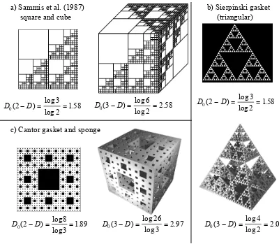
Generally, it is not possible to infer the fractal dimension of a 3-D fracture network from a

2-D network or from planar section through a 3-2-D network. This problem is illustrated in figure

16, where a) shows a modified Sierpinski gasket proposed by Sammis (1987) to model

fragmented rock found in fault zones. Here, the adding of one embedding dimension simply

increases the fractal capacity dimension (D0) by one. However, in the general case, D0

(3-D)=D0(2-D) +1 is only true if D0(2-D) is the spatial average of all possible sections. For

example, if the fractal dimension of a Sierpinski Triangle is measured in a 2-D projection, then

D0(2-D)=1.58, but the entire 3-D pyramid gives D0(3-D)=2.0. In figure 16a, all 2-D sections

parallel to a face have the same fractal dimension. In figures 16b and 16c, the 2-D fractal

dimension varies with the orientation of the section.

Interpreting this observation with respect to a random (natural) fractal suggests that simple

up-scaling of fractal dimension with embedding dimension only holds if the structure is

homogeneous, i.e. where all 2-D sections have the same fractal dimension.

As a result, the mapping of fractures and faults in 2-D sections (e.g. outcrop mapping and in

D₀ 2 D 3

2 1 58

( ) log

log .

- = = D0 3 D

6 2 2 58

( ) log

log .

- = = D0 2 D

3 2 1 58

( ) log

log .

- = =

D₀ 3 D 4

2 2 0

( ) log

log .

- = =

D0 2 D

8 3 189

( ) log

log .

- = = D0 3 D

26 3 2 97

( ) log

log .

- = =

a) Sammis et al. (1987) square and cube

b) Sierpinski gasket (triangular)

c) Cantor gasket and sponge

Figure 16: a) Two- and three-dimensional illustrations of the idealised fractal structure (modified Sierpinski gasket) for fault zones proposed by Sammis et al. (1987). Note that the 3-D version shows a fractal capacity

2.3.6 The problem of multi-fractals and lower/upper cut-off length scales

It is clear that the structure of many materials in nature, especially if they are fractured, is not

the result of just one process. Instead, a sequence of several processes will act to shape,

modify and characterise the properties of any rock mass. Examples include several phases of

tectonic deformation, mineral dissolution and precipitation, diagenesis and sedimentary

reworking etc. It will be shown in a later section that the fractal properties of fractured rock

are related to the governing fracturing mechanism. Hence it becomes clear that several fractal

structures might be superimposed in natural rocks. This leads to the problem of multi-fractal

structures.

In the strict mathematical sense, multi-fractal structures are defined by their local fractal dimension, which might not be a constant (Takayasu, 1989). Space-varying fractal dimensions

are related to a cascading frequency spectrum and will not be considered further in this study.

Other researchers have used the term “multi-fractal” for log-log plots that can be approximated

by more than one straight line. Then the structure has a constant fractal dimension only over a

certain length range. This leads to the problem of cut-off length scales. As described in section

2.3.1 , the fractal dimension is defined over an infinite number of length scales. In nature,

however, this is only approximated: There are physical limits on the smallest and the largest

scale over which structures can be self-similar. For example, Garrison et al. (1993a,b) found

that the smallest pore-size generation observed in thin-sections do not seem to contribute very

much to measured core-plug air permeabilities and a better fitting fractal exponent was

obtained when the first pore-size generation was omitted.

Even though Karasaki et al. (1988) found that very small fractures might not be important for

modelling flow in fractured media, and might be approximated by an equivalent porous block

approach, Acuna and Yortsos (1995) report that numerical simulation of flow through fractal

networks is only similar to the analytical solution if the object is fractal over a large enough

range of scales. Otherwise, finite size and storage effects may dominate the pressure response

and make the identification of the structure difficult. This emphasises the importance of

considering finite length scales that are either imposed my computational constraints in the

2.4 Review of fractal structures in hydrogeology

2.4.1 Introduction

Fractal dimension measurements have been reported by many researchers in the field of earth

sciences. This section aims to demonstrate that fractal theory is not only a good method to

describe a power-law behaviour between different parameters (as a mathematical model

approximation), but also that fractal structures seem to intrinsically govern many of the

processes that are important in hydrogeology. Applications of fractal measurements in the

earth sciences can be categorised into the following fields:

• testing whether some feature shows fractal scaling

• characterisation of surface geometry to determine some internal property

• use of fractal geometry to study formation and degradation processes

• use of fractal slopes to determine multiple processes and the scales over which they are

dominant

• use of fractal geometry as a tool for interpolation and extrapolation

• use of fractal geometry to derive empirical equations to estimate parameters that are

difficult to measure.

A good review of fractal applications in the earth sciences was given by Takayasu (1989) and

Cox and Wang (1993). Table 2, modified after Cox and Wang (1993), shows applications and

methods used. This review shall focus on applications of fractal measures on properties that

are of direct interest for hydrogeological investigations and may directly determine apparent

diffusivity and connectivity, such as

• pore geometry (aggregate, particle and void size distribution)

• fracture surfaces (roughness)

• fault traces (surface mapping and borehole intersections)

• fracture networks

Method Reference Application E - D Divider Norton et al., 1989 Granite mountain profile .15 to .28

Divider Snow, 1989 Stream channels .04 to .38

Divider Aviles et al., 1987 San Andreas Fault trace .0008 to .0191

Divider Brown, 1987 Rock fracture surface .50

Divider Carr, 1989 Rock fracture surface .0000 to .0315

Divider Miller et al., 1990 Rock fracture surface .058 to .261

Divider Underwood et al., 1986 Steel fracture .351 to .512

Divider Akbarieh et al., 1989 Erosion of Ca-oxal, crystals .025 to .106

Divider Kaye, 1986 Carbon particles .32

Divider Kaye, 1986 unpolished Cu surface .47

Divider Kaye, 1986 polished Cu surface .00

Box Barton and Larsen, 1985 Rock fracture network .12 to .16

Box La Pointe, 1988 Rock fracture network .37 to .69

Box Miller et al., 1990 Rock fracture network .041 to .159

Box Hirata, 1989 Japan fault network .05 to .6

Box Okuba and Aki, 1987 San Andreas Fault trace .2 to .4

Box Sreenivasan et al., 1989 Turbulent flow interface .35

Box Langford et al., 1989 Epoxy fracture .35

Box Langford et al., 1989 MgO fracture .16

modified Box Garrison et al., 1993 carbonates and sandstone empirical eqn. K & E

Triangle Denley, 1990 Gold film surface .04 to .46

Slit-island Mecholsky and Mackin, 1988 Chert fracture .12 to .32

Slit-island Schlueter et al., 1991 Sandstone pores .31 to .40

Slit-island Schlueter et al., 1991 Limestone pores .20

Slit-island Huang et al., 1990 Steel fracture surface (lakes) .20 to .30

Slit-island Huang et al., 1990 Steel fracture surface (islands) .33 to .40

Slit-island Mandelbrot et al, 1984 Steel fracture surface .28

Slit-island Pande et al., 1987 Titanium fracture surface .32

Slit-island Langford et al., 1989 Epoxy fracture surface .32

Spectral Gilbert, 1988 Sierra Nevada topography -0.835 to .471

Spectral Brown and Scholz, 1985 Rock fracture .26 to .68

Spectral Carr, 1989 Rock fracture -0.880 to .467

Spectral Miller et al., 1990 Rock fracture .124 to .383

Spectral Mandelbrot et al., 1984 Steel fracture .26

Spectral Langford et al., 1989 Photon emiss. from epoxy fract. .45

Variogram Burrough, 1983 Soil pH variation .6 to .8

Variogram Burrough, 1983 Soil Na variation .7 to .9

Variogram Burrough, 1983 Soil elec. resist. variation .4 to .6

Variogram Armstrong, 1986 Soil microtopography .64 to .90

Distribution Curl, 1986 Cave length, volume .4, .8

Distribution Krohn, 1988a Sandstone pores .49 to .89

Distribution Katz and Thompson, 1985 Sandstone pores .57 to .87

Distribution Krohn, 1988b Carbonate and shale pores .27 to .75

Distribution Avnir et al., 1985 Carbonate particles .01 to .97

Distribution Avnir et al., 1985 Soil particles .43 to .99

Table 2: Measured fractal dimension for different geological applications. The right column denotes the difference between the Euclidean embedding dimension E and the fractal dimension D as determined by the method indicated in the left column. Applications relevant to Hydrogeology are highlighted.

2.4.2 Pore geometry

It is well known from Poiseuille’s law that the rate at which a fluid can travel through a porous

medium is controlled by the flow paths that are open to flow. This flow path is a subset of

the overall geometry of the pore system. Garrison et al. (1992, 1993) showed that the

apparent surface fractal dimension DS, obtained from the pore diameter vs. number

distribution, exhibits a wide range of values for any particular rock type. This distribution

contains information about lacunarity and multiple fractal processes. They showed that there

is an empirical relationship between measured core plug air permeability, shape factor and

pore similarity fractal dimension DS, which is valid for several different reservoir rock types.

Figure 17 shows that only the fractal similarity dimension DS and the shape factor Sa are

needed to account for all of the variability in measured core plug permeability. This is

obviously of great use in situations where no core can be taken and only rock chippings or

fragments are available because only a small thin section of the rock is needed to measure the

necessary parameters.

log[ k(air) measured]

D_S (simil. dimension)

S_a (shape factor)

Norphlet Sandstone Spraberry Sandstone Arun Limestone San Andres Dolomite

Figure 17: A 3-D plot, in log(k)-DS-Sa space, of measured core plug air

permeability vs. apparent similarity dimension DS and area shape factor

Sa for the pores of the controlling process in samples of various

Researchers that have used fractal dimensions to classify pore geometries include Katz and

Thompson (1985), Krohn and Thompson (1986) and others (see review by Thompson,

1991). The method used usually is to analyse the fractal geometry of the pore structure of

sedimentary rocks by imaging impregnated thin sections and counting the number of pores for

different diameters. Avnir et al. (1985) re-analysed existing particle distribution data of

particle aggregates of different origin (carbonates, quartz-, rock- and soil particles). They

found distinct fractal dimensions for carbonate rocks of different origin.

2.4.3 Fracture surfaces

Fracture surfaces have been the subject of intense study in connection with rock

characterisation for subsurface nuclear waste repositories. This interest was motivated by the

observation that flow is often observed to be channelled along fracture planes rather than

flowing across the whole fracture plane. The amount of this channelling is controlled by the

roughness of fracture surfaces.

Both, field and laboratory rock fractures have been analysed by several researchers. In the

field, natural fractures that formed after the disruption of mineral grains, rock fragmentation

and matrix filling are subjected to further movement along the fault and filling of the fracture

by fluid flow interaction. This complicates the interpretation of natural fracture surface

topography.

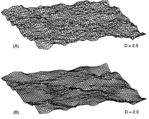
Brown and Scholz (1985) measured parallel sets of profiles across both laboratory and

field-scale rock surfaces. They included different fracture types such as bedding planes, fault planes

and glacial surfaces. The measured fractal dimension was then used to generate rough surfaces

(figure 18) and to evaluate fluid flow on fractures composed of rough surfaces. Fluid flow was

then simulated between these surfaces. Brown and Scholz concluded that fractal dimension

was constant only over limited ranges of spatial frequency and also that the fractal description

of fractal surfaces offers an advantage over topographic measurements because other

roughness measures are not constant over different scales. However, it was also found that

variations of fractal dimension produce only second order effects on the fluid flow.

Carr (1989) evaluated the effect of using different fractal dimension techniques (spectral

found that the divider method is most suitable to correlate the fractal dimension of the Yucca

Mountain fracture surfaces with the roughness coefficient.

Miller (1990), on the other hand, found that the correlation between fractal dimension and

roughness of fracture surfaces is poor and that the main use of fractal dimension

characterisation is the ability to support simulations and visualisations rather than as a means

to uniquely describe fracture roughness.

Figure 18: Examples of fractal surfaces used in the simulations. Both surfaces have the same root-mean-square height. Both were generated with the same set of random numbers but with different fractal dimensions: A) 2.5 and B) 2.0.

(After Brown, 1989)

2.4.4 Mapping of fault traces and lineaments

The mapping of fault traces and lineaments is probably the field with the most direct

applicability to fractured rock hydrogeology. Many publications have reported the

measurement of fractal dimensions obtained from fault traces at the surface and in boreholes.

Scholz and Aviles (1986) digitised fault traces from the San Andreas Fault and found a

spectral fractal dimension ranging from 1.1 to 1.5. Okuba and Aki (1987) used the box

counting method on traces from the San Andreas area, trying to relate strain release to the

obtained in this way were between 1.12 and 1.43. Aviles (1987) used the divider method and

obtained a fractal dimension close to one.

The analysis of fault traces has also been extended to networks of branching fracture traces.

Hirata (1989) reports fractal analyses using the box counting method on fault systems in

Japan. One aim was to determine whether the structure of the fault system was self-similar.

The fractal dimensions obtained were between 1.05 and 1.60, with high values observed at the

centre of the structures, decreasing away from the centre of the Japan Arc.

Barton and Larsen (1985) and La Pointe (1988) measured the fractal dimensions of fracture

networks in rock pavements for areas ranging from 200 to 300m2_{. Barton and Larsen found}

that for Miocene ash-flow tuff pavements at the Yucca Mountain Range fractal dimensions

range from 1.10 to 1.18. The fracture trace length followed a log normal distribution. A

sub-analysis of the same data showed that, even though the fracture networks appeared visually

different, the fractal dimension of different networks was similar (1.12, 1.14 and 1.16).

La Pointe (1988) developed an index of fracture density based upon fractal dimension for two

dimensional visualisations of fractures. He used two approaches, in one of them the number of

fractures per unit area of rock is counted for each different grid spacing. The second approach

counts the number of blocks bounded by fractures in each grid. It was found that fracture

density, as determined by either method, was fractal and scale invariant. The study also

concluded that the block size distributions may be controlled significantly by the fractal

dimension of the geology.

2.4.5 Fractal relationship between fault number, lengths and widths

Watanabe and Takahashi (1995) have given a very good example of the usefulness of the

fractal characterisation of fault traces. They researched the properties of fractured rocks with

respect to their use as geothermal reservoirs. Instead of using the box counting method, which

gives a measure for the spatial distribution of fractures, they use a power-law relationship

between observed fracture length r and the number of fractures N whose length is equal to or

larger than this length. This can be expressed by the equation N =Cr-D, where C is a fracture

density parameter. This study also compared fractal networks simulated by using the

to obtain flow is significantly lower than that of percolation models. This study demonstrated

that it is possible to characterise a subsurface fracture network with a few parameters obtained

from borehole data.

Main, Meredith et al. (1990) reported a value for the fractal dimension measured in this way

of 1.3. This relationship is related to the observation that earthquake fault length, slip (and

therefore magnitude) and frequency also scale as a power-law (Scholz and Cowie, 1990).

Hence, this is strong (albeit circumstantial) evidence that the fractal relationship observed

between different fault parameters are caused by the underlying fracturing mechanisms.

A similar relationship has been reported by Thomas and Blin-Lacroix (1989) for fractures with

width w and the number of fractures whose widths are equal to or larger than w. Since fracture

aperture and length directly determine the hydraulic conductivity of a given fracture, a

fractional flow dimension can also be expected.

2.4.6 Fractal distribution of three-dimensional fracture networks

Robertson and Sammis (1995) have reported a novel approach to the fractal analysis of

fracture networks. Although many studies that were reviewed above have demonstrated that

faults and fractures are self-similar over a large range of scales in two dimensions, none have

attempted to extend a fractal analysis to three dimensions. It is, of course, difficult to obtain a

good representation of the orientation of fractures in three dimensions with conventional

methods. Robertson and Sammis, however, used earthquake hypocentral locations in central

and southern California to “illuminate” three-dimensional fault structures, for which the three

dimensional capacity dimension D0(3-D) was obtained. Aftershocks and background seismic

events were found to show a fractal pattern, asymptotically approaching a constant dimension

value for a large number of events. D0(3-D) dimensions reported for three different earthquake

zones were 1.92±0.02, 1.82 and 1.79. As has been shown in section 2.3.5, it is not always

possible to infer the fractal capacity dimension of a 3-D fracture network from a 2-D planar

section. Nevertheless, the values reported here are not much higher than the 2-D values

reported in the section above, even though they could be expected to be from the example of

homogeneous fractal structures, where adding one embedding dimension also increases the

earthquakes only occur on the “percolation ba