Abstract—An algorithm is presented for in situ omnidirectional vision-based bee counting on landing pads of Langstroth beehives. The concept of the 1D Haar Wavelet Spike is developed. The spikes are detected in the 1D Haar Wavelet Transforms of image rows. The algorithm is implemented in Python 2.7.9 with OpenCV 3. The performance of the algorithm was tested in situ on a Raspberry Pi 3 Model B computer with an ARMv8 processor and 1GB RAM with a sample of 382 720 x 480 PNG images. The images were captured by a Raspberry Pi Camera Board v2 connected to a multi-sensor electronic beehive monitoring device. The algorithmic bee counts approached a human beekeeper’s counts within a margin of 5 bees on 63% of the images, within a margin of 10 bees on 94% of the images, and within a margin of 15 bees on 99% of the images.
Index Terms—computer vision, discrete wavelet transform, biosensors, electronic beehive monitoring, sustainable computing
I. INTRODUCTION
rofessional and amateur beekeepers use visual estimates of forager traffic levels to evaluate bee colonies’ health. Higher levels of forager traffic may indicate onsets of swarms or colony robbing activities; lower levels of forager traffic may indicate mite infestations, failing queens, or chemical poisonings [1, 2].
Advances in electronic sensors have made it feasible to transform apiaries into sensor networks that collect multi-sensor data in situ to estimate bee colonies’ health [3]. Electronic beehive monitoring (EBM) can help researchers and practitioners collect data on colony behavior and phenology without invasive beehive inspections [4].
In this paper, an in situ computer vision (CV) algorithm is presented for omnidirectional bee counting on landing pads of Langstorth beehives [5] used by many U.S. apiarists [6]. The algorithm is omnidirectional, because it does not distinguish between incoming and outgoing bee traffic. Bee counts can be used as forager traffic level estimates.
The algorithm has been developed with open source software tools and tested on a hardware device assembled with off-the-shelf hardware components. A fundamental objective of this project is to create a suite of replicable hardware and software tools for citizen scientists to build their own EBM devices (EBMDs) and to promote the grassroots development of EBM cyberinfrastructures [7].
Manuscript received December 5, 2016; revised December 24, 2016. Vladimir A. Kulyukin is with the Department of Computer Science of Utah State University, Logan, UT 84322 USA (phone: 434-797-2451; fax: 435-791-3265; e-mail: [email protected]).
The remainder of this paper is organized as follows. In Section II, related work is reviewed. In Section III, the hardware and software details of BeePi© [8], a multi-sensor solar-powered EBMD, are presented. In Section IV, the concept of a 1D Haar Wavelet Spike (1D HWS) is formally developed. Section V describes the proposed algorithm. In Section VI, the algorithm performance is analyzed. In Section VII, conclusions are drawn.
II. RELATED WORK
EBM has been evolving for over half a century. In the 1950’s, Woods placed a microphone in a beehive and subsequently built Apidictor, an audio beehive monitoring tool [4]. Bencsik [9] equipped several hives with accelerometers and observed increasing amplitudes a few days before swarming, with a sharp change at the point of swarming. Evans [10] developed Arnia, a beehive monitoring system that uses weight, temperature, humidity, and sound. The system breaks down hive sounds into flight buzzing, fanning, and ventilating and sends digital alerts to beekeepers.
S. Ferrari et al. [11] assembled a system for monitoring swarm sounds in beehives. The system consisted of a microphone, a temperature sensor, and a humidity sensor placed in a beehive and connected via underground cables to a computer in a nearby barn. Rangel and Seeley [12] investigated signals of honeybee swarms. Five custom designed observation hives were sealed with glass covers. The captured video and audio data were monitored daily by human observers. The researchers found that approximately one hour before swarm exodus, the production of piping signals gradually increased and ultimately peaked at the start of the swarm departure.
Meikle and Holst [13] placed four beehives on precision electronic scales linked to data loggers to record weight for over sixteen months. The researchers investigated the effect of swarming on daily data and reported that empty beehives had detectable daily weight changes due to moisture level changes in the wood. Bromenshenk et al. [14] developed electronic SmartHive© devices equipped with electronic scales, infrared bee counters, temperature and humidity sensors, digital weather stations, and wireless communication lines for Internet-based remote monitoring.
The investigation in this paper continues our research on CV algorithms for omnidirectional bee counting [15]. Two algorithms have been previously proposed [16]. Unlike the algorithm in this paper, the previous algorithms were not in situ and had lower bee counting accuracies (see Sections VI and VII for comparative performance details).
In Situ Omnidirectional Vision-Based Bee
Counting Using 1D Haar Wavelet Spikes
Vladimir A. Kulyukin
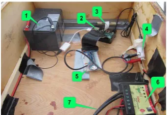
Fig. 1. Main hardware components of BeePi: 1) battery; 2) RPi; 3) RPi camera board; 4) car charger; 5) breadboard; 6) solar charge
controller; 7) solar panel wires.
III. MULTI-SENSOR EBM
CV is one of the sensors in BeePi, a multi-sensor, solar-powered EBMD. Each BeePi consists of a Raspberry Pi (RPi) computer, a camera, a solar panel, a temperature sensor, a battery, a hardware clock, and a solar charge controller. The current version of BeePi is 1.1. The main BeePi hardware components are shown in Fig. 1 and include a RPi 3 Model B with 1GB RAM (Model B+ 512MB RAM was used in BeePi 1.0), an RPi T-Cobbler, a full-size breadboard for sensor integration, a waterproof DS18B20 digital temperature sensor, an RPi Camera Board (CB), and a USB microphone hub.
Unlike BeePi 1.0, the previous version of BeePi, BeePi 1.1 uses the RPi CB v2 instead of v1. In BeePi 1.0, the camera of the RPi CB was protected only with a plastic cover, which was found to provide inadequate protection against rain, snow, and strong wind after five weeks of field deployment in Northern Utah in 2014-2015 [15, 16]. In BeePi 1.1, the camera is not only placed under a plastic cover, but also is attached to a wooden plank for improved balance; the plank is attached with screws and metallic brackets to the super with the BeePi hardware, as shown in Fig. 2. The camera is protected from the elements by a wooden protection box opened at the bottom and attached to a hive lid with screws and metallic brackets (see Fig. 3a). When the lid is placed on the super with the BeePi hardware (see Fig 3b), the box protects the camera (and all other sensors on the plank) against the elements from above and the four sides.
For solar harvesting, we continue to use Renogy 50 watts 12 Volts monocrystalline solar panels, Renogy 10 Amp PWM solar charge controllers, Renogy 10ft 10AWG solar adaptor kits, and the UPG 12V 12Ah F2 sealed lead acid AGM deep-cycle rechargeable batteries. The solar panels are placed either to the right or left of a beehive or behind a beehive on the ground.
It takes approximately 25 minutes to wire a BeePi EBMD for deployment. Fig. 4 shows the author wiring two EBMDs for deployment in Northern Utah in early May 2016. Data collection is done on the RPi. The collected data are saved on a 32G sdcard inserted into the RPi. Data collection software is written in Python 2.7.9. When the system starts, three data collection threads are spawned. The first thread collects temperature readings every 5 minutes and saves them into a text file. The second thread collects 30-second wav recordings every 5 minutes. The third thread saves PNG
pictures of the beehive’s landing pad every 5 minutes. A cronjob monitors the threads and restarts them after hardware failures.
Fig. 2. Camera (1) under plastic cover attached to wooden plank (2); plank is attached with metallic brackets (3) to box with BeePi
hardware; camera looks down on hive’s landing pad (4).
(a) Protection box from inside (1); box is attached to migratory lid (2).
(b) Hive lid (1) with protection box (2) on hive; solar panel (3) on ground.
[image:2.595.317.537.98.188.2]Fig. 3. RPi camera board protection against elements.
Fig. 4. Wiring BeePi 1.1 hardware for deployment.
IV. 1DHAAR WAVELET SPIKES
In the 1D Haar Wavelet Transform (1D HWT), a signal is a vector in
R
n,
n
2
k,
k
N
.
Following the formalization in [17], letW
a k be a2
k
2
kmatrix for computing k scales of the 1D HWT. This matrix can be effectively computed from the n canonical base vectors ofR
n.
If
0,..., 2 1
x x k
x is a signal in
R
n, theny
is the k-scale1D HWT of
x
is defined in (1).
x
y
W
ak
T
(1)Then
1
1 2 1 0 1 1 1 0 0 0 0
0 , , , ,..., ,..., 1
k k
T
k
c c c c c a
y (2)
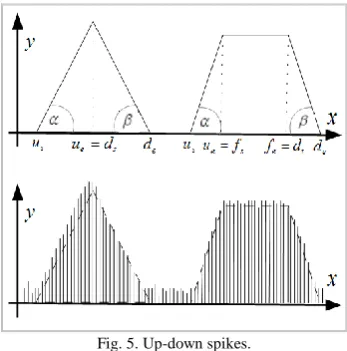
[image:2.595.318.537.224.373.2] [image:2.595.331.521.380.488.2]Fig. 5. Up-down spikes.
HWTs are used to detect significant changes in signal values [19]. In this paper, it is proposed that some changes can be characterized as signal spikes. Specifically, four types of spikes are proposed: up-down triangle, up-down trapezoid, down-up triangle, and down-up trapezoid. The difference between up-down and down-up spikes is the relative positions of the climb and decline segments. In trapezoid spikes, flat segments are always in between the climb and decline segments. Fig. 5 shows up-down triangle and trapezoid spikes; Fig. 6 shows down-up triangle and down-up trapezoid spikes. In both figures, the lower graphs represent possible values of the corresponding Haar wavelets at a given scale k. Formally, a spike is a nine element tuple whose elements are real numbers given in (3).
us,ue,,fs,fe,,ds,de,
(3)The first two elements,
u
sandu
e, are the abscissae of the beginning and end of the spike’s climb segment, respectively, when the wavelet coefficients of the 1D HWT increase. Ifcu
s k andcu
e k are the k-th scale wavelet coefficient ordinates atu
sandu
e,
respectively, then the climb segment of the spike is measured by the angle
1
,
.
tan
1 skk e s
e
u
cu
cu
u
The decline segment of thespike is characterized by
d
s,
d
e,
and
,
wheres
d
andd
eare the abscissae of the beginning and end of the spike’s decline segment, respectively, when the wavelet coefficients decrease. If ks
cd and k e
cd are the k-th scale wavelet coefficient ordinates at
d
sandd
e,
respectively, then the decline segment of the spike is measured by theangle
k
s k e s
e d cd cd
d
, 1 tan 1
.In trapezoid up-down or down-up spikes, the flat segment is characterized by
f
s,
f
e,
and
,
wheref
sandf
eare the abscissae of the beginning and end of the spike’s flat segment, respectively, over which the wavelet coefficients either remain at the same ordinate or have minor ordinate fluctuations. Ifcf
s k andcd
e k are the k-th scale waveletcoefficients corresponding to
f
sandf
e,
respectively, the spike’s flatness angle is
k
s k e s
e f cf cf
f
, tan 1
.
The absolute values of
are close to 0. V. BEE COUNTING ALGORITHMGiven an image, spikes can be computed for each row. When spikes are computed for row
r
, the column indices of the actual pixels covered by each spike at scale j are computed by the formula in (4), where s and e are the positions of the starting and ending wavelet coefficients in the 1D HWT at scale j, respectively. For up-down spikess
u
s
andd
d
e, whereas, for down-up spikes,s
d
s
ande
u
e.
j,s,e
i|2 si2
e11
[image:3.595.312.549.131.505.2]p j j (4)
Fig. 6. Down-up spikes.
Let n be the number of rows in an image and let
U
rbe the set of up-down spikes in rowr
,
0rn1. The set of pixel columns in rowr
covered by the up-down spikes inr
is given in (5), where j is a scale ands
zande
zare the beginning and end positions of an up-down spikez
in row,
r
respectively.
r
U z
z z r
j
U p j s e
Z
, ,
, (5)
Let
D
rbe the set of down-up spikes in rowr
,
. 1
0rn The set of pixel columns in
r
covered by the down-up spikes is given in (6), where j is a given scale ands
zande
zare the beginning and end positions of a down-up spikez
in rowr
,
respectively.
r
D z
z z r
j
D p j s e
Z
, ,
The number of unique column pixels covered by the up-down and up-down-up spikes in row
r
is given in (7). The formula in (8) gives the actual number of pixels covered by the up-down and down-up spikes in an imageI
with n rows.
r
j U r
j D r
j U r
j D r
j D r
j U r
j Z Z Z Z Z Z
Z , , , , , , (7)
1
0
n
r r j
j I Z
X (8)
For example, consider three 16 x 16 images in Fig. 7. Suppose it is required to separate bee pixels from non-bee pixels in the original bee image on the left. The bee pixels are those covered by up-down and down-up spikes in each row. The middle image in Fig. 7 shows the only up-down spike detected in row 8 after a single scale of the 1D HWT. The right image in Fig. 7 shows the only down-up spike detected in row 7. Both spikes are triangle ones.
Fig. 7. Bee image (left); up-down spike in row 8; down-up spike in row 8; up-segments are red; down-segments are blue.
The up-down spike, shown in the middle image in Fig. 7, is defined in (9), where, per notation in equation (3),
,
4
/
/3,
0
,
and the rest of the values are as follows:u
s
3
,u
e
4
,d
s
5
, andd
e
5
. The value of
1
forf
sandf
e indicates that the spike does not have a flat segment.
3,4,,1,1,,5,5,
(9)The down-up spike (see the right image in Fig. 7) is
defined in (10). Since this is a down-up spike, the beginning and end positions of the climb segment, i.e., 3 and 4, follow the beginning and end positions of the decline segment, i.e., 1 and 2, and the absolute values of
,
,and
are approximately the same as in the up-down spike in (9).
3,4,,1,1,,1,2,
(10)Using (5), the pixel columns of the up-down spike in (9) are given in (11).
1,3,5
|6 11
81
, p i i
ZU (11)
Using (6), the pixel columns of the down-up spike in (10) are given in (12).
1,1,4
|2 9
8 1
, p i i
ZD (12)
Using (7), the set of pixel columns covered by the two
spikes in row 8 in Fig. 7 (middle and right) is given in (13).
10,11
2,3,4,5
6,7,8,9
2,3,4,5,6,7,8,9,10,11
8 1 , 8
1 , 8
1 , 8
1 , 8
1 , 8
1 , 8 1
ZU ZD ZD ZU ZD ZU
Z
(13)
Given the number of scales
j
1
, the number of bee pixels in the left image in Fig. 7 is given in (14), where I is the left image in Fig. 7.
4415
0 1
1
r
r
Z I
X (14)
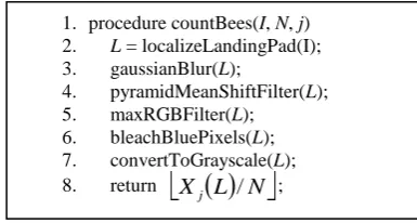
[image:4.595.51.283.295.358.2] [image:4.595.331.524.314.417.2]The pseudocode of the bee counting algorithm is given in Fig. 8. The algorithm takes an image I (e.g. the upper image in Fig. 9), the normalizer N, and the number of scales j of the 1D HWT. The algorithm also takes the thresholds for the angles of up-down, flat, and down-up spikes, i.e., α, γ, β, omitted for simplicity. In the current implementation, α = β = 60° and γ = 5°.
Fig. 8. Algorithm’s pseudocode.
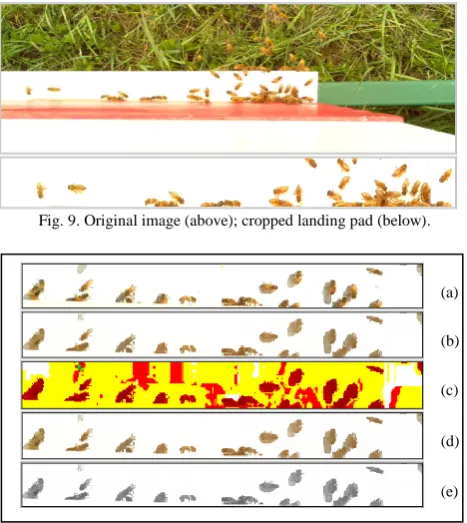
In line 2 of Fig. 8, the landing pad is detected and cropped from the original image. In Fig. 9, the lower image shows the landing pad cropped from the upper image. The landing pad localization algorithm is described in [15, 16].
In Fig. 10, all stages of image pre-processing, defined in lines 2 – 7 in Fig. 8, are shown beginning from the cropped landing pad region (Fig. 10a). The image in Fig. 10b is the result of the Gaussian blur of the image in Fig. 10a with a 7 x 7 kernel followed by the pyramid mean shift filter. The image in Fig. 10c shows the result of applying the max RGB filter to the image in Fig. 10b. The image in Fig. 10d shows the image where all blue pixels in Fig. 10c are set to white, which eliminates some shades that turn out as blue after the application of the max RGB filter. This bleached image in Fig. 10d is converted into grayscale, as shown in Fig. 10e.
In line 8 of Fig. 8, all pixels covered by up-down and down-up spikes in all rows are counted and the total count is normalized. The total count of bee pixels is normalized by
N. In the current implementation, N=60 since the average number of pixels per bee is 60. The total number of bee pixels detected by spikes normalized by the average number of pixels per bee gives an integer approximation to the number of bees on the pad.
VI. EXPERIMENTS
The algorithm’s accuracy was evaluated on a sample of three-hundred eighty two images captured by a BeePi EBMD deployed in Northern Utah. The images on which the
1. procedure countBees(I, N, j) 2. L = localizeLandingPad(I); 3. gaussianBlur(L);
4. pyramidMeanShiftFilter(L); 5. maxRGBFilter(L);
proposed algorithm was evaluated were captured in September 2016 when it is vital for beekeepers to keep abreast of colonies’ health as they prepare them for winter. In each image, the landing pad was localized and automatically cropped by the landing pad localization algorithm described in [15, 16]. A human beekeeper manually counted the bees in each image with a cropped pad. This beekeeper’s bee counts were taken as the ground truth. The algorithm was run on the same images and the number of bees detected in each image was recorded. Table I gives several lines from a file that contains the human and computer counts of bees for each image.
Fig. 9. Original image (above); cropped landing pad (below).
Fig. 10. Original image (a); blurred and mean shifted (b); max RGB filtered (c); bleached (d); grayscaled (e).
[image:5.595.309.540.227.354.2]Table II gives the accuracy of the computer algorithm compared with the ground truth. The first column, Error Margin, gives the allowed margin of error between the human and computer counts for each image. Images where the counts differed by more than the set margin were classified as inaccurate whereas images where the counts were within the allowed margin of error were classified as accurate.
TABLE I
Human vs computer counts of bees in images. Image Name Human Counts Computer Counts
2016-09-20_11-24-40.png 31 21
2016-09-21_18-14-43.png 30 33
2016-09-20_12-34-40.png 11 8
2016-09-21_07-54-42.png 1 1
The second column, Accuracy, in Table II gives the percentage of accurate images. Thus, for the margin of error equal to 5, 63% of the images were classified as accurate. When the margin of error is 10, 94% percent of the images were classified as accurate. When the margin of error is 15, 99% of the images were classified as accurate. The results in Table II suggest that the proposed algorithm is reasonably accurate in approximating human bee counts on pads.
Further analysis revealed that all errors, i.e., images where algorithmic counts differed from human counts by more than a given error margin were either excessively bright or had many shades. In Fig. 11, two sample images are shown on which the human and computer counts differed by more than 10 bees. Both images were taken by an EBMD mounted on a hive facing south. The upper image has a luminosity (a total amount of energy radiated by an object) above 253. On bright images, taken between 12:00 and 1:00pm, when the sun was directly above the hive, the algorithm undercounted. Specifically, in the upper image in Fig. 11, the human beekeeper counted 12 bees whereas the algorithm found only 1 bee.
Table II Error margin vs accuracy. Error Margin Accuracy (%)
5 63
10 94
15 99
Fig. 11. Two sample images on which bee counts differ by more than 10.
The lower image in Fig. 11 shows an image, taken between 4:00 and 6:00pm, when the sun was west of the hive. While the luminosity of such images is lower (the luminosity of the lower image in Fig. 11 is 206), there are noticeable shades to the east of some bees. Since some of these shades were not removed by the bleaching operation, the detected spikes included some shade pixels, which caused higher bee counts. Specifically, in the lower image of Fig. 11, the human beekeeper counted 33 bees whereas the algorithm found 65 bees.
Since the primary objective of the proposed algorithm is to keep abreast of the forager traffic levels and their changes over a period of time, the exact bee counts are less important than reliable, albeit approximate, indicators of traffic volumes. For example, it is insignificant, when forager traffic increases, to detect 60 bees when a human beekeeper detects 65 or 70, because both counts indicate an increase in forager traffic. Similarly, at smaller traffic levels, it is acceptable to detect 2 or 3 bees when a human beekeeper detects 5 or 7 bees, because both counts indicate a decline in forager traffic.
While algorithms’ accuracy is important, smaller RAM footprints should not be discounted, because they make feasible in situ execution on smaller computational devices with smaller power consumption footprints. Toward that end, the algorithm was implemented in Python 2.7.9 with OpenCV 3.0 on a RPi 3 Model B with an ARMv8 processor and 1GB of RAM. The real performance of the algorithm was evaluated with the Python timeit utility on the RPi. The timings, measured in seconds, for three different runs on all test images were 868.40, 869.76, and 863.07, with the mean time equal to 867.08. Thus, the algorithm, on average, took 2.27 seconds to process one image in situ. Since in deployed (a)
(b)
(c)
(d)
[image:5.595.50.290.612.677.2]BeePi EBMDs static frames of landing pads are taken every five minutes, the proposed algorithm, when executed on EBMDs, has sufficient time to process each picture and log timestamped bee counts.
VII. CONCLUSION
An algorithm was presented for in situ omnidirectional bee counting on Langstroth landing pads. The concept of the 1D Haar Wavelet Spike was developed. The algorithm was implemented in Python 2.7.9 with OpenCV 3.0 on a Raspberry Pi 3 Model B computer with an ARMv8 processor and 1GB of RAM.
The performance of the algorithm was tested in situ on the same computer with a sample of 382 720 x 420 PNG images. The algorithm took an average of 2.27 seconds per image. The algorithmic counts approached a human beekeeper’s counts within a margin of 5 bees on 63% of the images, within a margin of 10 bees on 94% of the images, and within a margin of 15 bees on 99% of the images. The algorithm is more accurate than our previous two algorithms for omnidirectional bee counting: the highest accuracy of the previous algorithms within a margin of 10 bees was 85.5% [8, 16]. Furthermore, unlike the algorithm presented in this paper, our previous two algorithms were not in situ in that they were implemented in JAVA with OpenCV 2 and evaluated on a 10GB RAM PC with Ubuntu 12.02 LTS.
Since the presented algorithm can operate on low voltage devices with smaller RAMs, it is more suitable for ecologically sustainable computing. Most approaches to EBM depend on the grid for power and on the cloud for data transmission (e.g., [9, 10, 11]). However, grid- and cloud-dependent EBM enlarges the electricity consumption and carbon footprints of cloud data centers which already account for two percent of overall U.S. electrical usage [20]. According to the Smart 2020 forecast by the Climate Group of the Global e-Sustainability Initiative [21], so far quite accurate, the global carbon footprint of cloud data centers is expected to grow, on average, 7% per annum between 2002 and 2020. In 2010, McAfee, a U.S. computer security company, reported that the electricity required to transmit the trillions of spam e-mails annually is equivalent to powering two million U.S. homes and generates the same amount of greenhouse gas emissions as that produced by three million cars [22]. Thus, there is a critical need to seek ecologically sustainable EBM solutions that use renewable power sources, capture data with software tools with smaller electricity consumption footprints, and minimally depend or do not depend at all on the cloud for data transmission or analysis. The proposed algorithm is a step on the long journey to ecologically sustainable EBM.
ACKNOWLEDGMENT
The author is grateful to Mr. Craig Huntzinger and Dr. Richard Mueller for letting him use their property in Northern Utah for longitudinal EBM tests. The author expresses his gratitude to Mr. Craig Huntzinger and Mr. Nathan Huntzinger for their help with inspecting monitored beehives and logging observations. All bee packages, bee hives, and beekeeping equipment used in this study were
personally funded by the author. REFERENCES
[1] J. Tautz. The Buzz about bees: biology of a superorganism. Heidelberg: Springer, 2008.
[2] D. Sammataro, A. Avitable. The Beekeeper’s handbook, 4th Edition.
Ithaca, NY: Cornell University Press, 2011.
[3] M. T. Sanford. "2nd international workshop on hive and bee monitoring," American Bee Journal, December 2014, pp. 1351-1353. [4] M.E.A. McNeil. “Electronic Beehive Monitoring,” American Bee
Journal, Aug. 2015, pp. 875 - 879.
[5] Rev. L. L. Langstroth. Langstroth on the hive and the honey bee: a bee keeper's manual. London: Dodo Press, 2008; orig. published in 1853.
[6] L. Crowder, H. Harrell. Top-bar beekeeping: organic practices for honeybee health. White River Junction, Vermont: Chelsea Green Publishing, 2012.
[7] http://honeybeenet.gsfc.nasa.gov/, NASA HoneyBeeNet Project. [8] V. Kulyukin and S. Reka. “Toward sustainable electronic beehive
monitoring: algorithms for omnidirectional bee counting from images and harmonic analysis of buzzing signals.” Engineering Letters, vol. 24, no. 3, pp. 317-327, Aug. 2016
[9] M. Bencsik, J. Bencsik, M. Baxter, A. Lucian, J. Romieu, M. Millet. “Identification of the honey bee swarming process by analyzing the time course of hive vibrations.” Computers and Electronics in Agriculture, vol. 76, pp. 44-50, 2011.
[10] W. Blomstedt. “Technology V: understanding the buzz with arnia.”
American Bee Journal, Oct. 2014, pp. 1101 - 1104.
[11] S. Ferrari, M. Silvab, M. Guarinoa, D. Berckmans. "Monitoring of swarming sounds in bee hives for early detection of the swarming period," Computers and Electronics in Agriculture. vol. 64, pp. 72 - 77, 2008.
[12] J. Rangel and T. D. Seeley. "The signals initiating the mass exodus of a honeybee swarm from its nest," Animal Behavior, vol. 76, pp. 1943 - 1952, 2008.
[13] W.G. Meikle and N. Holst. "Application of continuous monitoring of honey bee colonies," Apidologie, vol. 46, pp. 10-22, 2015.
[14] J. Bromenshenk, C.B. Henderson, R.A. Seccomb, P.M. Welch, S. E. Debnam, D. R. Firth. “Bees as biosensors: chemosensory ability, honey bee monitoring systems, and emergent sensor technologies derived from the pollinator syndrome.”Biosensors, 2015, vol. 5, pp. 678-711; doi:10.3390/bios5040678.
[15] V. Kulyukin, M. Putnam, S. Reka. “Digitizing buzzing signals into A440 piano note sequences and estimating forager traffic levels from Images in solar-powered, electronic beehive monitoring. Proc. of Intl. MultiConf. of Engineers and Computer Scientists (IMECS 2016):
Intl. Conf. on Computer Science, vol. I, pp. 82-87, Mar. 16-18, Kowloon, Hong Kong, IA ENG, ISBN: 978-988-19253-8-1. [16] V. Kulyukin, S. Reka. “A Computer vision algorithm for
omnidirectional bee counting at langstroth beehive entrances.” Proc. of Intl. Conf. on Image Processing, Computer Vision, and Pattern Recognition (IPCV'16), pp. 229-235, ISBN: 1-60132-442-1, CSREA Press. Las Vegas, NV, USA, Jul. 2016.
[17] A. Jensen, A. Cour-Harbo. Ripples in mathematics: the discrete wavelet transform. New York: Springer, 2001.
[18] Y. Nievergelt. Wavelets made easy. Boston: Birkhäser, 2001. [19] S. Mallat, W. Hwang. “Singularity detection and processing with
wavelets.” IEEE Trans. on Information Theory, vol. 38, no. 2, Mar. 1992, pp. 617-643.
[20] B. Walsh. “Your data is dirty: the carbon price of cloud computing.”
Time, Apr. 2, 2014.
[21] “Smart2020: Enabling the low carbon economy in the information age.” The Global e-Sustainability Initiative. Avail. at http://www.smart2020.org/_assets/files/02_smart2020Report.pdf. [22] M. Berners-Lee and D. Clark. “What’s the carbon footprint of …