A. Based on Canny method



Abstract— Obstacles detection systems are essential to achieve a higher level of safety on railways. Such systems should have the ability to contribute to the development of automated guided trains. Even though some laser equipments have been used to detect obstacles, short detection distance and low accuracy on curve zones make them not the best solution. In this paper, computer vision combined with prior knowledge is used to develop an innovative approach. A function to find the starting point of the rails is proposed. After that bottom-up adaptive windows are created to focus on the region of interest and ignore the background. The whole system can run in real time thanks to its linear complexity. It performs well in different conditions and it can work both on online and offline recorded video.

Index Terms— Transportation; Obstacles detection; Computer vision; Prior Knowledge, Video Forensic

I. INTRODUCTION

ITH the rapid development of economy, transportation became more and more important. Train is one of the safest means of transport, however several accidents still happened in recent years. In the development of automated guided trains, it is urgent to set up a system to help figuring out anomaly conditions in front of a running engine. Computer vision is always more advanced, but changing lighting conditions, background, and running speed make obstacles detection on railways a hard task. In this paper a system implemented in C++ and OpenCV is proposed. The system has the ability to tolerate changing environment and to find obstacles on or between the rails. It can therefore be a safety component for automated guided trains, but it can even represent a useful tool for the drivers of conventional trains. The paper is structured as follows. In section 2 some related works in subject of obstacles detection are presented. Section 3 describes our assumptions for the problem and the approach developed. Experimental results are shown in

Manuscript received January 8, 2017; revised January 18, 2017. Hui Wang. Author is with the Ulster University, Belfast, UK (e-mail: [email protected]).

Xiaoquan Zhang Author is Ulster University, Belfast, UK (e-mail: [email protected]).

Lorenzo Damiani Author is with University of Genoa ITALY (e-mail: [email protected]).

Pietro Giribone Author is with University of Genoa ITALY (e-mail: [email protected]).

Roberto Revetria Author (Corresponding author) is with University of Genoa ITALY (phone: 3339874234;e-mail:[email protected]).

Giacomo Ronchetti Author is with University of Genoa ITALY (e-mail: [email protected]).

section 4. Conclusions and future works are presented in section 5.

II. RELATED WORK

In the subject of obstacles detection on railways, there exist two basic ideas. The first one is based on the use of sensors, such as [1], [2], [3]. The other one is based on video processing. Sensors can find obstacles more easily but they cannot avoid the drawbacks of cost emitting devices, short detection distances and low accuracy on curve zones. So, even though there is not yet a perfect solution for the problem, video based methods may be a better choice. The current approaches can be mainly divided into two strategies: some of the ideas use Canny Operator, some others apply prior Knowledge. Using forensic video analysis is also possible to provide detailed reconstruction for accident dynamic and evaluate quantitatively the effects on human bodies as presented in [13] and [15].

A. Based on Canny method

Approaches based on Canny method [4] use Canny operator to extract edges from an image. The first step is to smooth the image by a Gaussian filter in order to decrease the influence of the noise. Then the gradient image is obtained using a Sobel operator. Finally non-maximum suppression is applied to sharpen the edges and two thresholds are used to detect the effective edges. [5] shows an adaptive way to find the thresholds for the Canny method. Its basic principle is to split the image’s pixels into two classes and to find the best threshold value through the maximum variance value between the two classes. However, it cannot get the edge of the rails because of the fickle background. [6] shows an obstacles detection method on railways based on Canny method. It uses a model train to imitate the real train and a small camera to get the video from the head of the train. Rails and sleepers show obvious geometric lines characteristics after Canny edge detection, obstacles undermine the integrity of these lines. Thus an obstacle on the condition that disconnected length of lines exceeds a certain threshold can be confirmed. The effect on Canny image is very clear, an obstacle can be detected in two aspects: one is through the number of consecutive pixels where the rails lines lie to determine the integrity of the rails, the other is by determining if the distance at both ends

of each sleeper is abnormal with regard to what expected. [7] finds the candidate obstacle areas based on the edge

detection. Then it trains a SVM to classify the candidate obstacle areas and to verify whether they represent a real

Video Analysis for Improving Transportation

Safety: Obstacles and Collision Detection

Applied to Railways and Roads

Hui Wang, Xiaoquan Zhang, Lorenzo Damiani, Pietro Giribone, Roberto Revetria, Giacomo Ronchetti

obstacle or not, using features such as dimension and colour information of these areas. Even though using Canny method is a good way to generate rails intuitively, it suffers the drawback of selecting effective thresholds and shadows may make the conditions even worse. Figure 1 shows the different results of two thresholds. The original image of a railway, the result of an adaptive threshold and the result of a low threshold are shown. We can figure out the importance and the difficulty of choosing a proper threshold.

Fig. 1. Result of different thresholds.

A. Based on Prior Knowledge

Prior knowledge for image analysis on railways is mainly based on two concepts, the first one is that rails are always in the picture and they meet at the top of the image, the second one that rails from bird’s-eye view are always parallel. [8] is based on the fact that the rails look like lines projecting from the bottom of the image to the horizon and they seem to converge in a far point. In the vicinity of the driver zone, the rails appearance is quite monotonous, while on the horizon it exists greater variability, especially in curve sections. To delimit a region of interest is the first task to start the search for obstacles and to decide if the way is free and can be safely travelled. In this case the rails, the area between them and the close outer area represent the zone of interest. One strategy for detecting the rails consists in extracting the lines in the image and selecting the most likely candidates to be the rails. They used the Hough transform to detect the rails in each frame and to start the delimitation of the region of interest to check for obstacles. [9] presented a comparison of various techniques for rails extraction. Then they introduced a new generic and robust approach. The algorithm uses edge detection and applies simple geometric constraints provided by the rail characteristics. [10] uses Canny method to get the rails. Then it gets the bird’s-eye view image by trapezoidal projection and it creates a region of interest moving from the bottom to the top of the image. In the ROI, a function grope_rails (R; ae; ge) is created to find the pair of lines with the maximum score. It restricts the angle ae and the gap ge to make it run in real time. However, there can be problems

when there are more than one pair of lines in the region of interest.

III. NOVEL APPROACH

After sufficient studies on previous works, we decided to develop an adaptable and less fine-tuned parameters method. We create a novel linear way to detect rails and to check for obstacles, based on four assumptions:

1. The gap between the rails at the initialization stage has to be constant.

2. The starting position of the rails cannot move saltatorial.

3. The pair of rails in the bird’s-eye view has to be parallel.

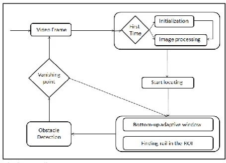
4. The pair of rails has to come to a vanishing point. The first two assumptions rectify the false conviction that the starting position has to be constant. The bird’s-eye view image helps to identify obstacles between the rails and the last assumption is the stop condition for the system. Figure 2 shows the system diagram designed according to the previous assumptions.

Fig. 2. System diagram.

The system collects video information from a camera mounted in front of the train and analyzes each frame. For each frame the methodology works as follows:

1. Pre-processing, it includes initialization and image processing.

2. Locating the start of the rails.

3. Creating bottom-up adaptive windows and finding the rails.

4. Checking for obstacles.

5. Next frame or back to the step 3.

B. Initialization

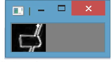
operator. We get the gradient value by using Euclidean distance.

Fig. 3. Raw frame and gradient image.

C. Locating the Start of the Rails

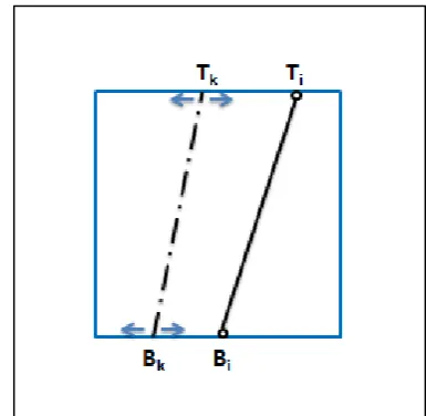
After we get the gradient image, we need to locate the start of the rails in order to create bottom-up windows and to check for obstacles. This method applies the assumption that the gap between the rails is constant and it does not move in a saltatorial way. The idea is shown from a geometrical point of view in figure 4. which case(s)

To make it a real time operating system, the algorithm has to be linear. In order to do so, we first create a pair of sliding windows. The gap between the windows is the gap between the rails and it is read from the configuration file. After that, we define a function f(x) such that:

Fig. 4. Locating the start of the rails.





ln 1 )

(

0 0

,

0 0

,

lp x g

g x

f

l

i h

j

j i gap x l

i h

j j i

x  _

  

 









   

  

gi,j is the gradient value at the pixel (i,j), lp and gap are the x-coordinate of the left rail and the gap between the rails respectively and they are recorded in the configuration file. This function calculates the sum of gradient values in the pair of sliding windows multiplied by a penalty factor. In order to ensure the penalty function has a relevant, but not decisive, impact on the windows position, we use reciprocal of natural logarithm of the distance between the x variable and the left position to be a penalty. In this way, when the position of the left window matches with the position recorded in the configuration file, that is supposed to be correct, the penalty function becomes irrelevant and the variable x is more likely to get a high score of f(x). On the other hand, a pair of windows is penalized if it has a position different from the expected one. We move the pair of sliding windows from the left to the right to get the maximum value of f(x) and consequently to find the position of the windows. We assume the length of the windows is L, and therefore the left rail should lie in the range [x; x + L] and the right one in the range [x + gap; x + gap + L]. This function allows to find the rail roughly. After we get windows, local maximization is applied to find a more accurate position of the rails. We get a line [Tk;Bk], where Tk is a point at the top and Bk is a point at the bottom edge of each window. Local maximization is to find the line with the maximal average gradient value that is supposed to be the rail. So we can get the local maximal line for each window [Ti;Bi], [T’i;B’i]. Bi and B’i are set to be the starting position of each rail.

Fig. 5. Local maximization.

Since we move the sliding windows horizontally, the time complexity of finding their position is O(w). w is the width of the image. After we get the pair of windows, finding the correct position of the rail in the window is O(L2), and since

D. Creating bottom-up windows

After finding out the starting position of the rails, adaptive bottom-up windows are created through an iterative process. It is desirable the windows to contain the same amount of information, so the top windows will be smaller than the bottom ones. The adaptive windows perform in two ways: size and position. Since we assume that the rail in the window is a line, the scale ratio between two adjacent windows is linear. The upper windows are generated through an iterative process and their size is defined by the following equations:

i i

i i

B B

T T L L

   

' ' '

i i

i i

B B

T T H H

   

' ' '

The rail is consistent and therefore the top point of the rail in a window is supposed to be the bottom point of the rail in the adjacent one. The position of the window is adaptive since the angle of the rail can change sharply in the small windows. The position of the window changes according to the top position of the rail in the lower window. As shown in figure 7 (a), if, for instance, the position Ti is on the right corner of the window, we claim the rail may be deflected sharply to the right. In such condition, the next window is created at the right corner in order to keep the rail inside. The same happens when Ti is on the left (c), obviously. When Ti is in the middle, the next window is centred on the previous one (b). The position of the adaptive windows is therefore strictly related to Ti and it responds well wherever a sharp deflection appears.

Fig. 6. Creating bottom-up windows.

After we fix the position of the next window, we apply local maximum idea to get the maximal average gradient line to be the rail. Subsequently the obstacle detection stage is worked. If there are no obstacles in the window, the next pair of top windows is generated. This process is iterated until the vanishing point is reached. The vanishing point is considered reached when the left window intersects with the right window, as shown in figure 8. The time complexity is still linear since, when we get the rail, the bottom point is already set as in the previous stage.

Fig. 7. Adaptability of the windows.

Fig. 8. Iteration of the process.

E Obstacles Detection

Every time a pair of bottom-up windows is created, the obstacle detection stage is worked. Three methods to check for obstacles on the railway are used.

1) Compare the angle generated by the lines detected between two adjacent windows. If the angle is sharper than a certain value, there might be an obstacle or the rail could be broken. The threshold value is looser for the windows further away because of the zoom rate. Figure 9 shows a gradient image where a brick lies on the left rail generating an anomalous angle between the lines detected by the system. In this case, the algorithm correctly assumes there is an obstacle obstructing the rail.

Fig. 9. Obstacle on the rail.

Here again the value becomes looser when the windows get higher in the image. If an obstacle is detected here, we check if most of the pixels do not come to an average value. If it is true, a shadow may hide the light.

3) In order to check for obstacles in the middle of the railway, trapezoidal projection to get the bird’s-eye view image is used. We get the projection matrix by trapezoidal mapping. We use Ti, T’i, Bi, B’i to get the trapezium and we project it into the rectangle RTi, RT’i, RBi, RB’i. The same process is applied for the adjacent windows. After that, the background subtraction method is used to check for the contours in the result image and to check for obstacles.

IV. EXPERIMENTAL RESULTS

The system has been implemented in C++ in Visual Studio 2015 and OpenCV 2.4.11. The dataset is an open source video captured by a camera in front of a train from Malmo to Angelholm, Sweden. The frame size is 640x360, corresponding to an aspect ratio of 16:9. The frame rate is 25 fps. Initially we have separated the video into four fragments in order to check the ability of the system to solve the problem in different conditions. Since there are very rare cases of obstacles on railways, the videos have been modified adding digital obstacles of different nature, shape and obstruction trajectory. For this procedure we used Adobe Premiere Pro CC 2015. We have included on the railway bricks, rocks, cars and pedestrians in different positions and at different distances. After that, we tested the system and 10 out of 10 obstacles were successfully identified, but there is still a significant occurrence of false positive. Tab. 1 summarizes results obtained from the test conducted on a two-minutes recording.

Tab. 1. Experimental results.

Object Total Success Failure Ratio

Brick 3 3 0 100%

Car 1 1 0 100%

Pedestrian 3 3 0 100%

Rock 3 3 0 100%

TOTAL 10 10 0 100%

False

Positive 3 --- --- ---

At the end of the test, we can state the system shows the following strengths:

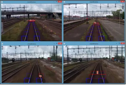
1) Sensitivity equal to 100%. This is a great achievement for safety, because it is essential that false negative do not occur, namely that all the obstacles are identified. Figure 10 shows obstacles of different nature and in different position identified by the system.

2) Ability of the system dealing with shadows. There are many scenes where the lighting conditions are modified by the presence of trees, bridges, and so on. Dealing with shadows is the main reason why we did not choose to apply the Canny method.

3) Ability of the system to get the rail even when the train shakes. Many methods which apply prior knowledge assume the position of the rail in the image is constant, however the train will shake during his journey. This methodology allows to create bottom up windows and to find the rail in

linear time even when a shake occurs between two consecutive frames.

Fig. 10. Obstacles detected on the rail.

and the accelerometer sensor are used to determine if an accident occurred. In the following paragraph a short description of how the method works is presented. Accelerometer sensor data is the main variable which is used to determine if an event has occurred. This is done using a simple algorithm. The main idea is to calculate the differential in kinetic energies between two points. The kinetic energy is equal to the mass of the vehicle multiplied by squared velocity, divided by two:

2 2

V m

E  

The mass m of the vehicle is a constant regardless of the fact the vehicle is carrying passengers, luggage or whatever else and it does not influence the variation of energy:

)

(

V

V

E







In order to get the data from the accelerometer the algorithm is implemented following these steps:

1) The raw data coming from the accelerometer is divided by the three axes x, y, and z. To obtain the acceleration is necessary to sum the three components. The signal is framed into discrete intervals in order to reduce the total amount of data.

2) The velocity is then obtained by integrating the acceleration within the time interval using definite integral. 3) The equation is applied to get the variation of energy.

If the system notes a variation of energy higher than a certain threshold an impact due to an accidental event may have occurred. However, when a vehicle stops or departs from a bus stop, for example, a considerable acceleration/deceleration may be observed, and a false accidental event may wrongly be recorded. For this reason, the GPS is used as support to understand if the variation of energy recorded represents a real accident. If the amount of energy changes in the proximity of a bus stop, for example, the system supposes there is nothing abnormal happened and it does not store the video. On the other hand, if something similar happens into an intersection it is supposed an accident occurred. For this purpose, a handy online tool can be used to create a map of the points of interest , such as bus stops, pedestrian crossings, intersections and so on, for any city in the world. Notwithstanding this measure, the result of the tests carried out on the system presented a significant occurrence of false positive. We find therefore the same drawback of the obstacle detection system and that is why we thought we can apply a similar approach to spot false positive. The idea is to extend the work providing the cameras with processors, in order to make them active devices, able to contribute to the detection of an anomalous situation, not just mere video recorders. We want to analyse a video frame to understand if it shows a traffic accident or not. On the road certainly a wider range of scenarios can be found compared with the railway, where the view is rather monotonous. The algorithm and the classifier we need to apply should be completely different from those used for obstacle detection on railways, but the idea of detecting an anomalous event, in this case a traffic accident, by using computer vision combined with data analysis is very similar.

VI. CONCLUSIONS

This work updates techniques based on prior knowledge and creates an automatic and real time method for obstacles detection on railways. The key contribution are:

1. Except the initialization stage, the system is completely automatic and it does not require the human contribution.

2. It can find the rails in linear time even in critical conditions, which guarantees the real time property of the system.

3. The bottom-up windows are adaptive in position and size and perform well.

The obstacles detection methods have proved to be effective but we need to manage false positive in a better way. Many objects, indeed, can affect the monotony of the images without posing a real danger to the rail journey. Recognition of these objects is essential for a reliable behaviour of the system. Learning and identification of benign object provides interesting challenges for computer vision algorithms. In our particular case, since we use the contours extraction to check for obstacles between the rails, some big metal plates may lead to false positive problems. A solution we are thinking to apply is to collect a large amount of images and to create a dataset composed of positive and negative samples. After that we can use Local Binary Patter to extract features from images and train a Support Vector Machine classifier to be embedded in the system. Another problem we need to solve is identifying crossing areas. In the current work there is no research in this direction, although there are many crossings during the train journey, especially nearby the stations. We hope to manage this problem using one-dimension projection and Gaussian Mixture Model to find the rails correctly in these critical areas.

REFERENCES

[1] Rossi Passarella, Bambang Tutuko, and Aditya PP Prasetyo. Design concept of train obstacle detection system in indonesia. IJRRAS, 9(3):453–460, 2011.

[2] Frank Kruse, Stefan Milch, and Hermann Rohling. Multi sensor system for obstacle detection in train applications. Proc. of IEEE Tr., June, 42–46,2003.

[3] Shigeki Sugimoto, Hayato Tateda, Hidekazu Takahashi, and Masatoshi Okutomi. Obstacle detection using millimeter-wave radar and its visualization on image sequence. In Pattern Recognition, 2004. ICPR 2004. Proceedings of the 17th International Conference on, volume 3, 342–345. IEEE, 2004.

[4] John Canny. A computational approach to edge detection. Pattern Analysis and Machine Intelligence, IEEE Transactions on, (6):679– 698, 1986.

[5] Mei Fang, GuangXue Yue, and Qing-Cang Yu. The study on an application of otsu method in canny operator. In International Symposium on Information

[6] Tingting Yao, Shenghua Dai, Pei Wang, and Yue He. Image based obstacle detection for automatic train supervision. In Image and Signal Processing (CISP), 2012 5th International Congress on, 1267– 1270. IEEE, 2012.E. H. Miller, “A note on reflector arrays (Periodical style—Accepted for publication),” Engineering Letters, to be published.

[7] Lei Tong, Liqiang Zhu, Zujun Yu, and Baoqing Guo. Railway obstacle detection using onboard forward-viewing camera. Journal of Transportation Systems Engineering and Information Technology, 4:013, 2012.

[8] Luis Fonseca Rodriguez, Jonny Alexander Uribe, and Jesus Francisco Vargas Bonilla. Obstacle detection over rails using hough transform. In Image, Signal Processing, and Artificial Vision (STSIVA), 2012 XVII Symposium of, 317–322.IEEE, 2012.

Intelligent Transportation Systems (ITSC), 2012 15th International IEEE Conference on, 1132–1136. IEEE, 2012.

[10] Frederic Maire and Abbas Bigdeli. Obstacle-free range determination for rail track maintenance vehicles. In Control Automation Robotics & Vision (ICARCV), 2010 11th International Conference on, 2172– 2178. IEEE, 2010.

[11] Bruzzone, AG, Mosca, R., Revetria, R., Orsoni, System architecture for integrated fleet management: advanced decision support in the logistics of diversified and geographically distributed chemical processing Proceedings of AIS’02 Conference on AI, Simulation and Planning in High Autonomy Systems pp. 309-314, 2002.le),” IEEE Trans. Electron Devices, vol. ED-11, pp. 34–39, Jan. 1959.

[12] Briano, E., Caballini, C., Revetria, R., The Maintenance Management In The Highway Context: A System Dynamics Approach Proceedings of FUBUTEC, pp. 15-17, 2009.R. W. Lucky, “Automatic equalization for digital communication,” Bell Syst. Tech. J., vol. 44, no. 4, pp. 547–588, Apr. 1965.

[13] Briano, E., Revetria, R., Study of crowd behavior in emergency tunnel procedures, International Journal of Mathematics and Computers in Simulation, Vol. 2, Issue 1, pp. 349-358, 2008. [14] Briano, E., Caballini, C., Revetria, R., Schenone, M., Testa, A., Use

of system dynamics for modelling customers flows from residential areas to selling centers, Proceedings of the 12th WSEAS international conference on Automatic control, modelling & simulation, pp. 269-273, World Scientific and Engineering Academy and Society (WSEAS), 2010..