Exploring the mirror TBA

(1)

arXiv:0911.2224v2 [hep-th] 16 Feb 2010

Preprint typeset in JHEP style - HYPER VERSION ITP-UU-09-54 SPIN-09-44 TCDMATH 09-24 HMI-09-10

Exploring the mirror TBA

Gleb Arutyunova∗†, Sergey Frolovb† and Ryo Suzukib a _{Institute for Theoretical Physics and Spinoza Institute,}

Utrecht University, 3508 TD Utrecht, The Netherlands

b _{Hamilton Mathematics Institute and School of Mathematics,}

Trinity College, Dublin 2, Ireland

Abstract: _{We apply the contour deformation trick to the Thermodynamic Bethe}

Ansatz equations for the AdS5×S5 mirror model, and obtain the integral equations

determining the energy of two-particle excited states dual to _N = 4 SYM operators from the sl(2) sector. We show that each state/operator is described by its own set of TBA equations. Moreover, we provide evidence that for each state there are infinitely-many critical values of ’t Hooft coupling constant λ, and the excited states integral equations have to be modified each time one crosses one of those. In particular, the first critical value for the Konishi operator occurs at λ ≈ 774. Our results disagree with the ones of Gromov, Kazakov and Vieira, and may explain the mismatch between their recent computation of the scaling dimension of the Konishi operator and the one done by Roiban and Tseytlin by using the string theory sigma model.

(2)

1. Introduction

An important open problem of the AdS/CFT correspondence [1] is to understand the finite-size spectrum of the AdS5 ×S5 superstring. Recently, there has been further

(3)

the Konishi operator was computed [2] by means of generalized L¨uscher’s formulae [3, 4, 2] (see also [5]-[15] for other applications of L¨uscher’s approach), and the result exhibits a stunning agreement with a direct field-theoretic computation [16, 17]. Second, the groundwork for constructing the Thermodynamic Bethe Ansatz (TBA) [18], which encodes the finite-size spectrum for all values of the ’t Hooft coupling, has been laid down, based on the mirror theory approach1 _{[20]. Most importantly,}

the string hypothesis for the mirror model was formulated [21] and used to derive TBA equations for the ground state [22]-[25]. Also, a corresponding Y-system [26] was conjectured [27], and its general solution was obtained [28]. The AdS/CFT Y-system has unusual properties, and, in particular, is defined on an infinite-genus Riemann surface [22, 29].

The derivation of the TBA equations is not yet complete, because the equations pertain only to the ground state energy (or Witten’s index in the case of periodic fermions) and do not capture the energies of excited states. Therefore, one has to find a generalization of the TBA equations that can account for the complete spectrum of the string sigma model, including all excited states.

Here we continue to explore the mirror TBA approach. In particular, we will be interested in finding the TBA integral equations which describe the spectrum of string states in the sl(2) sector. An attempt in this direction has been already undertaken in [25] and the emerging integral equations have been used for numerical computation of the anomalous dimension of the Konishi operator [30]. However, the subleading term in the strong coupling expansion in this result disagrees with the result by [31] obtained by string theory means. There exists yet another prediction [32] for this subleading term, which differs from both [30] and [31]. All these results are based on certain assumptions which require further justification. This makes urgent to carefully analyze the issue of the TBA equations for excited states, and to better understand what happens on the string theory side.

In this paper we analyze two-particle states in the sl(2) sector. First, we show that each state is governed by its own set of the TBA equations. Second, we provide evidence that for each state there are infinitely-many critical values of ’t Hooft cou-pling constant λ, and that the excited states integral equations have to be modified each time one of these critical values is crossed.2 _{Performing careful analysis of}

two-particle states in a region between any two neighboring critical points, we propose the corresponding integral equations.

The problem of finite-size spectrum of two-dimensional integrable models has been studied in many works, see e.g. [33]-[49]. To explain our findings, we start

1_{The TBA approach in the AdS/CFT spectral problem was advocated in [19] where it was used} to explain wrapping effects in gauge theory.

(4)

with recalling that for some integrable models the inclusion of excited states in the framework of the TBA approach has been achieved by applying a certain analytic continuation procedure [36, 37]. This can be understood from the fact that the convolution terms entering the integral TBA equations exhibit a singular behavior in the complex rapidity plane, the structure of these singularities does depend on the value of the coupling constant. This leads to a modification of the ground-state TBA equations, which, indeed, describe the profile and energies of excited states. Here we intend a similar strategy for the string sigma model.

To derive the TBA equations for excited states, we propose to use a contour deformation trick. In other words, we assume that the TBA equations for excited states have the same form as those for the ground state with the only exception that the integration contour in the convolution terms is different. Returning the contour back to the real rapidity line of the mirror theory, one picks up singularities of the convolution terms which leads to modification of the final equations. The original contour should be drawn in such a way, that the arising TBA equations would reproduce the large L asymptotic solution.

Recall that the TBA equations for the string mirror model [22] are written in terms of the following Y-functions: YQ-functions associated with Q-particle bound states, auxiliary functions YQ|vw for Q|vw-strings, YQ|w for Q|w-strings, and Y± for

y±-particles. The Y-functions depend on the ’t Hooft couplingλrelated to the string

tension g as λ = 4π2_g2_{. As we will see, the analytic structure of these Y-functions}

depends on g and plays a crucial role in obtaining the TBA equations for excited states.

Most conveniently, the largeLasymptotic solution for the Y-functions is written in terms of certain transfer-matrices associated with an underlying symmetry group of the model [33, 34]. In the context of the string sigma model the corresponding asymptotic solution was presented in [27]. We will use this solution to check the validity of our TBA equations.

Our analysis starts from describing physical two-particle states in thesl(2) sector. It appears that for the sl(2) states the functions YQ|vw(u) play the primary role in

formulating the excited state TBA equations. Analyzing the asymptotic solution, we find that each YQ|vw has four zeroes in the complex u-plane. With g changing, the zeroes change their position as well, and at certain critical values g = gcr they give rise to new singularities in the TBA equations which resolution results in the appearance of new driving terms. The critical values gcr are defined as values of g at which YQ|vw(u) acquires two zeros at u=±i/gcr: YQ|vw(±i/gcr) = 0.

(5)

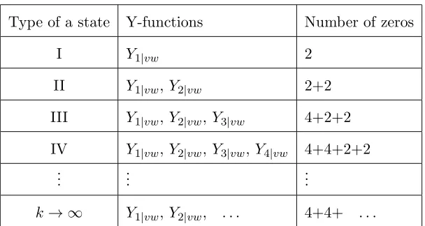
Type of a state Y-functions Number of zeros

I Y₁_|_vw 2

II Y₁_|_vw,Y₂_|_vw 2+2 III Y₁_|_vw,Y₂_|_vw,Y₃_|_vw 4+2+2 IV Y1|vw,Y2|vw,Y3|vw,Y4|vw 4+4+2+2

..

. ... ...

[image:5.612.143.447.81.243.2]

k→ ∞ Y₁_|_vw,Y₂_|_vw, . . . 4+4+ . . .

Table 1. Classification of two-particle states in thesl(2)-sector at g∼0. The right column shows the number of zeros which the corresponding asymptotic

Y_M_|_vw-functions from the middle column have in the physical strip _|Im(u)_|<

1/g. States of type I are called “Konishi-like”. States of type II, III, IV, . . .

correspond to larger value of κ, see section 3.

Each class is unambiguously determined by number of zeroes of YM|vw-functions in

the strip_|Im(u)_|<1/g. In particular, for states of type I onlyY1|vw-function has two

zeroes in the physical strip. We call all these states “Konishi-like” because they share this property with the particular string state corresponding to the Konishi operator. Our results disagree with that by [25, 30] in the following two aspects: First, the integral equations for excited states in the sl(2) sector do not have a universal form, even for two-particle states. Second, we face the issue of critical points. When a critical point is crossed, the compatibility of the asymptotic solution with the integral TBA equations requires modification of the latter. The equations proposed in [25] capture only type I states and only below the first critical point.

To find approximate locations of the critical values, we first solve the asymptotic Bethe-Yang equations [50] (which include the BES/BHL dressing phase [51, 52]) for some states numerically from weak to strong coupling and obtain the corresponding interpolating curve u _≡ u1(g), where u1 is the rapidity of an excited particle in

string theory. The second particle has rapidity u2 =−u1 due to the level matching

condition. Further, we compute the Y-functions on the large L asymptotic solution corresponding to this two-particle excited state and study their analytic properties considered as functions ofg, and, in particular, determine approximately the critical values.

The first critical value for the Konishi operator occurs at λ ≈ 774. In the weak-coupling region below the first critical point, the integral equations for Konishi operator we obtain seem to agree with that of [25]. However, these weak-coupling equations become inconsistent with the known large L asymptotic solution (where

(6)

modified. Consequently, the derivation of the anomalous dimension for the Konishi operator at strong coupling requires re-examination. Of course, the existence of critical points is not expected to violate analyticity of the energy E(λ) of a string state considered as the function of λ, but it poses a question about the precise analytic behavior of E(λ) in the vicinity of critical points.

We discuss both the canonical and simplified TBA equations. The canonical equations [22, 24, 25] follow from the string hypothesis for the mirror model [21] by using the standard procedure, see e.g. [53]. The simplified equations [22, 23] obtained from the canonical ones have more close relation to the Y-system. It turns out that the simplified equations are sensitive only to the critical points defined above. In contrast, the canonical equations have to be modified when crossing not only a critical point but also what we call a subcritical point ¯gcr. A subcritical point ¯gcr is defined as the value of g at which the function YQ|vw(u) acquires zero at u = 0. Hence,

in comparison to the canonical equations, the simplified equations exhibit a more transparent analytic structure. In addition to locality, this is yet another reason why we attribute to the simplified equations a primary importance and carry out their analysis in the main text. To study the exact Bethe equations which determine the exact, i.e. non-asymptotic, location of the Bethe roots, we find it advantageous to use a so-called hybrid form of the TBA equations for YQ-functions. This form is obtained by exploiting both the canonical and simplified TBA equations.

Recently, the finite-gap solutions of semi-classical string theory have been nicely derived [54] from the TBA equations [25]. This raises a question why modifications of the TBA equations we find in this paper were not relevant for this derivation. We have not studied this question thoroughly. However, one can immediately see that there is a principle difference between states with finite number of particles and semiclassical states composed of infinitely many particles. Namely, at strong coupling the rapidities of two-particle states fall inside the interval [₋2,2], while those of semi-classical states are always outside this interval. Thus, the modification of the TBA equations discussed in this paper might not be necessary for semi-classical states. It would be important to better understand this issue.

(7)

-1.0 -0.5 0.5 1.0

-2 2 4

-10 -5 5 10

-3 -2 -1 1 2 3

-10 -5 5 10

[image:7.612.129.468.81.304.2]

-3 -2 -1 1 2 3

Figure 1: These are the mirror and string regions on thez-torus. They are in one-to-one correspondence with the u-planes. The boundaries of the regions are mapped to the cuts.

Finally, in Conclusions we mention some interesting open problems. The definitions, treatment of canonical equations, and further technical details are relegated to eight appendices.

2. Contour deformation trick

The TBA equations for the AdS5×S5 mirror model are written for Y-functions which

depend on the real momentum of the mirror model. The energy of string excited states obviously depends on real momenta of string theory particles, and to formu-late the TBA equations for excited states one also needs to continue analytically the Y-functions to the string theory kinematic region. To visualize the analytic continu-ation it is convenient to use the zQ-tori because the kinematic regions of the mirror and string theory Q-particle bound states (Q-particles for short) are subregions of thez-torus, see Figure 1. In addition, the Q-particle energy, and many of the kernels appearing in the set of TBA equations are meromorphic functions on the correspond-ing torus. The mirror Q-particle region can be mapped onto au-plane with the cuts running from the points _±2_± i

gQ to ±∞, and the string Q-particle region can be mapped onto a u∗-plane with the cuts connecting the points −2± _giQ and 2± _giQ,

see Figure 1. Since the cut structure on the planes is different for each Y-function, they cannot be considered as different sheets of a Riemann surface. The zQ-torus can be glued either from four mirroru-planes or four string u∗-planes.

(8)

imaginary period of the torus

z =z∗+

ω2

2 , (2.1)

wherez is the variable parametrizing the real momenta of the mirror theory, andz∗ is

the variable parametrizing the real momenta of the string theory. The line (_−∞,_∞) in the string u∗-plane is mapped to the interval Re(z∗) ∈ (−ω₂1,ω₂1), Im(z∗) =const

on the z-torus, and we choose z∗ in the string region to be real. Then, the interval

Re(z) ∈ (−ω1

2 ,

ω1

2 ), Im(z) =

ω2

2i of the mirror region is mapped onto the real line of the mirror u-plane.

It is argued in [36, 37] that the TBA equations for excited states can be obtained from the ones for the ground state by analytically continuing in the coupling constants and picking up the singularity of proper convolution terms. We prefer however to employ a slightly different procedure which we refer to as the contour deformation trick. We believe it is equivalent to [36, 37]. It is based on the following assumptions

• The form of TBA equations for any excited state and the expression for the energy are universal. TBA equations for excited states differ from each other only by a choice of integration contours of convolution terms and the length parameter L which depend on a state.

• The choice of the integration contours andLis fixed by requiring that the large

L solution of the excited state TBA equations be given by the generalized L¨uscher formulae, that is all the Y-functions can be written in terms of the eigenvalues of the transfer matrices. The integration contour depends on the excited state under consideration, and in general on the values of ’t Hooft’s coupling andL.

• An excited state is completely characterized by the five charges it carries and a set ofN real numberspkwhich are in one-to-one correspondence with momenta

po

k of N Q-particles in the small coupling limit g → 0. The momenta pok are found by using the one-loop Bethe equations for fundamental particles and their bound states. For finite values of g the set of pk is determined by exact Bethe equations which state that at anyp=pkthe correspondingYQ-functions are equal to ₋1.

We consider only the simplest case of two-particle excited states in the sl(2) sector of the string theory because there are no bound states in this sector and the complete two-particle spectrum can be readily classified. The physical states satisfy the level-matching condition which for two-particle states takes a very simple form:

p1 =−p2, or u1 =−u2, orz∗1 =−z∗2 depending on the coordinates employed. The

(9)

3. States and Y-functions in the

sl

(2)

sector

To fix the integration contour one should choose a state and analyze the analytic structure of the largeLY-functions which we refer to as the asymptotic Y-functions. We begin with a short discussion of two-particle states in the sl(2) sector.

3.1 Bethe-Yang equations for the sl(2) sector

There is only a single Bethe-Yang (BY) equation in thesl(2)-sector for two-particle physical configurations satisfying the vanishing total momentum conditionp1+p2 = 0

that can be written in the form [55]

1 = eipJSsl(2)(p,−p) =⇒ eip(J+1) =

1 + 1

x+s2

1 + _x−1

s2

σ(p,−p)2, (3.1)

where p≡p1 >0, J is the charge carried by the state, σ is the dressing factor, and

x±

s are defined in appendix 8.1. Taking the logarithm of the equation, one gets

ip(J + 1)₋log1 +

1

x+s2

1 + _x−1

s2

−2i θ(p,₋p) = 2πi n , (3.2)

where θ = 1

i logσ is the dressing phase, and n is a positive integer because we have assumed p to be positive. As was shown in [56], at large values of g the integer n is equal to the string level of the state.

As is well known, in the small g limit the equation has the obvious solution

po_J,n = 2πn

J + 1, n = 1, . . . ,

J+ 1 2

, (3.3)

where [x] denotes the integer part of x, and the range of n is bounded because the momentum p can only take values from 0 to π. The corresponding rapidity variable

uJ,n in the small g limit takes the following form

uJ,n → 1

gu

o

J,n, uoJ,n= cot

πn

J + 1. (3.4)

Thus, any two-particle state in the sl(2) sector is completely characterized by the two integers J and n. In particular, in the simplest J = 2 case corresponding to a descendent of the Konishi state n can take only one value n = 1, and the small g

solution is

po₂_,₁ = 2π 3 , u

o

2,1 =

1

√

3. (3.5)

(10)

[image:10.612.88.515.79.224.2]

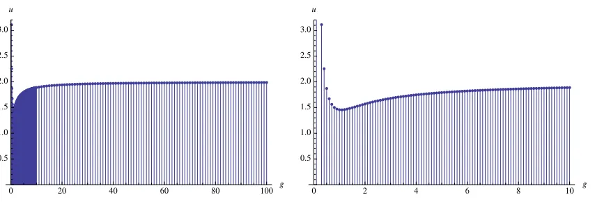
Figure 2: These are the plots of u which solves the BY equation for the Konishi state.

representation [51] for the dressing phase for perturbative computations, and the DHM integral representation [57] for the numerical ones3_{. For the Konishi state, the}

perturbative solution up to g16_{-th can be found in appendix 8.2.}

We have solved numerically the BY equation for the Konishi state for ₁₀1 ≤g ≤

1000 with the step ₁₀1 for ₁₀1 ≤ g ≤ 10, the step 1 for 10 ≤ g ≤ 100, and the step 10 for 100_≤ g _≤ 1000. In Figure 2 we show the results up to g = 100. For greater values of g nothing interesting happens, and the solution can be approximated by asymptotic formulae from [56, 32, 58], see appendix 8.2 for more details. We then applied the Interpolation function in Mathematica to haveu2,1 as a smooth function

of g. Using the function, one can find thatu2,1(g) decreases up to g ∼0.971623, and

then begins to increase and at large g it asymptotes to u= 2.

The functionsuJ,n(g) for other values ofJ andnhave similarg dependence. The only exception is the case J = 2n₋1 where the exact solution of the BY equation isp2n−1,n =π and, therefore, u2n−1,n = 0. The TBA equations we propose below are not in fact valid for these (2n−1, n) states.

The perturbative and numerical solutions foruJ,n(g) can be easily used to analyze the behavior of Y-functions considered as functions of g. In particular it is easy to determine if some of them become negative for large enough values of g.

3.2 Y-functions in the sl(2) sector

Let us recall that the TBA equations for the AdS5 ×S5 mirror model involve Y

Q-functions for momentum carrying Q-particle bound states, and auxiliary functions

Y_Q(α_|_vw) for Q|vw-strings, Y_Q(α_|_w) for Q|w-strings, and Y±(α) for y±-particles. The index

α= 1,2 reflects twosu(2|2) algebras in the symmetry algebra of the light-cone string sigma model. The TBA equations [22] depend also on the parameters hα which take care of the periodicity condition of the fermions of the model [59]. For thesl(2) sector

(11)

the fermions are periodic, and from the very beginning one can set the parametershα to 0 because there is no singularity athα = 0 in the excited states TBA equations.

For the sl(2) states there is a symmetry between the left and right su(2_|2) aux-iliary roots, and, therefore, all Y-functions satisfy the condition

Y_∀(1) =Y_∀(2) =Y∀, (3.6)

where _∀ denotes a Y-function of any kind.

The string theory spectrum in thesl(2) sector is characterized by a set of N real numbersz∗k orukcorresponding to momenta ofN fundamental particles in the limit

g → 0. According to the discussion above, these numbers are determined from the exact Bethe equations

Y1(z∗k) =Y1∗(uk) =−1, k = 1, . . . , N , (3.7)

whereY1(z) is the Y-function of fundamental mirror particles considered as a function

on thez-torus, andY1∗(u) denotes theY1-function analytically continued to the string

u-plane.

In the largeJ limit the exact Bethe equations must reduce to the BY equations, and it is indeed so because the asymptoticsl(2)YQ-functions can be written in terms of the transfer matrices defined in appendix 8.3 as follows [2]

Y_Qo(v) =e−JEeQ(v) TQ,1(v|~u)

2

QN

i=1S 1∗Q

sl(2)(ui, v)

=e−JEeQ(v)_T

Q,1(v|~u)2

N

Y

i=1

SQ1∗

sl(2)(v, ui), (3.8)

where v is the rapidity variable of the mirror u-plane and _EeQ is the energy of a mirror Q-particle. S1∗Q

sl(2) denotes the S-matrix with the first and second arguments

in the string and mirror regions, respectively. TQ,1(v|~u) is up to a factor the trace of

the S-matrix describing the scattering on these string theory particles with a mirror Q-particle or in other words the eigenvalue of the corresponding transfer matrix. The BY equations then follow from the fact that _Ee1∗(uk) =−ipk, and the following

normalization of T1,1

T1,1(u∗k|~u) = 1 =⇒ −1 =e

iJpk

N

Y

i=1

S1∗1∗

sl(2)(uk, ui), (3.9)

whereu∗k =uk, and the star just indicates that one analytically continuesT1,1 to the

string region. Then, S1∗1∗

sl(2)(uk, ui) = Ssl(2)(uk, ui) is the usual sl(2) sector S-matrix used in the previous subsection.

Let us also mention that TQ,1 has the following large v asymptotics

TQ,1(v|~u)→Q 1−

N

Y

i=1

s

x+_i x−_i

!2

(12)

and therefore it goes to 0 if the level-matching is satisfied.

Then, in the large J limit all auxiliary asymptotic sl(2) Y-functions can be written in terms of the transfer matrices as follows [27]

Y₋o = −T2,1

T1,2

, Y₊o =−T2,3T2,1

T3,2T1,2

, Y_Qo_|_vw = TQ+2,1TQ,1

TQ+1,2

, Y_Qo_|_w = T1,Q+2T1,Q

T2,Q+1T0,Q+1

.

The transfer matrices Ta,s can be computed in terms ofTa,1 by using the

Bazhanov-Reshetikhin formula [61], see appendix 8.3 for all the necessary explicit formulae. An important property of the Y-functions for vw- and w-strings is that they approach their vacuum values as v _{→ ∞}

YM|vw(v)→M(M + 2), YM|w(v)→M(M+ 2), v → ∞, −

M

g <Im(v)< M

g .

Now we are ready to analyze the dependence of asymptotic Y-functions on g. Recall that they depend on the rapiditiesuk which are solutions of the BY equations. We begin with the small g limit where the effective length goes to infinity, and one can in fact trust all the asymptotic formulae. It is convenient to rescale v anduk variables asv _→v/g,uk →uk/gbecause the rescaled variables are finite in this limit. Let κ ≡u1 =−u2 be the rescaled rapidity of a fundamental particle. According to

the previous subsection, in the small g limit they are given by uo

J,n, eq.(3.4).

The most important functions in the sl(2) case are YM|vw, and we find that for

N = 2 they exhibit the following small g behavior in the strip−M <Im(v)< M

Y_M_|_vw(v) =M(M+ 2)

M2₋_{1 +}_v2₋_κ2₍_M_{+ 2)}2₋_{1 +}_v2₋_κ2

(M + 1)2_{+ (}_v₋_κ₎2₍_M _{+ 1)}2_{+ (}_v₊_κ₎2 +O(g

2₎_. _(3.11)

The leading term has the correct largeu-asymptotics and four apparent zeros at

v =_±√κ2 ₋_M2_{+ 1}_, _v ₌_±p_κ2₋₍_M _{+ 2)}2_{+ 1}_.

One can see thatY1|vw-function always has at least two real zeros at v =±κ. Other

zeros of YM|vw-functions can be either real or purely imaginary depending on the

values of M and κ. It appears that the form of simplified TBA equations depends on the imaginary part of these zeros, and we will see in next sections that if a pair of zeros v =_±r fall in the strip _|Im(r)_|<1 then the equations should be modified.

Thus, we are lead to consider the following three possibilities

1. IfM2₋₂_{< κ}2 _<₍_M₊₂₎2₋_{2 then}_Y

M|vwhas two zeros atv =±

√

κ2₋_M2_{+ 1}

that are in the strip_|Im(v)_|<1. In terms of the integersJandmcharacterizing two-particle states one gets the condition

√

M2 ₋₂_<_cot πn

J + 1 <

p

(13)

2. Ifκ2 _{< M}2 ₋₂ _⇐⇒ _cot πn J+1 <

√

M2₋_{2 then} _Y

M|vw does not have any zeros in the strip |Im(v)|<1.

3. Ifκ2 _>₍_M_{+ 2)}2₋₂ _⇐⇒ _cot πn J+1 >

p

(M + 2)2₋_{2 then}_Y

M|vwhas four zeros in the strip |Im(v)|<1.

Some of these zeros can be real, and in fact the canonical TBA equations take different forms depending on whether the roots are real or imaginary.

Classification of two-particle states atg ∼0 is presented in Table 1. The type of a state is determined by how many zeroes of YM|vw-functions occur in the physical strip and it depends on J and n.

Consider a two-particle state with κ=uo

J,n for some (J, n). Table 1 shows that there exists a number m_≥1, equal to the maximal value of M the condition (3.12) is satisfied. Then both Ym|vw and Ym−1|vw have two zeros, all Yk|vw with k ≤m−2 have four zeros, and all Yk|vw-functions with k ≥ m+ 1 have no zeros in the strip

|Im(v)_| < 1. For example, among the states with (J, n = 1) at small coupling, the states of type I are found if and only if J ≤ 7. The type II is found for 5≤ J ≤7, type III for 8 ≤ J ≤ 11, and type IV for 12 ≤ J ≤ 14. In particular, Y1|vw for the state (8,1) has two real zeros and two imaginary zeros in the strip_|Im(v)_|<1, and

Y1|vw for the state (J ≥9,1) has four real zeros.

As for the Konishi state with J = 2 and n = 1 only Y1|vw-function has two

zeros and all the other YM|vw-functions have no zeros at small coupling. Let us also mention that at g = 0 the Y2|vw-function of the state (5,1) (and in general of any state (6k₋1, k)) has a double zero atv = 0. This double zero however is an artifact of the perturbative expansion, and in realityY2|vw has two imaginary zeros for small values of g equal to ≈ ±ig√3. For the state with J = 6 and n = 1 both Y1|vw and

Y2|vw have two real zeros.

3.3 Critical values of g

Evolution of zeros

Now we would like to understand what happens withYM|vw-functions when one starts

increasing g. To this end one should use numerical solutions of the BY equations discussed at the beginning of this section. We also switch back to the original u

variables because they are more convenient for general values of g, and refer to the strip _|Im(u)_|<1/g as the physical one.

We find that for finite g any Yk|vw-function has four zeros which are either real or purely imaginary. We could not find any other complex zeros. The four zeros of

(14)

are the zeros ofYk|vw which have a larger absolute value than ˆrj(k). If only two zeros are real then we denote them as r(_jk) and the imaginary zeros as ˆr_j(k). Finally, if the four zeros are imaginary thenr_j(k)are the ones closer to the real line than the second pair ˆr_j(k).

The locations of the zeros depend on g, and we should distinguish two cases. We observe first that if two zeros are real at g ∼ 0 then they are of order 1/g, and obviously outside the interval [₋2,2]. With g increasing they starts moving toward the origin, and at some value ofg they reach their closest position to the origin which is inside the interval [₋2,2]. Then, for larger g they remain inside the interval but begin to move to its boundaries and reach them at g =∞. In the second case, one considers a pair of imaginary zeros at g ∼ 0. With g increasing they start moving toward the real line, and at some value of g they get to the origin and become a double zero. Then, for largerg they split and begin to move to the boundaries of the interval [₋2,2], and reach them atg =_∞. The only exception from this behavior we find is the g-dependence of the two zeros of Y2|vw-function for the states (6k−1, k)

that are equal to±i√3 at small g. These zeros become real at very small value ofg. Then they start moving to±2, cross the boundaries of the interval [−2,2], and reach their maximum. After that they behave as zeros of all the other Yk|vw-functions.

Thus, at very large values of g all zeros of any Yk|vw-function are real, inside the interval [₋2,2], and very close to_±2.

The pairs of the zeros of different YM|vw-functions are not independent, and satisfy the following relations

ˆ

r_j(k−1) =r_j(k+1), k = 2, . . . ,∞. (3.13)

Therefore, the zeros of YM|vw-functions can be written as follows

{r(1)_j , r_j(3)_};_{r_j(2), r(4)_j _};. . .;_{r_j(k−1), r_j(k+1)_};_{r_j(k), r_j(k+2)_};_{r_j(k+1), r_j(k+3)_};. . . ,(3.14)

so that Yk|vw has the zeros {rj(k), r

(k+2)

j }.

These zeros have a natural ordering. If we assume for definiteness that the zeros with j = 1 have negative real or imaginary parts, then they are ordered as

r₁(1) _≺r₁(2) _≺r(3)₁ _{≺ · · · ≺}r₁(k) _≺r(₁k+1) _{≺ · · ·} , (3.15)

where r₁(k) ≺ r₁(k+1) if either Re(r₁(k)) < Re(r₁(k+1)) or Im(r₁(k)) > Im(r(₁k+1)). It is important that the zeros never change the ordering they have atg ∼0. In particular,

(15)

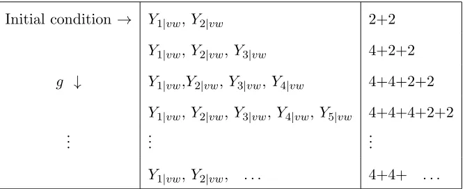
Initial condition_→ Y₁_|_vw,Y₂_|_vw 2+2

Y1|vw,Y2|vw,Y3|vw 4+2+2 g _↓ Y₁_|_vw,Y₂_|_vw,Y₃_|_vw,Y₄_|_vw 4+4+2+2

Y1|vw,Y2|vw,Y3|vw,Y4|vw, Y5|vw 4+4+4+2+2

..

. ... ...

[image:15.612.131.465.83.219.2]

Y1|vw,Y2|vw, . . . 4+4+ . . .

Table 2. Evolution of a two-particle states in the sl(2)-sector with respect to g. At g ∼0 a state has a certain number of YM|vw-functions with zeroes

in the physical strip. Increasing the coupling, the critical points get crossed which leads to accumulation of zeroes of Y_M_|_vw’s in the physical strip. This phenomenon can be called “Y-function democracy”.

In addition we find that the functions below have either zeros or equal to₋1 at locations related to r(_jk)

Yk|vw r(jk+1)±

i g

=₋1, Yk+1 r(jk+1)

= 0, k = 1, . . . ,_∞, Y± r(2)j

= 0.(3.16)

As will be discussed in the next section the equations Yk|vw rj(k+1)±gi

=−1 lead to integral equations which play the same role as the exact Bethe equationsY1(uj) =−1 and allow one to find the exact location of the rootsr_j(k+1).

Let us finally mention that nothing special happens toYM|w-functions.

Critical and subcritical values

Letmagain be the maximum value ofM the condition (3.12) is satisfied. According to the discussion above for any two-particle state there is a critical value of g such that the function Ym+1|vw which had no zeros in the physical strip for small values of g, acquires two zeros at u= ±i/g. At the same time Ym−1|vw also acquires zeros at u = _±i/g. At a slightly larger value of g the two zeros that were at u = _±i/g

This pattern repeats itself, and there are infinitely many critical values ofg which we denote as g_J,nr,m and define as the smallest value of g such that for a symmetric configuration of Bethe roots the function Ym+r|vw acquires two zeros at u = ±i/g. The subscript J, n denotes a state in the sl(2) sector, and they determinem.

The critical values ofg can be also determined from the requirement that atg =

(16)

This condition is particularly useful because the value of the Y-functions at u = 0 can be found from the TBA equations, see next section for detail.

The second set of subcritical values ofg can be defined as the smallest value of g

such that the function Ym+r|vw acquires a double zero atu= 0. They are denoted as ¯

g_J,nr,m, and they are always greater than the corresponding critical values: g_J,nr,m<g¯r,m_J,n. The locations of the critical values depend on the state under consideration, and can be determined approximately by using the asymptotic Y-functions discussed in the previous subsection. The values obtained this way are only approximate because for large enough values of g one should take into account the deviations of the Y-functions from their large J expressions. Since at very large values of g the contribution of YQ-functions to the exact energy is expected to be negligible,4 _these

values should also be accurate enough for any J at strong coupling.

We will see in next sections that the critical values g_J,nr,m play a crucial role in formulating excited states simplified TBA equations which take different form in each of the intervals g_J,nr,m < g < g_J,nr+1,m, r= 0,1, . . . where g_J,n0,m = 0. The second set of ¯gr,m_J,n is not important for the simplified equations. The canonical TBA equations however require both sets because they take different form in each of the intervals

g_J,nr,m < g <g¯_J,nr,m; ¯g_J,nr,m < g < gr_J,n+1,m, r = 0,1, . . ..

Strictly speaking the integration contour in TBA equations also depends on g

and the state under consideration. Nevertheless it appears that in simplified TBA equations the contour can be chosen to be the same for all values of g, and even for all two-particle states from the sl(2) sector if one allows its dynamical deformation. That means that with increasing g the contour should be deformed in such a way that it would not hit any singularity. This also shows that one should not expect any kind of non-analyticity in the energy of a state at a critical value of g. What may happen is that the critical values are the inflection points of the energy.

Critical values of g for the Konishi state

In this subsection we discuss in detail the critical values for Konishi state. To analyze the dependence of Y-functions on g one should first solve the BY equations with

J = 2, n = 1, and then plug the uj’s obtained into the expressions for Y-functions from appendix 8.3.

Solving the equations

Yr+1|vw(±

i

g, g) = 0, r= 1,2, . . . , (3.17)

we find that there are 7 critical values of g for g <100

g₂(r,_,₁1) =_{4.429,11.512,21.632,34.857,51.204,70.680,93.290_}. (3.18)

(17)

[image:17.612.96.502.79.207.2]

Figure 3: On the left and right picturesY1|vw,Y2|vwand Y3|vw are plotted for the Konishi

state at ¯gcr(1) ≈4.5 and ¯g(2)cr ≈11.5, respectively. Y2|vw touches the u-axis atg = ¯g(1)cr , and

has two real zeros for ¯g(1)cr < g <¯gcr(2).

Note that the distance between the critical values increases withg. The first critical value is distinguished because only Y2|vw(±i/g, g) vanishes there. For all the other critical values the function Yr−1|vw(±i/g, g) also is equal to zero

Yr+1|vw(±

i g, g

(r,1)

2,1 ) = 0 =⇒ Yr−1|vw(±

i g, g

(r,1)

2,1 ) = 0, for r = 2,3, . . . . (3.19)

Then, solving the equations

Yr+1|vw(0, g) = 0, r= 1,2, . . . , (3.20)

one finds the following 7 subcritical values of g for g <100

¯

g₂(r,_,₁1) ={4.495,11.536,21.644,34.864,51.209,70.684,93.292}. (3.21)

Note that the distance between a critical value and a corresponding subcritical one decreases with g. Again, at the first subcritical value only Y2|vw(0, g) vanishes. For

all the other subcritical values the functionYr−1|vw(0, g) also acquires an extra double zero

Yr+1|vw(0,g¯2(r,,11)) = 0 =⇒ Yr−1|vw(0,g¯(2r,,11)) = 0, for r = 2,3, . . . . (3.22)

Onceg crosses a subcritical value ¯g(2r,,11) the corresponding double zeros at u= 0 split,

and each of the functions Yr−1|vw(0, g) and Yr+1|vw(0, g) acquires two symmetrically located zeros. As a result at infinite g all the YM|vw-functions have four real zeros.

Moreover, one can also see that if g is between two subcritical values then all these zeros for all the functions are inside the interval [−2,2] and approach ±2 asg → ∞.

In Figures 3-5, we show several plots ofYM|vw-functions for the Konishi state.

In what follows a Konishi-like state refers to any two-particle state for which only

(18)

[image:18.612.96.502.80.209.2]

at g= ¯g(2)cr , andY2|vw andY4|vw touch it atg= ¯g(3)cr . Y1|vw has four real zeros for g >g¯(2)cr .

Figure 5: On the left picture and right picturesY2|vw, Y3|vw,Y4|vw and Y5|vw are plotted

Critical values of g for some states

Here we analyze theg-dependence of Y-functions for several other states.

We begin with the state withJ = 5 andn = 1. This is the state with the lowest value ofJ such that bothY1|vw andY2|vwhave two zeros in the physical strip at small

g. The critical and subcritical values are determined by the equations

Yr+2|vw(±

i

g, g) = 0, Yr+2|vw(0,g¯) = 0, r= 1,2, . . . , (3.23)

and we find the following values for g <100

g₅r,_,2₁ = _{6.707,15.458,27.233,42.107,60.101,81.222_} (3.24) ¯

g₅r,_,2₁ = {6.764,15.479,27.244,42.114,60.105,81.225}.

[image:18.612.87.504.236.413.2]

(19)

has two imaginary zeros in the physical strip at small g. Therefore, the critical and subcritical values are determined by the equations

Yr+3|vw(±

i

g, g) = 0, Yr+2|vw(0,g¯) = 0, r= 1,2, . . . . (3.25)

We find the following 6 critical and 7 subcritical values ofg for g <100

g₈r,_,3₁ = _{{ −} ,9.157,19.561,32.985,49.505,69.143,91.909_} (3.26) ¯

g8r,,31 = {0.116,9.207,19.580,32.995,49.511,69.148,91.912}.

The reason why g1₈_,,3₁ is so small is that the two imaginary roots of Y3|vw that are in the physical strip at g = 0 reach the real line very quickly.

One might think that the first critical value increases withJ. It is not so as one can see on the example of the state with J = 9 and n = 1. This is again the state such that Y1|vw has four zeros, and Y2|vw and Y3|vw have two zeros at small g, and it has the following 6 critical values of g for g <100

g9r,,31 = {6.970,16.982,29.935,45.968,65.114,87.384} (3.27)

¯

g₉r,_,3₁ = {7.052,17.006,29.947,45.976,65.119,87.388}.

4. TBA equations for Konishi-like states

As was discussed above to formulate excited state TBA equations one should choose an integration contour, take it back to the real line of the mirror plane, and then check that the resulting TBA equations are solved by the largeL expressions for Y-functions. We begin our analysis with the simplest case of a Konishi-like state which appears however to be quite general and allows one to understand the structure of the TBA equations for any two-particlesl(2) sector state. To simplify the notations we denote the critical values of the state under consideration asgcr(r).

4.1 Excited states TBA equations: g < gcr(1)

Let us stress that the equations below are valid only for physical states satisfying the level-matching condition. Since some terms in the equations below have the same form for anyN we keep an explicit dependence on N in some of the formulae.

Integration contour

The integration contour for all Y-functions but Y± is chosen in such a way that it

lies a little bit above the interval Re(z)∈(−ω1

2 ,

ω1

2 ), Im(z) =

ω2

2i in the middle of the mirror theory region, and penetrates to the string theory region in the small vicinity ofz=ω2/2 (the centre point of the mirror region). Then, it goes along the both sides

(20)

[image:20.612.112.487.79.279.2]

Figure 6: On the left picture the integration contour on the z-torus is shown. On the right picture a part of the integration contour on the mirror u-plane going from_±∞a little bit above the real line to the origin, and down to the string region is plotted. The green curves correspond to the horizontal lines on the z-torus just above the real line of the string region. The red semi-lines are the cuts of the mirror u-plane, and on the z-torus they are mapped to the part of the boundary of the mirror region that lies in the string region.

that they lie between the mirror theory line and the integration contour, see Figure 6. In the mirror u-plane the contour lies above the real line, then it goes down at

u=_±0, reaches a minimum value and turns back to the real line. In the equations involving the functions YQ, YQ|vw and YQ|w it crosses the cuts of the mirror u-plane with Im(u) = ₋Q_g, and enters another sheet, see Figure 2. It is worth mentioning that the contour does not cross any additional cutsY-functions have on the z-torus. Then, one uses the TBA equations for the ground state energy, and taking the integration contour back to the mirror region interval Im(z) = ω2

2i, picks up N extra contributions of the form₋logS(z∗, z) from any term log(1 +Y1)⋆ K, where S(w, z)

is the S-matrix corresponding to the kernel K: K(w, z) = 1 2πi

d

dwlogS(w, z). In addition, one also gets contributions of the form −logS(w, z) from the imaginary zeros of 1 +YM|vw located below the real line of the mirror u-plane, see (3.16).

Finally, the integration contour forY±-functions should be deformed so that the

pointsu−_k =uk−_gi of the mirroru-plane lie between the interval [−2,2] of the mirror theory line and the contour. Then, the terms of the form log(1₋Y+) ˆ⋆ K would

produce extra contributions of the form + logS(u−_k, z) because Y+(u−k) = ∞. In fact, this is important only if one uses the simplified TBA equations because in the canonical TBA equationsY±-functions appear only in the combination 1−_Y1_±. Note

also thatY±-functions analytically continued to the whole mirroru-plane have a cut

(21)

as was shown in [22], is necessary for the fulfillment of the Y-system

Y+(u±i0) =Y−(u∓i0) for u∈(−∞,−2]∪[2,∞). (4.1)

This equality shows that one can glue the two u-planes along the cuts, and then

Y±-functions can be thought of as two branches of one analytic function defined on

the resulting surface (with extra cuts in fact). We will see that the equality (4.1) indeed follows from the TBA equations.

Simplified TBA equations

Using this procedure and the simplified TBA equations for the ground state derived in [22, 23], one gets the following set of integral equations for Konishi-like states and

g < gcr(1)

• M|w-strings: M ≥1 , Y0|w = 0

logYM|w = log(1 +YM−1|w)(1 +YM+1|w)⋆ s+δM1 log

1− 1

Y−

1− 1

Y+

ˆ

⋆ s . (4.2)

These equations coincide with the ground state ones.

• M_|vw-strings: M _≥1 ,Y0|vw = 0

logYM|vw(v) = −δM1

N

X

j=1

logS(u−_j −v)−log(1 +YM+1)⋆ s (4.3)

+ log(1 +YM−1|vw)(1 +YM+1|vw)⋆ s+δM1log

1−Y−

1₋Y+

ˆ

⋆ s ,

where u−

j ≡ uj − _gi, and the kernel s and the corresponding S-matrix S are defined in appendix 8.1. For M = 1 the first term is due to our choice of the integration contour for Y±-functions, and the pole ofY+ atu=u−j.

It is worth pointing out that there is no extra contribution in (4.3) from any term of the form log(1 +Yk|vw)⋆ s. In general such a term leads to a contribution equal to₋logS(r1−v)S(r2−v) wherer1 and r2 are the two zeros of 1 +Yk|vw with negative imaginary parts. To explain this, we notice that if the zerosr_j(k+1)ofYk+1|vw lie outside the physical strip, then rj are r1 =r1(k+1)− gi and r2 =r

(k+1)

1 + gi, where Im(r(₁k+1)) < ₋1

g. Since S(r− i

g)S(r+ i

(22)

[image:22.612.104.489.92.625.2]

Figure 7: In the upper pictures the positions of zeros of Yk+1|vw and of 1 +Yk|vw are

shown forg < gcr. The contributions of log(1 +Yk|vw)⋆ sto the TBA equations cancel out

for this case. The two pictures in the middle correspond to the situation when two zeros of

Yk+1|vw enter the physical region |Imu|< 1_g (depicted in yellow). Finally, the two pictures

at the bottom are drawn for the case when two zeros of Y_k₊₁_|_vw are on the real line which corresponds togcr <¯gcr < g. Wheng > gcr the contributions of log(1 +Yk|vw)⋆ sdo not

(23)

On the other hand, if the zerosr(_jk+1) ofYk+1|vw lie inside the physical strip then

rj are related tor(jk+1) asrj =rj(k+1)−gi, and the term log(1 +Yk|vw)⋆ s leads to the extra contribution equal to −PjlogS(r

(k+1)−

j −v) where r

(k+1)−

j ≡ r

(k+1)

j − gi, see Figure 7.

We conclude therefore that at weak coupling and only for Konishi-like states no term log(1+Yk|vw)⋆sgives an extra contribution to the TBA equations forvw-strings. Let us also mention that the poles of S(u−_j ₋v) cancel the zeros of Y1|vw(v) at

v =uj, and (4.3) is compatible with the reality condition for Y-functions.

• y-particles 5

logY+

Y−

(v) = −

N

X

j=1

logS1∗y(uj, v) + log(1 +YQ)⋆ KQy, (4.4)

logY+Y−(v) = −

N

X

j=1

log S

1∗1

xv

2

S2

⋆ s(uj, v) (4.5)

+ 2 log1 +Y1|vw 1 +Y1|w

⋆ s−log (1 +YQ)⋆ KQ+ 2 log(1 +YQ)⋆ KxvQ1⋆ s ,

where we use the following notation

log S

1∗1

xv

2

S2

⋆ s(uj, v)≡

Z ∞

−∞

dtlog S

1∗1

xv (uj, t)2

S2(uj−t)

s(t₋v).

Then, S1∗y(uj, v) ≡ S1y(z∗j, v) is a shorthand notation for the S-matrix with the

first and second arguments in the string and mirror regions, respectively. The same convention is used for other S-matrices. Both arguments of the kernels in these formulae are in the mirror region.

Taking into account that under the analytic continuation through the cut_|v_|>2 the S-matrixS1∗y and the kernelKQy transforms asS1∗y →1/S1∗yandKQy → −KQy,

one gets that the functions Y± are indeed analytic continuations of each other and,

therefore, the equality (4.1) does hold.

It can be easily checked that the term on the first line in (4.5) is real, and this makes obvious that the equations for Y±-functions are also compatible with the

reality of Y-functions. The origin of this term can be readily understood if one uses the following identity

−log S

1∗1

xv

2

S2

⋆ s(uj, v) = logS1(uj−v)−2 logSxv1∗1⋆ s(uj, v) (4.6)

5_{The equation for}_Y

+Y− follows from eq.(4.14) and (4.26) of [22], and the identity

KQyˆ⋆ K1 =KxvQ1−KQ−1. Another identity KxvQ1⋆ s= 21KQy+1₂KQ−δQ1s−KQymsˇ⋆˜s , where ˜

s(u)_≡s(u₋ i

(24)

which holds up to a multiple of 2πi, and since S1∗1

xv (u, v) has a zero at u = v the integration contour in the second term on the r.h.s. of (4.6) runs above the real line. Then, the term logS1(uj−v) comes from the term −log (1 +Y1)⋆ K1, and the

second term come from 2 log(1 +Y1)⋆ KxvQ1⋆ s.

Eq.(4.5) is very useful for checking the TBA equations in the largeJ limit where one gets

logY+Y− = −

N

X

j=1

log S

1∗1

xv

2

S2

⋆ s(uj, v) + 2 log

1 +Y1|vw 1 +Y1|w

⋆ s .

• Q-particles for Q_≥3

logYQ = log

1 + _Y 1

Q−1|vw

2

(1 + 1

YQ−1)(1 +

1

YQ+1)

⋆ s (4.7)

• Q= 2-particle

logY2 =

N

X

j=1

logS(uj −v)−log(1 + 1

Y1

)(1 + 1

Y3

)⋆ s+ 2 log

1 + 1

Y1|vw

⋆ s (4.8)

In fact by using the p.v. prescription, one gets

logY2 = log

1 + _Y 1

1|vw

2

(1 + _Y1

1)(1 +

1

Y3)

⋆p.v.s (4.9)

which makes obvious the reality of Y-functions.

• Q= 1-particle

logY1 =

N

X

j=1

log ˇΣ2₁_∗Sˇ1ˇ⋆ s(uj, v)−LEˇˇ⋆ s+ log

1− 1

Y−

2

Y2ˆ⋆ s

− 2 log

1− 1

Y−

1− 1

Y+

Y2ˆ⋆Kˇˇ⋆ s+ logY1⋆Kˇ1ˇ⋆ s

− log (1 +YQ)⋆ 2 ˇKQΣ+ ˇKQ+ ˇKQ−2

ˇ

⋆ s−log(1 +Y2)⋆ s . (4.10)

All the kernels appearing here are defined in appendix 8.1, and we also assume that ˇ

K0 = 0 and ˇK−1 = 0. The reality of this equation follows from the reality of

Sss(u− i g, v)2 ˇ

S1(u, v)

= xs(u− i

g)−xs(v)

xs(u₋_gi)₋ _x1

s(v)

xs(u+_gi)−xs(v)

xs(u+_gi)₋ _x1

s(v)

=Sss(u₋ i

(25)

which appears if one uses the representation (8.24) for ˇΣ1∗. Note that ˇS1(u, v) is

defined through the kernel ˇK1(u, v) by the integral

ˇ

S1(u, v) = exp

2πi

Z u

−∞

du′Kˇ1(u′, v)

= Sss(u− i g, v)

Sss(u+ i g, v)

, (4.11)

and it differs from the naive formula

Sms(u−

i

g, v)Sms(u+ i

g, v) = ˇS1(u, v)xs(v)

2_, _(4.12)

which one could write by using the expression (8.16) for the kernel ˇK1.

We see that the reality of Y-functions is a trivial consequence of these equations. Moreover, in the large L limit the simplified TBA equations do not involve infinite sums at all. As a result, they can be easily checked numerically with an arbitrary precision. We have found that for Konishi-like states the integral equations are solved at the largeLlimit by the asymptotic Y-functions given in terms of transfer matrices if the length parameter L is related to the charge J carried by a string state as

L=J + 2.

We expect that for N-particle state the relation would be L=J +N.

There is another form of the TBA equations for Q-particles which is obtained by combining the simplified and canonical TBA equations. We refer to this form as the hybrid one, and the equations can be written as follows

• Hybrid equations for Q-particles

logYQ(v) =− N

X

j=1

logS1∗Q

sl(2)(uj, v)−2 logS ⋆ Kvwx1Q (u−j, v)

−LEeQ+ log (1 +YQ′)⋆

K_slQ₍₂₎′Q+ 2s ⋆ K_vwxQ′−1,Q (4.13) + 2 log 1 +Y1|vw

⋆ sˆ⋆ KyQ+ 2 log 1 +YQ−1|vw

⋆ s

−2 log1−Y− 1₋Y+

ˆ

⋆ s ⋆ K_vwx1Q + log1−

1

Y−

1− 1

Y+

ˆ

⋆ KQ+ log 1− 1

Y−

1₋ 1

Y+

ˆ

⋆ KyQ,

where K0,Q

vwx = 0, and Y0|vw = 0, and we use the notation

logS ⋆ K_vwx1Q (u−_j, v) =

Z ∞

−∞

dtlogS(u−_j −t−i0)⋆ K_vwx1Q (t+i0, v). (4.14)

The first term on the first line of (4.13) comes from log (1 +YQ′)⋆ KQ ′_Q

sl(2), and the

second one from₋2 log 1−Y−

1−Y+ ˆ⋆ s ⋆ K

1Q

(26)

The energy of the multiparticle state is obtained in the same way by taking the integration contour back to the real mirror momentum line, and is given by

E{nk}(L) =

N

X

k=1

ip_e1(z∗k)−

Z

dz

∞

X

Q=1

1 2π

dpeQ

dz log (1 +YQ)

= N

X

k=1 Ek−

Z

du

∞

X

Q=1

1 2π

dp_eQ

du log (1 +YQ) , (4.15)

where

Ek=igx−(z∗k)−igx+(z∗k)−1 =igx−s(uk)−igx+s(uk)−1, (4.16)

is the energy of a fundamental particle in the string theory, see appendix 8.1 for definitions and conventions.

For practical computations the analytic continuation from the mirror region to the string one reduces to the substitution xQ±₍_u₎_→_xQ±

s (u)≡xs(u±giQ) in all the kernels and S-matrices. Then, as was discussed above the string theory spectrum is characterized by a set of N real numbers uk (or z∗k) satisfying the exact Bethe

equations (3.7). We assume for definiteness that uk are ordered as u1 <· · ·< uN. Finally, to derive exact Bethe equations one should analytically continueY1given

by either eq.(4.10) or (4.13). We find that it is simpler and easier to handle the exact Bethe equations derived from the hybrid equation (4.13) for Y1. In the appendix 8.6

we also derive exact Bethe equations from the canonical equation forY1.

Exact Bethe equations

Now we need to derive the integral form of the exact Bethe equations (3.7). Let us note first of all that at large L eq.(3.7) reduces to the BY equations for the sl (2)-sector by construction, and the integral form of (3.7) should be compatible with this requirement.

To derive the exact Bethe equations we take the logarithm of eq.(3.7), and analytically continue the variable z of Y1(z) in eq.(4.13) to the point z∗k. On the mirror u-plane it means that we go from the real u-line down below the line with Im(u) = ₋1

g without crossing any cut, then turn back, cross the cut with Im(u) = ₋1

g and |Re(u)| > 2, and go back to the real u-line, see Figure 2. As a result we should make the following replacements x(u− i

g)→xs(u− i

g) =x(u− i g),

x(u+_gi)→xs(u+_gi) = 1/x(u+ _gi) in the kernels appearing in (4.13).

(27)

sector can be cast into the following integral form

πi(2nk+ 1) = logY1∗(uk) =iL pk−

N

X

j=1

logS1∗1∗

sl(2)(uj, uk) (4.17)

+ 2 N

X

j=1

log Res(S)⋆ K11∗

vwx(u−j, uk)−2 N

X

j=1

log uj −uk− 2i

g

x−j −_x1−

k

x−

j −x+k

+ log (1 +YQ)⋆KQ1∗

sl(2) + 2s ⋆ K

Q−1,1∗

vwx

+ 2 log 1 +Y1|vw

⋆(sˆ⋆ Ky1∗+ ˜s)

−2 log1−Y− 1₋Y+

ˆ

⋆ s ⋆ K11∗

vwx+ log 1− 1

Y−

1− 1

Y+

ˆ

⋆ K1+ log 1−

1

Y−

1− 1

Y+

ˆ

⋆ Ky1∗,

where we use the notations

vwx(u−, v) =

Z +∞

−∞

dt loghS(u−₋t)(t₋u)iK_vwx11∗(t, v), (4.18) ˜

s(u) =s(u−). (4.19)

The integration contours in the formulae above run a little bit above the Bethe roots

uj, pk = iEeQ(z∗k) = −ilog

xs(uk+_gi)

xs(uk−gi)

is the momentum of the k-th particle, and the second argument in all the kernels in (4.17) is equal to uk. The first argument we integrate with respect to is the original one in the mirror region.

Taking into account that the BY equations for thesl(2) sector have the form

πi(2nk+ 1) =iJ pk− N

X

j=1

logS1∗1∗

sl(2)(uj, uk),

and that YQ is exponentially small at largeJ, we conclude that if the analytic con-tinuation has been done correctly then up to an integer multiple of 2πithe following identities between the asymptotic Y-functions should hold

Rk ≡iN pk+ 2 N

X

j=1

X

j=1

log uj −uk− 2i

g

x−j −_x1−

k

x−_j ₋x+_k

+2 log 1 +Y1|vw

⋆(sˆ⋆ Ky1∗+ ˜s)−2 log

1₋Y−

1−Y+

ˆ

⋆ s ⋆ K11∗

vwx

+ log1−

1

Y−

1₋ 1

Y+

ˆ

⋆ K1+ log 1−

1

Y−

1− 1

Y+

ˆ

⋆ Ky1∗ = 0. (4.20)

ForN = 2 andu1 =−u2 one gets one equation, and by using the expressions for the

Y-functions from appendix 8.3 one can check numerically6 _{that it does hold for any}

real value ofu1 such that only Y1|vw has two zeros for real u.

6_Since _K11∗

vwx(u, v) has a pole at u= v with the residue equal to −2πi1 the terms of the form 2f ⋆ K11∗

vwx can be represented as 2f ⋆ Kvwx11∗ = 2f ⋆p.v.K11∗

(28)

4.2 Excited states TBA equations: gcr(1) < g < gcr(2)

In this subsection we consider the TBA equations for values of g in the first critical region gcr(1) < g < gcr(2). In this region in addition to the two real zeros of Y1|vw atuj, two zeros of Y2|vw enter the physical strip. We denote these zeros rj.7

Simplified TBA equations

We first notice that for gcr(1) < g < gcr(2) the function Y2|vw has two zeros in the physical strip. Therefore, as was discussed above, the contribution to the simplified TBA equations coming from the zeros of Y2|vw and 1 +Y1|vw does not vanish. If

g < ¯gcr(1) no deformation of the integration contour is needed because all these zeros are on the imaginary line of the mirror region. Asg approaches ¯gcr(1) the two zeros of

Y2|vw approach u = 0, and at g = ¯gcr(1) they both are at the origin. As g > g¯cr(1) the zeros become real, located symmetrically, and they push the integration contour to be a little bit below them. In addition to this at g = ¯gcr(1) the two zeros of 1 +Y1|vw with the negative imaginary part reach the point u = ₋i/g, and as g > g¯(1)cr they begin to move along the line Im(u) = −1/g in opposite directions. As a result, the integration contour should be deformed in such a way that the two zeros of 1 +Y1|vw would not cross it. Thus, the zeros of 1+Y1|vwalways lie between the real line and the integration contour, and the terms of the form log(1 +Y1|vw)⋆ K produce the usual contribution once one takes the contour back to the real line. Let us also mention that the points r−_j of the mirror u-plane are mapped to the upper boundary of the string region on the z-torus.

Using this integration contour, one gets the following set of simplified TBA equations for Konishi-like states and g(1)cr < g < gcr(2)

• M|w-strings: their equations coincide with the ground state ones (4.2).

• M|vw-strings: M ≥1 ,Y0|vw = 0

logYM|vw(v) =−δM1

N

X

j=1

logS(u−_j ₋v)₋δM2 2

X

j=1

logS(r−_j ₋v) (4.21)

+ log(1 +YM−1|vw)(1 +YM+1|vw)⋆ s+δM1log

1₋Y−

1₋Y+

ˆ

⋆ s−log(1 +YM+1)⋆ s .

The first term is due to the pole ofY+ atu=u−j, and the second term is due to the zeros of 1 +Y1|vw at u=rj−.

(29)

• y-particles

log Y+

Y−

(v) = ₋ N

X

j=1

logS1∗y(uj, v) + log(1 +YQ)⋆ KQy, (4.22)

logY+Y−(v) = −

N

X

j=1

log S

1∗1

xv

2

S2

⋆ s(uj, v)−2

2

X

j=1

logS(r_j−₋v) (4.23)

+ 2 log1 +Y1|vw 1 +Y1|w

⋆ s₋log (1 +YQ)⋆ KQ+ 2 log(1 +YQ)⋆ KxvQ1⋆ s ,

where the second term on the second line is due to the zeros of 1 +Y1|vw atu=r−j .

• Q-particles for Q≥3

logYQ = log

1 + _Y 1

Q−1|vw

2

(1 + 1

YQ−1)(1 +

1

YQ+1)

⋆p.v.s . (4.24)

In fact the p.v. prescription, see appendix 8.7, is not really needed here because for

Q = 3 the double zero of Y2 cancels the zeros of Y2|vw, and for Q≥ 4 everything is

regular. Thus, the formula works no matter if the roots rj are real or imaginary.

• Q= 2-particle

logY2 = −2 2

X

j=1

logS(r−_j ₋v) + log

1 + _Y1

1|vw

2

(1 + 1

Y1)(1 +

1

Y3)

⋆p.v.s (4.25)

This makes obvious the reality of Y-functions because the double zero ofY2 atv =rj is cancelled by the pole of S(r−_j −v).

Hybrid equations

One can easily see that the simplified equation for Q = 1-particles is the same as eq.(4.10) in the weak coupling regiong < gcr(1). Thus, we will only discuss the hybrid equations for Q-particles. Strictly speaking, their form is sensitive to whether the zeros of Y2|vw are complex or real, and the first critical region is divided into two subregions: gcr(1) < g < ¯gcr(1) and ¯gcr(1) < g < gcr(2). On the other hand, to derive the exact Bethe equations we only need the hybridQ= 1 equation which, as we will see, takes the same form in both subregions, and, moreover, for any g > gcr(1).

For gcr(1) < g < g¯(1)cr the function Y2|vw has two complex conjugate zeros in the physical strip which, therefore, lie on the opposite sides of the real axis of the mirroru -plane. Thus, the zeror1with the negative imaginary part lies between the integration

(30)

and Y± = 0, the terms 2 log 1 +Y1|vw

⋆ sˆ⋆ Ky1 and log 1 − _Y1₋

1 − 1

Y+

ˆ

⋆ Ky1

in the hybrid equation (4.13) lead to the appearance of −2 logSˆ⋆ Ky1(r−j , v) and 2 logSyQ(r1, v),8 respectively. The integration contour for the ˆ⋆-convolution in the

term ₋2 logSˆ⋆ Ky1(r−j , v) is the one for Y±-functions and it should be taken to the

mirror region too. Since the S-matrix S(r₁−₋t) has a pole at t =r1, this produces

the extra term −2 logSyQ(r1, v) that exactly cancels the previous contribution from

log 1− 1

Y−

1− 1

Y+

ˆ

⋆ Ky1. Thus, the only additional term that appears in the hybrid

TBA equation (4.13) forgcr(1)< g < ¯gcr(1) is−2P_jlogSˆ⋆ Ky1(rj−, v).

As g > g¯(1)cr the two zeros of Y± (and Y2|vw) become real and located a

lit-tle bit above the integration contour. Therefore, the only extra contribution to the TBA equation comes from the term 2 log 1 +Y1|vw

⋆ sˆ⋆ Ky1 and it is again is −2P_jlogSˆ⋆ Ky1(rj−, v).

Thus, we see that in the first critical region gcr(1) < g < gcr(2) the hybrid Q = 1 equation takes the following form independent of whether g <g¯cr(1) org >g¯cr(1)

• Hybrid Q= 1 equation for g(1)cr < g < gcr(2)

logY1(v) = −

N

X

j=1

logS1∗1

sl(2)(uj, v)−2 logS ⋆ K 11

vwx(u−j , v)

−2

2

X

j=1

logSˆ⋆ Ky1(r−j , v)

−LE1e + log (1 +YQ)⋆K_slQ₍₂₎1 + 2s ⋆ K_vwxQ−1,1+ 2 log 1 +Y1|vw

⋆ sˆ⋆ Ky1

−2 log1−Y− 1₋Y+

ˆ

⋆ s ⋆ K_vwx11 + log1−

1

Y−

1₋ _Y1₊ ˆ⋆ K1+ log 1− 1

Y−

1₋ 1

Y+

ˆ

⋆ Ky1.

(4.26)

Note also that for g > ¯gcr(1) one can also use the p.v. prescription in the terms logSˆ⋆ Ky1(r−j , v) and log 1− Y1−

1− 1

Y+

ˆ

⋆ Ky1 because the extra terms ±logSy1

cancel each other.

Exact Bethe equations: gcr(1) < g < g(2)cr

The exact Bethe equations are obtained by analytically continuing logY1 in (4.26)

8_{Note that the S-matrix}_S

(31)

following the same route as for the small g case, and they take the following form

πi(2nk+ 1) = logY1∗(uk) =iL pk−

N

X

j=1

logS1∗1∗

sl(2)(uj, uk) (4.27)

+ 2 N

X

j=1

X

j=1

log uj −uk− 2i

g

x−j −_x1−

k

x−_j ₋x+_k

−2

2

X

j=1

logSˆ⋆ Ky1∗(r

−

j , uk)−logS(rj −uk)

+ log (1 +YQ)⋆KQ1∗

sl(2) + 2s ⋆ K

Q−1,1∗

vwx

+ 2 log 1 +Y1|vw

⋆(sˆ⋆ Ky1∗+ ˜s)

−2 log1−Y− 1₋Y+

ˆ

⋆ s ⋆ K11∗

vwx+ log 1₋ _Y1

−

1− 1

Y+

ˆ

⋆ K1+ log 1−

1

Y−

1₋ 1

Y+

ˆ

⋆ Ky1∗,

We recall that in the formulae above the integration contours run a little bit above the Bethe roots uj, and below the dynamical roots rj. The exact Bethe equation also have the same form no matter whether g <g¯(1)cr or g >g¯(1)cr .

We conclude again that the consistency with the BY equations requires fulfill-ment of identities similar to (4.20) that we have checked numerically.

Integral equations for the roots rj

In the first critical region the exact Bethe equations should be supplemented by integral equations which determine the exact location of the roots rj. Let us recall that atr_j±=rj ±_gi the function Y1|vw satisfies the relations

Y1|vw(rj±) = −1. (4.28)

These equations can be used to find the rootsrj. They can be brought to an integral form by analytically continuing the simplified TBA equation (4.21) for Y1|vw to the points r±_j . The analytic continuation is straightforward, and one gets for roots with nonpositive imaginary parts

2

Y

k=1

S(uk−rj) exp

log(1 +Y2|vw)⋆s˜+ log

1₋Y−

1₋Y+

ˆ

⋆˜s₋log(1 +Y2)⋆s˜

=₋1,(4.29)