Comparison and selection of growth models using the Schnute model

JOURNAL OF FOREST SCIENCE, 52, 2006 (4): 188–196

Height (h)-diameter (dbh) and growth equations can help forest resource managers produce better yield estimates for timber inventory programs and improve forest management decision-making. Total tree height and outside bark diameter at breast height are the most essential forest inventory measures for estimating the tree volume. Tree diameters can be eas-ily measured at low cost. Tree height data, however, are relatively more difficult and costly to collect. Accurate height-diameter models can be used to predict tree heights from tree diameter data, thus to reduce data acquisition costs. Therefore, a better understanding of height-diameter relationships (or growth processes) will help foresters build more accurate and biologi-cally sound models for height-diameter data. In gen-eral, the tree size-age relationship adopts an S-shaped form (Clutter et al. 1983; Thompson et al. 1992),

while the height-diameter relationship may be either S-shaped or concave shaped when height is plotted against diameter (Huang et al. 1992). However, the general trends do not necessarily apply to the whole population. Even if it is true for some species, it may not be the case for others. For a given set of observed data of tree height-diameter, it may be impossible to determine the growth process based on sample plot information. As a result, analysts may be unable to choose suitable models (i.e. S-shape or concave shape models) to describe these growth processes before fitting the given set of observed data. Moreover, one of the factors determining whether the curves are S-shaped or concave shaped is the functional form of assumed models. Consequently, many competing models (or a model pool) have been proposed that involve subjectively constrained (or forced) S-shaped,

Comparison and selection of growth models

using the Schnute model

Y. Lei

1

_{, S. Y. Zhang}

2

1

_{Research Institute of Forest Resource Information and Techniques,}

Chinese Academy of Forestry, Beijing, China

2

_{Resource Assessment and Utilization Group, Quebec, Canada}

ABSTRACT: Forest modellers have long faced the problem of selecting an appropriate mathematical model to describe tree ontogenetic or size-shape empirical relationships for tree species. A common practice is to develop many models (or a model pool) that include different functional forms, and then to select the most appropriate one for a given data set. However, this process may impose subjective restrictions on the functional form. In this process, little attention is paid to the features (e.g. asymptote and inflection point rather than asymptote and nonasymptote) of different functional forms, and to the intrinsic curve of a given data set. In order to find a better way of comparing and selecting the growth models, this paper describes and analyses the characteristics of the Schnute model. This model has both flexibility and versatility that have not been used in forestry. In this study, the Schnute model was applied to different data sets of selected forest species to determine their functional forms. The results indicate that the model shows some desirable properties for the examined data sets, and allows for discerning the different intrinsic curve shapes such as sigmoid, concave and other curve shapes. Since no suitable functional form for a given data set is usually known prior to the comparison of candidate models, it is recommended that the Schnute model be used as the first step to determine an appropriate functional form of the data set under investigation in order to avoid using a functional form a priori.

Keywords: growth model; model selection; Schnute model; Meyer model; Bertalanffy-Richards model

concave shaped and parabolic shaped curves together to select the best model for the relationships.

A common practice is to compare those compet-ing models (includcompet-ing different curve shapes) to select the “best” one for a given data set based on both various statistical criteria (e.g. significance of parameters, mean squared error (MSE) values and the plot of studentized residuals against the pre-dicted variables) and requirements that can be (i) the convergence of the model with ease to fit; (ii) the mathematical properties of the model; and (iii) the biological interpretations of model parameters. For example, Huang et al. (1992) compared 20 published non-linear height-diameter functions including S-shaped and concave-shaped curves for 16 different species in Alberta, Canada. Fang and Bailey (1999) also investigated 33 height-diameter equations in-cluding S-shaped and concave-shaped curves for tropical forests in Hainan Island of Southern China. When a large number of models are compared, much longer time is needed besides mixing up the con-ceptions and properties of different mathematical models in the process of computation and selection for a given data set. Apparently, such a process based on model selection may have at least two drawbacks. First, the model forms are subjectively constrained to a given data set, and consequently some biases may be introduced in some competing models, and some may not even achieve convergence due to the use of an inappropriate functional form to start with. Secondly, it takes a considerable amount of time to complete the model selection process because of too many candidate models. For example, the curve forms of the competing models are often assigned

a priori by restrictions on the S-shape, the concave shape or the parabolic shape at a given database. Instead, the form of a function selected to represent forest growth process must be sufficiently flexible and versatile to allow the curves to vary with differ-ent data sets.

The functional forms suggested by Richards (1959) and Schnute (1981) can describe both S-shape and concave shape relationships depending on the estimated coefficients in a given data set. Both models have this useful feature, as they allow for a test of different curve shapes and thus do not make it necessary to assume an S-shape or a concave shape

a priori and to use so many candidate models before the best model in a given data set is selected. How-ever, this feature has not yet been used to conduct real data analysis with various outcomes that might be of interest to forest biometricians involved in sim-ilar model problems in forestry despite wide uses in growth models (e.g. Cieszewski, Bella 1992, 1993;

Cieszewski, Bailey 2000; Cieszewski 2001). This may lead to a commonly used and recommended approach that includes different curve shapes for a given database from sample plot information. The two models possess similar capabilities or basically similarity, but the Schnute model is more flexible and versatile than the Bertalanffy-Richards model (Bredenkamp, Gregoire 1988). The Schnute model is much easier to fit and quicker to achieve convergence for any populations (Lei 1998). The aim of this paper is to examine the characteristics of the Schnute model in the different parameter conditions and focus on the analysis of some relationships such as diameter at breast height (dbh) vs. age, height vs. age, volume vs. age and height vs. dbh on the basis of the features of the Schnute model.

Characteristics and curve shapes of the Schnute growth model

Schnute (1981) developed his growth equation for fishery research. Based on some assumptions, the equation can be expressed in terms of the relative growth rate (z) of an organism (y), and its logarithm derivative as follows:

z = d (lny)/dt

dz/dt = –(a + bz) (1)

where: y – the size,

a,b – constants.

When different conditions of a and b parameters are given, the solutions obtained from Eq. (1) can be expressed as:

1 – e–a(t – t₁₎ y(t) = [yb

1 + (yb2 – yb1) ]1/b a ≠ 0, b ≠ 0 (2) 1 – e–a(t2 – t1)

where: t – predictive age,

y(t_{) – size of organism or population at time} t,

t

1 – age at the beginning of an interval,

t

2 – age at the end of an interval,

y₁, y₂, a and b – model parameters, respectively.

(Only one solution with a ≠ 0 and b ≠ 0 is given here because the other solutions are not useful in this paper and this solution has been widely used in forestry – e.g. Bredenkamp, Gregoire 1988). Eq. (2) can also be expressed in the three parameters a, b and y₁ (fixing y₂) or y₂ (fixing y₁) (e.g. Huang et al. 1992; Peng et al. 2001), as well as the two parameters

a, b (fixing y₁ and y₂). This equation has the following characteristics:

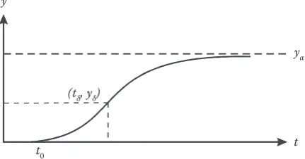
(ii) the coordinates (t_δ, y_δ) of the inflection point, when the second derivative of y with respect to t is zero, will be obtained from Eq. (2) (not including

a > 0 and b > 1) (Schnute 1981);

(iii) the curve crosses a point of the horizontal axis or the vertical one.

Eq. (2) possesses different curve shapes (e.g. S-shaped and concave shaped curves) depending on the values of a and b. Furthermore, when fitting Eq. (2) for a given data set, one does not need to subjectively place any constraint on model forms such as S-shaped or concave-shaped curves a priori. The equation can automatically fit a curve shape for a given data set and thus avoids this drawback. Therefore, this equation is able to determine whether a data set represents a growth process that shows an S-shape or a concave shape, and thus is devoid of the

a priori shape restraint.

For example, when a > 0 and 0 < b < 1, Eq. (2) demonstrates an S-shaped curve with an upper asymptote, an inflection point (t_δ, y_δ) and a time axis intersection point at age t₀. The curve is presented in Fig. 1a. This case is very common in biology and forest growth modelling (e.g. Pienaar, Turnbull 1973).

When a > 0 and b < 0, Eq. (2) shows an S-shaped curve again. Unlike in the previous case, however, the curve (see Fig. 1b) has a lower asymptote with t_{0, in addition to an upper asymptote and an} inflec-tion point (t_δ, y_δ).

These two types of curves start at a fixed point ((t₀, 0) or (0, y₀)) and increase their instantaneous growth rates monotonically to an inflection point; after this, the growth rates decrease to some final asymptotic value as determined by the genetic nature of the living organism and the carrying capacity of the environment.

When a > 0 and b > 1, Eq. (2) possesses an up-per asymptote and crosses the time axis, but has no inflection point (t_δ, y_δ). Actually, such a curve has been used widely to estimate the height-diam-eter relationship (Huang et al. 1992; Fang, Bailey 1999). This curve (Fig. 1c) shows an initial period of rapid growth and then the instantaneous growth rate monotonically decreases to some final asymptotic value.

When a < 0 and b > 1, Eq. (2) does not possess an asymptote, but it has an inflection point (t_δ, y_δ) and it intersects the t-axis at age t₀ (Fig. 1d). The curve has an initial period of decelerating growth and, passed the inflection point, continues with an indefinite period of accelerating growth. Such a curve might not occur very often in forest growth modelling. It occurs only when competition mortality leads

thinned stands to an accelerated growth in mean dbh (Bredenkamp, Gregoire 1988). This case describes unlimited growth as the independent vari-able increases and may not be strictly true as every site has a maximum capacity to support vegetation. Thus, it is not suitable for describing the long-term forest growth relationships.

When letting a > 0 and b = –1 in Eq. (2), Eq. (2) pro-duces the performance of the logistic model, which

y

y_α

(t_δ, y_δ)

t t₀

y

y_α

(t_δ, y_δ)

t t₀

y

y_α

t t₀

y

(t_δ, y_δ)

t t₀

[image:3.595.308.524.60.173.2] [image:3.595.306.523.207.327.2]

Fig. 1d. Equation (2) curve with a < 0 and b > 1 Fig. 1a. Equation (2) curve with a > 0 and 0 < b < 1

[image:3.595.307.525.489.601.2]

Fig. 1b. Equation (2) curve with a > 0 and b < 0

possesses an asymptote value and inflection point. Similarly when a > 0 and b = 1 in Eq. (2), the Eq. (2) displays the monomolecular model property which has an asymptote value but without inflection point (Lei 1998). Besides possessing the features of flexibil-ity and versatilflexibil-ity, Eq. (2) also has reasonable biologi-cal interpretations of the four estimated parameters. Parameter a is a growth rate related parameter. Pa-rameter b is a shape parameter. Parameters y₁ and y₂

can be stand (or tree) ranges corresponding to initial and final values of the dependent variables for a given single observation data set, respectively (if a data set is a pooled data set, y₁ and y₂ can be mean values of dependent populations with the beginning age (t₁) and the end age (t₂)). Therefore, y₁ and y₂ can be considered as indicators of stand or forest structure (Fang, Bailey 1999).

MATERIALS AND METHODS

The flexibility and versatility of Eq. (2) were dis-cussed and analyzed from a statistical point of view. Four different data sets were used with Eq. (2) to demonstrate this feature of discerning functional forms.

Dataset 1 for stand dominant height vs. stand age

Remeasurement data from a Eucalyptus globulus

Labill. forest inventory collected by the SILVICAIMA company in Portugal in 1990–1995 were used (Lei 1998), from which a total of 169 plots from 11 lo- cations were taken for this study. The sample plots contained repeated measurements: 90 plots were measured twice, 49 plots were measured three times and 30 plots were measured four times (Table 1). 447 observations were produced from the 169 plots at the stand level.

Dataset 2 for tree height-diameter

The data set consists of 9 Japanese fir trees stem analysis data from 4 plots in the Experimental Forest College of Agriculture, National Taiwan University (Zeide 1999). 280 observations were made on the 9 trees (Table 1).

Dataset 3 for tree dbh vs. tree age

The eucalypt tree dbh growth data set from FAO Forest Series (1979) is used and Table 1 describes the statistics of the data set.

Data 4 for tree height vs. tree age

The mean tree height values in decimetres for ages 2–19 are employed and Table 1 demonstrates the statistics of this data set.

These data sets are selected for the analysis because they represent different growth curve shapes. Eq. (2) can be used to fit the data sets in different ranges of parameters. For discernment and comparison pur-poses, the Meyer function (1940) with three and two parameters, h = a + b(1 – e–ct_{), was also employed,}

because this function has been used extensively in the height-diameter relationship and recommended as an appropriate model to describe the relationship. The Meyer function, however, is only able to describe a concave curve and does not have the flexibility and versatility of the Schnute model. Therefore, it cannot discern different functional shapes for different data sets. The models were evaluated using residual mean squared error (RMSE), mathematical properties and the biological interpretations of model parameters.

All the results presented were computed using the non-linear JMP Software program (SAS Institute Inc. 1994). The Gauss-Newton method of using the Taylor series linearization (Neter et al. 1985) was applied, and multiple starting values were provided for the parameters to ensure that the least squares solution was based on a global, rather than on a lo-cal, minimum.

RESULTS AND DISCUSSION

Case 1: SILVICAIMA data set for stand dominant height vs. stand age (a > 0 and b < 0)

[image:4.595.65.536.73.163.2]

As shown in Fig. 5, the scatterplot of stand domi-nant height vs. stand age did not indicate a specific functional form. It is difficult to determine the functional form based on this plotting. As suggested previously, Eq. (2) was used first to determine the functional form. The result suggests an S-shape

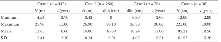
Table 1. Statistics of the different data sets

Case 1 (n = 447) Case 2 (n = 280) Case 3 (n = 76) Case 4 (n = 36)

H (m) t (year) H (m) dbh (cm) dbh (cm) t (year) H (cm) t (year)

Minimum 4.54 2.70 0.42 0 6.30 2.00 12.00 2.00

Maximum 25.90 11.00 26.90 30.10 26.50 20.00 221.00 19.00 Mean 13.85 6.60 16.06 16.69 18.24 11.00 85.21 10.50

S.D. 5.41 2.30 8.24 8.91 4.65 5.51 61.53 5.26

form due to a = 0.9557 (> 0) and b = –5.547 (< 0) for the given data set. The results are listed in Table 2 and the estimated curve is shown in Fig. 2. Then, a model pool of S-shapes can be collected for selec-tion and comparison to get the “best” model on the basis of some criteria: ease of convergence, biological interpretation of parameters, the asymptotic t -sta-tistics of the parameters and mean squared error (MSE) of the models. Here the Meyer function was used with the three parameters to estimate the data set as well, but it failed to converge. The model

[image:5.595.64.536.72.250.2]

h = b(1 – e–ct_{) was also used to fit the data (Table 2).}

Table 2 and Fig. 2 suggest that the S-shape curve can fit the given data set better than the concave curve because RMSE in Eq. (2) (3.0057) is smaller than that of the Meyer model (3.0338). In addition

the biological interpretations of Eq. (2) parameters (see Section 2) are more reasonable than those of the Meyer model. The asymptote (A) and the inflection point (t_δ, H_{δ for Eq. (2) are:}

_Hb

2 – Hb1

A =

[

Hb

1 +

]

1/b

= 21.83 m 1 – e–a(t2 – t1)

1 b(ea × t_2Hb

2 – ea × t1Hb1)

t_δ = t₁ + t₂– ln

[

]

= a Hb2 – Hb1

= 9.07 years

(1 – b)(ea × t_2Hb

2 – ea × t1Hb1)

H_δ =

[ ]

1/b= 15.55 m (ea × t2 – ea × t1)

where the A appears reasonable, given the ranges of the observed data. The A is also similar to those estimated by Amaro et al. (1998) and Tome et al. (1995). For the Meyer function, the asymptote (A) is 79.95 m that is quite different from Eq. (2)’s, and the inflection point does not exist. In summary, the pre-sented example suggests that a pool of models with an S-shape would be more suitable for describing (or fitting) the given data set than that with a concave shape or an S-shape and concave shape.

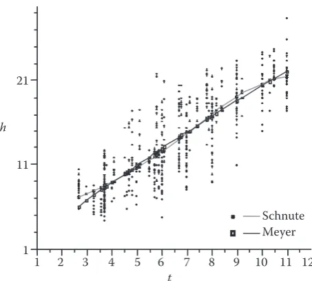
Case 2: Japanese fir data set for height-diameter (a > 0 and 0 < b < 1)

From the observations, it can be seen that arbitrary restraint (0, 1.3) on a data pair (dbh, height) may not be suitable for the data set. As shown in Fig. 3, the curve shape of the height-diameter relationship for this species can be regarded as either concave or sigmoid. As in the previous case, Eq. (2) was used first to determine the type of curve shape. The results are listed in Table 2 and the fitted curve is shown in Fig. 3. The curve for the height-diameter

relation-Table 2. Parameter estimates for the Schnute and Meyer models using different data sets (or cases)

Function Parameter Case 1 Case 2 Case 3 Case 4

Eq. (2)

a 0.9557 0.0491 0.1046 –0.03187

b –5.547 0.5093 1.8284 2.3422

y₁ 5.345 1.654 5.141 11.263

y₂ 19.479 20.102 21.542 217.290

A 21.83 29.35 23.43 n.a.

t_δ 9.07 8.39 n.a. 4.09

y_δ 15.55 7.25 n.a. 24.07

RMSE 3.0057 1.9794 1.0377 3.1055

Meyer model

b 79.9563 170.3671 23.3564 n.a.

c 0.0295 0.0059 0.1768 n.a.

RMSE 3.0338 1.9992 1.0682 n.a.

n.a. – not available, a, b, c – parameters of Schnute and Meyer models, respectively, RMSE – root mean squared error of estimation, A – asymptote, t_δ, _yδ – the coordinates of the inflection point

h

Schnute Meyer 1

11 21

1 2 3 4 5 6 7 8 9 10 11 12

t

Schnutee

Meyer

1 2 3 4 5 6 7 8 9 10 11 12e

t h

11

1 21

[image:5.595.311.523.340.480.2] [image:5.595.64.291.509.713.2]

ship is sigmoid. The Meyer function with the three parameters was used to fit the data set as well, but it could not achieve convergence (surprisingly, it could not be achieved even if different values were given to parameter a, using nonlinear regression to fit b and

c in the two parameter-Meyer function). Though

h = b(1 – e–c(dbh)_{) can attain convergence for the data} set and appears a concave curve, this model cannot explain the height-diameter relationship reasonably. For example, the model gives a zero height when dbh = 0. This does not reflect the realistic relation-ship of height-diameter from the data set. In fact h is greater than zero when dbh = 0 (Table 1). However, Eq. (2) can meet the requirement. From Table 2, the residual mean squared errors are almost the same between the Meyer model (1.9992) and the Schnute model (1.9794), whereas the shapes of the two curves described in the two models are different at both up-per and lower points. The upup-per and the lower ends of both curves apparently show different values of the two models. The Meyer model has a lower value than the Schnute model at the lower end of the solid line, while it has a higher value than the latter at the up-per end of the line. The asymptote values (A) for Eq. (2) and the Meyer model are 29.35 and 170.37 me- ters, respectively. The asymptote value of the Meyer model is in excess of the dominant height value 30 meters (Guan pers. commun.), indicating that the asymptote parameter of the model has no biological significance. Eq. (2) possesses the inflection point (t_δ = 8.39 cm, H_δ=7.25 m), while the Meyer model lacks an inflection point. In terms of the mathemati-cal and biologimathemati-cal properties of the models, Eq. (2) is obviously better than the Meyer model in this case

though the statistical criteria of the two models are basically equivalent. The results of this case also suggest that a model of pool with S-curve shapes rather than concave-curve shapes be considered as candidate models for the purpose of comparison and selection.

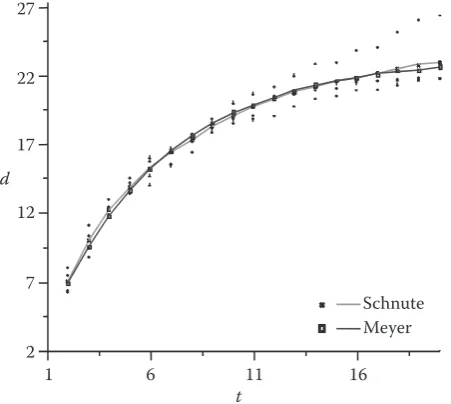
Case 3: Eucalypt tree dbh (cm) vs. tree age (a > 0 and b > 1)

The estimated parameters of Eq. (2) and of the Meyer function are listed in Table 2 and the fitted curve is depicted in Fig. 4. The asymptotes (A) in Eq. (2) and the Meyer model are

dbhb

2 –dbhb1 23.43

(

A =

[

dbhb

1 +

]

1/b

)

1 – e–a(t2 – t1)

and 23.36 cm, respectively. RMSEs of Eq. (2) and the Meyer model are 1.0377 and 1.0482, respectively. The results show that the data set is a concave shape with no inflection point, and both functions are suit-able for this data set because they basically give the similar results in statistical criteria, mathematical properties and biological interpretations and curve shape as well. This case suggests that a model pool of concave shapes rather than S-shape curves be collected for comparison and selection in the given data set.

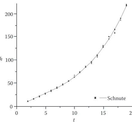
Case 4: A case where neither Bertalanffy-Richards nor Meyer functions are suitable (a < 0 and b > 1)

Dataset 4 is employed because the type of data in case 4 is very difficult to be obtained in order to further demonstrate the flexibility and versatility of the Schnute model in comparing and selecting growth models under the conditions of a < 0 and

b > 1. Eq. (2) was used to estimate the growth curve 0

5 10 15 20 25 30

0 5 10 15 20 25 30

d h

Schnute Meyer

Schnutee

Meyer

d h

10

0 25

0 5 10 15 20 25 30e

30

20

15

[image:6.595.63.286.57.262.2]

5

Fig. 3. A comparison of estimated heights of Japanese fir, ana-lyzed with the Schnute and the Meyer models

2 7 12 17 22 27

1 6 11 16

t d

Schnute Meyer

27

7 12 17

d

22

2

Schnute Meyer

1 6 11 16

[image:6.595.312.538.59.261.2]

t

for the given data set. The estimated results are listed in Table 2 and the fitted curve is presented in Fig. 5. As previously discussed, Eq. (2) in the condition of

a < 0 and b >1 only has the inflection point (t_δ, H_δ) as follows:

1 b(ea × t_2Hb

2 – ea × t1Hb1

t_δ = t₁ + t₂ – ln

[

]

= 4.09 years a Hb2 – Hb1

(1–b)(ea × t_2Hb

2 – ea × t1Hb1

H_δ =

[ ]

= 24.07 cm (ea × t2 – ea × t1)

As shown in Fig. 5, Eq. (2) can fit the given data set very well. However, the Meyer function, includ-ing either 2 or 3 parameters, failed to fit the data set because the function can describe only the concave shape curve and does not possess the properties of flexibility and versatility. Though the Bertalanffy-Ri-chards function possesses features similar to those of the Schnute function, the former is not suitable for describing the data set (Lei et al. 2001). However, the derived form (3) (e.g. m < 0 and r < 0) of the Berta-lanffy-Richards function can fit the data set:

y = A’ [B’ exp(k’t – 1)]1/(1 – m) ₍₃₎ where Eq. (3) is derived from

dy

= ηym – ry dt

(Richards 1959) when m < 0 and r < 0 (let r’ = – r). The parameter relationships between Eq. (3) and Eq. (2) can be written:

a = –r’ (1 – m) = – k’

b = 1 – m

A´= [yb

2/B´(eat2 – 1)]1/b

B´= [ea(t_{2 +} t_{1) × (y}b

2 – yb1)] / [eat2 × yb2 – eat1 × yb1]1/b (4)

CONCLUSIONS

Three functional forms including sigmoid, concave and parabolic curves were used to describe forest growth processes and the height-diameter relation-ship. As indicated before, the traditional method has drawbacks in the model comparison and selection process. The model forms with different mathemati-cal properties are subjectively constrained a priori to the analyzed data set, and consequently a consider-able bias may arise for some models. Some of the models may not be able to achieve convergence at all. In addition, a considerable amount of time is needed for the process of the model comparison and selec-tion. The process of the real data analysis estimation described in this paper suggested that using the Schnute model could overcome those drawbacks and thus is more effective in selecting the “best” model from candidate models because the Schnute model has enough flexibility and versatility to efficiently determine the curve shape suitable for different data sets. Furthermore, the biological interpretation of the model parameters is reasonable. The model is also easier to fit and quicker to achieve convergence regardless of the data set. With the current method, no suitable functional form for a given data set is known before the selection process. Therefore, it is recommended that the Schnute model be used as the first step to determine the appropriate func-tional form in order to avoid assuming a curve shape

a priori.

Acknowledgements

The authors would like to thank Dr. Boris Zeide, Department of Forest Resources, University of Ar-kansas in Monticello, USA, for providing his data to this study.

References

AMARO A., REED D., TOMÉ M., THEMIDO I., 1998. Mod-elling dominant height growth: eucalyptus plantations in Portugal. Forest Science, 44: 37–46.

BREDENKAMP B.V., GREGOIRE T.G., 1988. A forestry ap-plication of Schnute’s generalized growth function. Forest Science, 34: 790–797.

CIESZEWSKI C.J., 2001. Three methods of deriving advanced dynamic site equations demonstrated on inland Douglas-fir site curves. Canadian Journal of Forest Research, 31: 165–173.

0 50 100 150 200

0 5 10 15 20

t h

Schnute

200

h

Schnute

0 5 10 15 20

t

50 100 150

[image:7.595.69.290.51.254.2]

0

CIESZEWSKI C.J., BELLA I.E., 1992. Towards optimal de-sign of nonlinear regression models. In: RENNOLLS K., GERTNER G., Proceedings of a IUFRO S4.11 Conference held on 10–14 September 1991 at the University of Green-wich, London.

CIESZEWSKI C.J., BELLA I.E., 1993. Modelling density-related lodgepole pine height growth, using Czarnowskis stand dynamics theory. Canadian Journal of Forest Re-search, 23: 2499–2506.

CIESZEWSKI C.J., BAILEY R.L., 2000. Generalized algebraic difference approach: theory based derivation of dynamic site equations with polymorphism and variable asymptotes. Forest Science, 46: 116–126.

CLUTTER J.L., FORTSON J.C., PIENAAR L.V., BRISTER G.H., BAILEY R.L., 1983. Timber Management: a Quantita-tive Approach. New York, John Wiley and Sons: 333. FANG Z., BAILEY R.L., 1999. Height-diameter models for

tropical forest on Hainan Island in southern China. Forest Ecology and Management, 110: 315–327.

FAO Forest Series, 1979. Eucalyptus for planting. Rome, FAO: 667.

HUANG S., TITUS S.J., WIENS D.P., 1992. Comparison of nonlinear height-diameter functions for major Alberta tree species. Canadian Journal of Forest Research, 22: 1297–1304.

LEI Y.C., 1998. Modelling forest growth and yield of Euca-lyptus globulus Labill. in Central-interior Portugal. [Ph.D. Thesis.] UTAD, Vila Real, Portugal: 155.

LEI Y.C., MARQUES C.P., BENTO J.M., 2001. Features and applications of Bertalanffy-Richards’ and Schnute’s

growth equations. National Resource Modeling, 14: 433–451.

MEYER H.A., 1940. A mathematical expression for height curves. Journal of Forestry, 38: 415–420.

NETER J., WASSERMAN W., KUTNER M.H., 1985. Applied Linear Regression Mode. USA, IRWIN.

PENG C.H., ZHANG L., LIU J., 2001. Developing and validat-ing nonlinear height-diameter models for major tree species of Ontario’s boreal forests. Northern Journal of Applied Forestry, 18: 87–94.

PIENAAR L.V., TURNBULL K.J., 1973. The Chapman-Ri-chards generation of von Bertalanffy’s growth model for basal area growth and yield in even-aged stands. Forest Science, 19: 2–22.

RICHARDS J., 1959. A flexible growth function for empirical use. Journal of Experimental Botany, 10: 290–300. SAS Institute Inc., 1994. User’s Guide for JMP Statistic,

Ver-sion 3. NY, Cary.

SCHNUTE J., 1981. A versatile growth model with statisti-cally stable parameters. Canadian Journal of Fisheries and Aquatic Sciences, 38: 1128–1140.

THOMPSON D.A., BONNER J.T., GOULD S.J., 1992. On Growth and Form. Cambridge, Cambridge University Press: 368.

TOME M., FALCÃO A., CARVALHO A., AMARO A., 1995. A global growth model for eucalypt plantations in Portugal. Lesnictví-Forestry, 41: 197–205.

Received for publication October 22, 2005 Accepted after corrections November 1, 2005

Srovnání a výběr růstových modelů s použitím Schnuteho modelu

Y. Lei1_{, S. Y. Zhang}2

1_{Research Institute of Forest Resource Information and Techniques, Chinese Academy of Forestry,}

Beijing, China

2_{Resource Assessment and Utilization Group, Quebec, Canada}

Corresponding author:

Dr. Yuancai Lei, Research Institute of Forest Resource Information and Techniques, Chinese Academy of Forestry, Beijing 100091, P. R. of China

tel.: + 010 628 891 99, fax: + 010 628 883 15, e-mail: [email protected], [email protected]

ukazují, že model má vhodné vlastnosti, takže výsledná křivka může mít tvar sigmoidní, konkávní či jiný. Vzhledem k tomu, že předem není znám vhodný tvar křivky pro daný soubor dat, je vhodné použít nejdříve Schnuteho model,

díky kterému zjistíme tvar vhodné křivky a vyhneme se tak nutnosti volby vhodného modelu a priori.