Evaluation of Causal Discovery Models in
Bivariate Case Using Real World Data
Jing Song, Satoshi Oyama, Haruhiko Sato, and Masahito Kurihara
Abstract—Causal relationships are different from statistical relationships. Distinguishing cause from effect is a fundamental scientific problem that has attracted the interest of many researchers. Among causal discovery problems, discovering bivariate causal relationships is a special case because the well-known independent tests are useless. We empirically tested three existing state-of-the-art models, ANM, PNL model, and IGCI model, for causal discovery in the bivariate case using real world data and compared their performance using three metrics: accuracy, area under ROC curve (AUC), and time cost to make a decision. We concluded the strong points and weaknesses of each method through our experiments. For the efficiency of algorithm, we found that the IGCI model is the fastest even when the dataset is large and that the PNL model costs the most time to give a decision.
Index Terms—causal discovery, bivariate, accuracy, area under curve, time cost.
I. INTRODUCTION
People are generally more concerned with causal rela-tionships between variables than they are with statistical relationships between variables, and “causality” [1], [2], [3], [4] has attracted the interest of researchers in various fields, including economics, sociology, and machine learning. The best way to verify causal relationship between variables is to conduct a controlled experiment. However, in the real world, such experiments are often too expensive, unethi-cal, or even impossible. Many researchers are thus using statistical methods to analyze causal relationships between variables [5], [6], [7], [8]. Some concepts of causality have been formalized using directed acyclic graphs. As a general algorithm for causal discovery, a conditional independence test can be used to exclude irrelevant relationships between variables [3], [4]. However, in the case of two variables, a conditional independence test is impossible. Several models have been proposed to solve this problem [9], [10], [11], [12], [13], [14], [15].
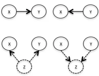
For two variables X and Y, there are four possible re-lationships, besides independence and feedback, between them (Figure 1). The top two diagrams in Figure 1 show the possible causal relationships between X and Y. The remaining task is to decide the direction of the arrow. The bottom two diagrams represent the “common cause” (left) and “selection bias” (right) case. The unobserved variables Z are “confounders”1 for causal discovery between X and Y. The existing of “confounders”2 will bring spurious cor-relation between X and Y. How to distinguish spurious
The authors are in the Division of Computer Science and In-formation Technology in the Graduate School of InIn-formation Sci-ence and Technology, Hokkaido University, Sapporo, Japan, 060-0814. Email:[email protected], [email protected], [email protected], [email protected]
[image:1.595.340.511.176.308.2]1For the definition of confouding, please refer to [16], [17]. 2The number of “confounders” is not limited to one.
Fig. 1. Four Possible Relationships between X and Y (Besides Indepen-dence and Feedback).
correlation with “confounders” from actual causality is a remaining challenging task in this field. Many current models are based on the assumption that “confounders” do not exist.3 We compared the performance of three existing state-of-the-art models, ANM, PNL and IGCI, under the assumption that confounders do not exist. We used three metrics: accuracy, area under ROC curve (AUC), and time cost to make a decision.
In section II, we introduce some related work in causal discovery. In section III, we briefly introduce the three models: ANM, PNL and IGCI. In section IV, we describe the dataset we used and the implementation of the three models. In section V, we present the results and give a detailed analysis of the performance of the three models. We conclude in section VI by summarizing the advantages and weaknesses of the three models and mentioning future tasks.
II. RELATEDWORK
Granger causality [6] is proposed to detect causal direction of time series data based on temporal ordering of variables. Granger causality only works on the linear stochastic sys-tems. Chen et al. [21] extends the model to work on nonlinear systems. For Granger causality [6] and extended Granger causality [21], temporal information is needed.
Shimizu et al. [18] proposed the LiNGAM (short for linear non-gaussian acyclic model) which can detect causal direc-tion of varialbes no matter whether temporal informadirec-tion is available or not. The LiNGAM works when the causal relationship between variables is linear, the distributions of disturbance variables are non-Gaussian and the network structure can be expressed using DAG (short for directed
3Dealing with confounders is an on-going work in this field. As far as we
acyclic graph). Some extensions of LiNGAM has been proposed [22], [19], [23], [20].
LiNGAM is based on the assumption of linear relation-ships between variables. Hoyer et al. [12] propose additive-noise model (ANM) to deal with non-linear relationships. When the regression function is linear, ANM works in the same way as LiNGAM. Zhang et al. propose the post non-linear (PNL) model which takes into account the nonnon-linear effect of causes, additive inner noise and external sensor distortion. A brief introduction of ANM and PNL will be given in section III.
The above methods are based on the structural equation modeling (SEM) which requires structural constraints on the data generating process. Another research direction is based on the assumption of independent mechanisms of nature to generate causes and effects. The idea is that the shortest description of joint distribution p(cause, ef f ect)
can be expressed by p(cause)p(ef f ect|cause). Compared withp(ef f ect)p(cause|ef f ect),p(cause)p(ef f ect|cause)
has lower total complexity.
Janzing et al. [14], [15] propose information geometric causal inference (IGCI) model to infer asymmetry between cause and effect through the complexity loss of distributions. A brief introduction of IGCI will be given in the following section. Zhang et al. [24] propose a bootstrap-based approach to detect causal direction based on the condition that the parameters of the cause involved in the causality data gen-erating process is exogenous from that of the cause to the effect. Mooij et al. [11] propose a probabilistic latent variable model (GPI) to distinguish between cause and effect using standard Bayesian model selection.
In the above work, accuracy is usually used to evaluate the performance of causal discovery models. Besides of accuracy, we use an evaluation method for a binary classifier: area under ROC curve (AUC) as another evaluation method in our work. We compare existing methods using three metrics: accuracy, AUC, and time cost to make a decision.
III. MODELS
The three models we choose in our experiments were the additive-noise model (ANM) [12], the post non-linear (PNL) model [13], [25], and the information geometric causal inference (IGCI) model [14], [15]. The three models are typical and state-of-the-art models for causal discovery in bivariate case. The first two models define how causality data is generated in nature. The last model finds the asymmetry between cause and effect through the complexity loss of distributions.
A. ANM
The additive noise model (ANM) of Hoyer et al. [12] is based on two assumptions: the observed effects can be expressed using functional models of the cause and additive noise (Equation 1) and the cause and additive noise are independent. If f()is a linear function and the noise has a non-Gaussian distribution, ANM works in the same way as the linear non-Gaussian acyclic model (LiNGAM) [18]. The model is learned by performing regression in both directions and calculating the independence between the assumed cause and noise (residuals) for each direction. The decision rule
is to choose the direction with the larger independence as the true causal direction. ANM cannot deal with the linear Gaussian case since the data can fit the model in both directions, so the asymmetry between cause and effect disappears. In [26], Gretton et al. improved the algorithm and extended ANM to work even in the linear Gaussian case [26]. The improved model also works more efficiently in the multivariate case.
ef f ect=f(cause) +noise (1)
B. PNL Model
In the post-nonlinear (PNL) model of Zhang et al. [13], [25], effects are nonlinear transformations of causes with some inner additive noise, followed by an external nonlinear distortion (Equation 2). From Equation 2, we can get that noise=f2−1(ef f ect)−f1(cause), where cause and effect
are the two observed variables. To identify the cause and effect, nonlinear independent component analysis (ICA) is performed to extract two components that are as independent as possible. The extracted components should be independent for the true direction. The validity of the PNL model has been proven [25].
ef f ect=f2(f1(cause) +noise) (2)
C. IGCI Model
The IGCI model [14], [15] is based on the hypothesis that if “X causes Y,” the marginal distribution p(x) and the conditional distribution p(y|x) are independent. The IGCI model gives an information-theoretic view of additive noise and defines independence by using orthogonality. With the ANM [12], if there is no additive noise, inference is impossible while it is possible with the IGCI model.
The IGCI model determines the causal direction on the basis of complexity loss. Let νx and νy be the reference distributions for X and Y.D(Px||νx) :=
R
logPν(x) (x)P(x)dx is the KL-distance between Px and νy, which works as a feature of the complexity of the distribution. The complexity loss from X to Y can be defined by
VX→Y :=D(Px||νx)−D(Py||νy). (3) The decision rule of the IGCI model is that, ifVX→Y <0, infer “X causes Y,” else ifVX→Y >0 infer “Y causes X.” This rule is rather theoretical. An applicable and explicit form for the reference measure is entropy-based IGCI or slope-based IGCI.
1) Entropy-based IGCI:
ˆ
S(PX) :=ψ(m)−ψ(1) + 1
m−1
m−1 X
i=1
log|xi+1−xi|
(4)
ˆ
VX→Y := ˆS(PY)−Sˆ(PX) =−VYˆ →X (5) 2) Slope-based IGCI:
ˆ
VX→Y :=
1
m−1
m−1 X
i=1
log
yi+1−yi xi+1−xi
The explicit form of IGCI is simpler, and we can see that the two IGCI models coincide with each other. The calculation does not cost much time even when dealing with big data. However, the IGCI model prefers low-noise data and may perform poorly in a high-noise situation. We discuss the strengths and weaknesses of the IGCI model in section V.
IV. EXPERIMENTS
In this section, we describe the data used in our experi-ments and the implementation of each model. The results are presented in section V.
A. Dataset
We used the CauseEffectPairs (CEP) [27] dataset, which contains 97 pairs of real world causal variables with the gold standard labeled for each pair. The data set is publicly available online [27]. Some of the data were collected from the UCI Machine Learning Repository [28]. The data comes from various fields, including geography, biology, physics, and economics. The dataset also contains time series data. Most of the data contains much noise. An appendix contains a detailed description of each pair of variables [29].
We used 91 of the pairs in our experiments since some of the data (e.g, pair0052) in CEP [27] contains multi-dimentional variables4. Scatter plots of the data are shown in Figure 2. The variables range in size from 126 to 16,382. The variety of data types makes causal analysis using real world data challenging. Moreover, the dataset is not well balanced: of the 91 pairs, the true label is “X causes Y” for 67 pairs and “Y causes X” for the other 24 pairs.
B. Implementation Details
We implemented the three models as described in the original work.
a) ANM: Using the reported experiment settings [12], we performed Gaussian processes for machine learning regression [30], [31]. We then used the Hilbert-Schmidt Independence Criterion (HSIC) [32] to test the independence between the assumed cause and residuals. The dataset used had been labeled with the true causal direction for each pair with no independence, or feedback. Using the decision rule of ANM, we determined that the direction with the greater independence was the true causal direction.
b) PNL: We used nonlinear ICA to extract the two components that were assumed to be the cause and noise if the model had been learned in the right direction. The nonlinearities off1andf2−1in Equation 2 were modeled by
multi-layer perceptrons. By minimizing the mutual informa-tion between the two output components, we made the output as independent as possible. After extracting two independent components, we tested their independence by using HSIC [32]. Finally, in the same way as for ANM, we determined that the direction with the greater independence was the true one.
4The three models we implemented in our experiment cannot deal with
[image:3.595.312.541.49.360.2]multi-dimentional data.
Fig. 2. Scatter Plot of Data Used in Experiments
c) IGCI(entropy,uniform): Compared with the other two models, the implementation of the IGCI model is sim-pler. We used reported equations (4, 5) to calculate VˆX→Y and VˆY→X and determined that the direction in which entropy decreased was the true direction. If VˆX→Y < 0, the inferred causal direction was “X causes Y”; otherwise, it was “Y causes X.” For the IGCI model, the data should be normalized before calculating VXˆ →Y and VYˆ →X. In accordance with the reported experiment results, we used the uniform distribution as the reference distribution because of its good performance. For the repetitive data in the dataset, we setlog0 = 0.
d) IGCI(slope,uniform): The implementation of the IGCI(slope, uniform) model was similar to that of the IGCI(entropy, uniform) one. We used (6) to calculateVˆX→Y andVˆY→X and determined that the direction with a negative value was the true one. For the same reason as above, we mapped the data to [0,1] before calculatingVXˆ →Y and
ˆ
VY→X. To make (6) meaningful, we filtered out the repetitive data.
V. RESULTS
Since causal discovery models in the bivariate case give a decision between two choices, we can regard these models as binary classifiers and evaluate them using the area under ROC curve (AUC). Although there is difference between the outputs of the three models and a binary classifier, we propose a way to overcome this problem. It is described in subsection V-B.
Finally, we compare model efficiency by calculating the average time needed to give a decision. This is described in subsection V-C.
A. Accuracy For Different Decision Rates
We calculated the accuracy of each model for different decision rates using (7) and (8) and plotted the results (Figure 3). The decision rate changed when the threshold was changed. The larger the threshold, the more stringent the decision rule. In an ideal situation, accuracy decreases as the decision rate increases, with the starting point at 1.0. However, the results with real world data were not perfect because there was much noise in the data.
As shown in Figure 3, the accuracy started from 1.0 for the ANM and IGCI model and from 0.0 for the PNL model. This means that the PNL model gave the wrong decision when it had the highest confidence. Investigation showed that PNL model made a wrong decision with the highest confidence because of the discretization of data5. Besides, we can see that, although the accuracy of the IGCI model started from 1.0, the accuracy dropped sharply when the decision rate was between 0.0 and 0.2. The reason why accuracy drops is that IGCI made wrong decisions with large confidence when dealing with pair0056-pair0063. These eight pairs of variables contain much noise which makes IGCI give bad performance. Besides, there are some “outliers” for the eight pairs which affect the decision result much6. After reaching a minimum, the accuracy increased continuously and became more stable. Compared with the other models, the accuracy of ANM was relatively stable with a starting value of 1.0. When all decisions have been made, the accuracies of these models are ranked IGCI > AN M > P N L.
DecisionRate:= NDecision
NData
(7)
Accuracy:= NT rueDecision
NDecision
(8)
B. Area Under ROC Curve (AUC)
Besides calculating the accuracy of the three models for different decision rates, we used the area under ROC curve (AUC) to evaluate their performance.
As described in IV-A, the dataset is not well balanced. Although the three models did not train a classifier from the data, the inference method can be seen as a binary classifier. For a binary classifier, a well- known evaluation method is the area under ROC curve (AUC). The ROC curve is plotted
5PNL makes wrong decision with the largest confidence when dealing
with pair0070 in [27]. One variable of pair0070 contains only two values: 0 and 1. The variable is easy to be inferred as the cause according to the mechanism of PNL model.
6This is because that the calculation methods of IGCI (Equation 4,5,6) is
[image:4.595.326.535.60.217.2]susceptible to “outliers”.
Fig. 3. Accuracy of Three Models for Different Decision Rates.
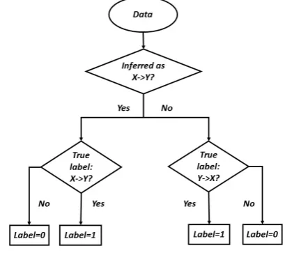
Fig. 4. Process to Label Every Pair of Variables.
by calculating the true positive rate (TPR) and false positive rate (FPR) for different thresholds. The output of a binary classifier is a value in the interval [0,1]. In contrast, for the three models evaluated here, the outputs were the two values calculated for the two possible causal directions. Despite this difference, we used the following steps to get the ROC curve and at the same time not break the decision rule of the three models.
1) Divide the data into two groups: a) inferred as “X causes Y” and b) inferred as “Y causes X” in accor-dance with the decision rule of the model.
2) LetVX−>Y andVY−>X be the outputs of the models. Calculate the absolute value of the difference between VX−>Y and VY−>X (Equation 9) and map Vdif to [0,1].
3) Label every pair of data in accordance with the process diagrammed in Figure 4.
4) UseVdif and the generated labels in 1) to calculate the TPR and FPR for different thresholds. Plot the ROC curve and calculate the corresponding AUC value.
[image:4.595.322.527.259.442.2]basic rule of causal discovery models needs to be observed. For example, we cannot use the division of VX−>Y and VY−>X in the same way as the output of a binary classifier. If we did, the decision rule of the models would be broken if the threshold was set very large or small. However, if we divide the data into two groups in accordance with the decision result, we not only take into consideration different levels of punishment but also observe the original decision rule.
In step 2), we used the absolute value of the difference between VX−>Y and VY−>X as the “confidence” of the model when giving a decision. The larger the Vdif, the greater the confidence. We did not use division because, if one of VX−>Y and VY−>X was very small, the division result would be very large. We mapped Vdif to [0,1] to make the calculation more convenient. In this way, Vdif could be used in the same way as the output of a binary classifier. For causal discovery, the larger theVdif, the greater the confidence in the decision. At the same time, more punishment should be given when the decision is wrong.
In step 3), we labeled the data in accordance with the diagram in Figure 4. For the decision “X causes Y,” the positive class was “X causes Y.” We checked the dataset to see whether the true label was “X causes Y.” If it was, the data was labeled as a positive class, otherwise it was labeled as a negative class. The same process was done with the decision “Y causes X”; however, the label was opposite since in this group “Y causes X” is the positive class.
In step 4), we used the normalizedVdif as the confidence of a decision and the label assigned in step 3) to calculate TPR and FPR for different thresholds. We plotted TPR and FPR to get the ROC curve and calculated the corresponding AUC value.
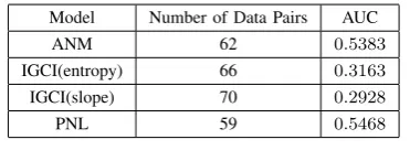
The results are plotted in Figures 5 and 6. The corre-sponding data sizes and AUC values are shown in Tables I and II. The IGCI model performed poorly when it gave “X causes Y.” The AUC values for the IGCI model when the decision was “X causes Y” were smaller than 0.5, which means its performance was even worse than that of a random classifier. However, as described in subsection V-A, when we used different decision rates, the IGCI model had the best performance.
[image:5.595.334.520.528.601.2]We checked the decisions made by the IGCI model and found that it made several wrong decisions when the threshold was large. Such decisions with a large threshold are punished severely when using the area under ROC curve (AUC) metric. As shown in Figure 3, although the accuracy of the IGCI model started from 1.0, it dropped sharply when the decision rate was between 0.0 and 0.2. A wrong decision with a small decision rate was not be punished much when evaluating accuracy for different decision rates. However, for the area under ROC curve (AUC), a wrong decision when the threshold was large was punished more than when the threshold was small. For these reasons, the starting point of the ROC curve for IGCI model in Figure 5 has been shifted to the right, making AUC less than 0.5. For the decision “Y causes X,” the models performed better when evaluating with the area under ROC curve (AUC), especially the IGCI one. In this group, the IGCI(entropy) model had the largest AUC (0.7222). Compared with the other models, ANM had similar AUC values for both groups, demonstrating the stableness of
Fig. 5. ROC of Three Models When Decision was “X Causes Y.”
Fig. 6. ROC of Three Models When Decision was “Y Causes X.”
TABLE I
AUCOF THREE MODELS WHEN DECISION WAS“X CAUSES Y.”
Model Number of Data Pairs AUC
ANM 62 0.5383
IGCI(entropy) 66 0.3163
IGCI(slope) 70 0.2928
PNL 59 0.5468
TABLE II
AUCOF THREE MODELS WHEN DECISION WAS“Y CAUSES X.”
Model Number of Data Pairs AUC
ANM 29 0.5404
IGCI(entropy) 25 0.7222
IGCI(slope) 21 0.6923
PNL 32 0.6537
ANM. For the PNL model, the AUC value was larger but not as high as the one for the IGCI model.
C. Algorithm Efficiency
[image:5.595.338.516.627.690.2]TABLE III
TIME COST TO MAKE A DECISION
Model Time Cost ANM 10.7±7.4s
PNL 80.5±19.5s
IGCI(entropy) 0.0014±0.0019s
IGCI(slope) 0.0014±0.0017s
algorithm to give a decision. We performed the experiment on the MATLAB platform with an Intel Core i7-4770 3.40 GHz2 CPU and 8.00 GB memory. From Table III, we can see that the IGCI model was the most efficient one while the PNL model was the least efficient. ANM was in the middle. The high time cost of the PNL model was due to the modeling nonlinearity off2−1 andf1 in Equation 2.
VI. CONCLUSION
We compared three existing state-of-the-art models (ANM, PNL model, IGCI model) for causal discovery in the binary case with real world data. Testing using different decision rates showed that the IGCI model had the best performance. To check whether the decisions made were reasonable, we used a binary classifier metric: the area under ROC curve (AUC). The IGCI model had a small AUC value for the decision “X causes Y” because it made several wrong decisions when the threshold was high. Compared with the other models, the ANM results were relatively stable. Finally, we compared the time cost when making a decision. The IGCI model was the fastest even when the dataset was large. The PNL model cost the most time to give a decision.
Of the three models, the IGCI one had the best perfor-mance when there was little noise and the data were not discretized much. Improving the performance of the IGCI model when there is much noise and how to deal with discretized data are future tasks. Although the performance of ANM was relatively stable, overfitting should be avoided for ANM. Of the three models, the PNL model is the most generalized one as it takes into account the nonlinear effect of causes, additive inner noise, and external sensor distortion. However, modeling the nonlinearities of f1 andf2−1 takes
much time for the PNL model.
ACKNOWLEDGMENTS
This work was supported by a grant in aid from Japan Society for the Promotion of Science (15K1214805).
REFERENCES
[1] C. W. Granger, “Some recent development in a concept of causality,”
Journal of econometrics, vol. 39, no. 1, pp. 199–211, 1988. [2] J. Y. Halpern, “A modification of the halpern-pearl definition of
causality,”arXiv preprint arXiv:1505.00162, 2015.
[3] P. Spirtes, C. N. Glymour, and R. Scheines,Causation, prediction, and search. MIT press, 2000, vol. 81.
[4] J. Pearl, “Causality: models, reasoning, and inference,”Econometric Theory, vol. 19, pp. 675–685, 2003.
[5] D. Janzing, T. MPG, and B. Sch¨olkopf, “Causality: Objectives and assessment,” 2010.
[6] C. W. Granger, “Investigating causal relations by econometric models and cross-spectral methods,”Econometrica: Journal of the Economet-ric Society, pp. 424–438, 1969.
[7] B. Sch¨olkopf, D. Janzing, J. Peters, E. Sgouritsa, K. Zhang, and J. Mooij, “On causal and anticausal learning,” arXiv preprint arXiv:1206.6471, 2012.
[8] D. Lopez-Paz, K. Muandet, B. Sch¨olkopf, and I. Tolstikhin, “Towards a learning theory of cause-effect inference,” inProceedings of the 32nd International Conference on Machine Learning, JMLR: W&CP, Lille, France, 2015.
[9] X. Sun, D. Janzing, and B. Sch¨olkopf, “Distinguishing between cause and effect via kernel-based complexity measures for conditional distributions.” inESANN, 2007, pp. 441–446.
[10] D. Janzing, P. O. Hoyer, and B. Sch¨olkopf, “Telling cause from effect based on high-dimensional observations,” arXiv preprint arXiv:0909.4386, 2009.
[11] O. Stegle, D. Janzing, K. Zhang, J. M. Mooij, and B. Sch¨olkopf, “Probabilistic latent variable models for distinguishing between cause and effect,” inAdvances in Neural Information Processing Systems, 2010, pp. 1687–1695.
[12] P. O. Hoyer, D. Janzing, J. M. Mooij, J. Peters, and B. Sch¨olkopf, “Nonlinear causal discovery with additive noise models,” inAdvances in neural information processing systems, 2009, pp. 689–696. [13] K. Zhang and A. Hyv¨arinen, “Distinguishing causes from effects using
nonlinear acyclic causal models,” inJournal of Machine Learning Re-search, Workshop and Conference Proceedings (NIPS 2008 causality workshop), vol. 6, 2008, pp. 157–164.
[14] P. Daniusis, D. Janzing, J. Mooij, J. Zscheischler, B. Steudel, K. Zhang, and B. Sch¨olkopf, “Inferring deterministic causal relations,” arXiv preprint arXiv:1203.3475, 2012.
[15] D. Janzing, J. Mooij, K. Zhang, J. Lemeire, J. Zscheischler, P. Da-niuˇsis, B. Steudel, and B. Sch¨olkopf, “Information-geometric approach to inferring causal directions,”Artificial Intelligence, vol. 182, pp. 1– 31, 2012.
[16] C. R. Weinberg, “Toward a clearer definition of confounding,” Amer-ican Journal of Epidemiology, vol. 137, no. 1, pp. 1–8, 1993. [17] P. P. Howards, E. F. Schisterman, C. Poole, J. S. Kaufman, and C. R.
Weinberg, “toward a clearer definition of confounding revisited with directed acyclic graphs,”American journal of epidemiology, vol. 176, no. 6, pp. 506–511, 2012.
[18] S. Shimizu, P. O. Hoyer, A. Hyv¨arinen, and A. Kerminen, “A linear non-gaussian acyclic model for causal discovery,” The Journal of Machine Learning Research, vol. 7, pp. 2003–2030, 2006.
[19] P. O. Hoyer, S. Shimizu, A. J. Kerminen, and M. Palviainen, “Esti-mation of causal effects using linear non-gaussian causal models with hidden variables,” International Journal of Approximate Reasoning, vol. 49, no. 2, pp. 362–378, 2008.
[20] S. Shimizu and K. Bollen, “Bayesian estimation of causal direction in acyclic structural equation models with individual-specific confounder variables and non-gaussian distributions,” The Journal of Machine Learning Research, vol. 15, no. 1, pp. 2629–2652, 2014.
[21] Y. Chen, G. Rangarajan, J. Feng, and M. Ding, “Analyzing multiple nonlinear time series with extended granger causality,”Physics Letters A, vol. 324, no. 1, pp. 26–35, 2004.
[22] A. Hyv¨arinen, S. Shimizu, and P. O. Hoyer, “Causal modelling combining instantaneous and lagged effects: an identifiable model based on non-gaussianity,” inProceedings of the 25th international conference on Machine learning. ACM, 2008, pp. 424–431. [23] S. Shimizu, T. Inazumi, Y. Sogawa, A. Hyv¨arinen, Y. Kawahara,
T. Washio, P. O. Hoyer, and K. Bollen, “Directlingam: A direct method for learning a linear non-gaussian structural equation model,” The Journal of Machine Learning Research, vol. 12, pp. 1225–1248, 2011. [24] K. Zhang, J. Zhang, and B. Sch¨olkopf, “Distinguishing cause from effect based on exogeneity,”arXiv preprint arXiv:1504.05651, 2015. [25] K. Zhang and A. Hyv¨arinen, “On the identifiability of the
post-nonlinear causal model,” inProceedings of the Twenty-Fifth Confer-ence on Uncertainty in Artificial IntelligConfer-ence. AUAI Press, 2009, pp. 647–655.
[26] A. Gretton, P. Spirtes, and R. E. Tillman, “Nonlinear directed acyclic structure learning with weakly additive noise models,” inAdvances in Neural Information Processing Systems, 2009, pp. 1847–1855. [27] “CauseEffectPairs repository,”
https://webdav.tuebingen.mpg.de/cause-effect/.
[28] M. Lichman, “UCI machine learning repository,” 2013. [Online]. Available: http://archive.ics.uci.edu/ml
[29] J. M. Mooij, J. Peters, D. Janzing, J. Zscheischler, and B. Sch¨olkopf, “Distinguishing cause from effect using observational data: methods and benchmarks,”arXiv preprint arXiv:1412.3773, 2014.
[30] “GPML code,” http://www.gaussianprocess.org/gpml/code/matlab/doc/. [31] C. E. Rasmussen, “Gaussian processes for machine learning,” 2006. [32] A. Gretton, R. Herbrich, A. Smola, O. Bousquet, and B. Sch¨olkopf,