University of Southampton Research Repository
ePrints Soton
Copyright © and Moral Rights for this thesis are retained by the author and/or other
copyright owners. A copy can be downloaded for personal non-commercial
research or study, without prior permission or charge. This thesis cannot be
reproduced or quoted extensively from without first obtaining permission in writing
from the copyright holder/s. The content must not be changed in any way or sold
commercially in any format or medium without the formal permission of the
copyright holders.
When referring to this work, full bibliographic details including the author, title,
awarding institution and date of the thesis must be given e.g.
iL]]snr\/]E;it!SiT"y (:%;
Department of Astronautics and Aeronautics
!ST1LI][) k 0 ] p r l 4L][l&C:]&v4L]F"]r
v4Li[ii([)]\4[4i:ir][(:: ]L./!Lrsr][)][is[(:; i s i f s ;
By Stephanie MISSUD
Submitted for the degree of
Master of Philosophy
ABSTRACT
This dissertation is concerned with a study for a variety of entry conditions and
system disturbance of the dynamic performance of an automatic landing system for use
with a large passenger aircraft which employed as its path-deviation sensor an airborne
radio receiver suitable for the Instrument Landing System (ILS), the Microwave Landing
System (MLS) or Global Positioning System (GPS).
A comprehensive simulation of the dynamics of the chosen aircraft (Boeing-747)
was carried out to form the basis of the system simulation. Attitude control systems for
both longitudinal and lateral motion were designed using two different control techniques,
eigenvalue assignment and linear quadratic regulator theory. A speed control system was
also designed to control the aircraft's speed during descent.
Vertical and azimuthal motions were essentially independent when the attitude
control systems operated so that the research proceeded by designing a single coupling
system to provide automatically horizontal and vertical control of the aircraft's path in
which the path deviation sensor could be selected for ILS, MLS or GPS.
Results are shown which indicate that although ILS provides a satisfactory system
it is restricted to straight approaches. MLS can provide as good dynamic performance, and
for curved approaches. The GPS had a stationary error which this research has shown
precludes its use for automatic landing, unless the system is complemented with a
ground-based position error correcting station, in which case the new Differential Global
Positioning System (DGPS) provides acceptable path deviation sensing to permit
automatic landing.
LIST OF CONTENTS
PAGES
Abstract
1
List of contents
2
List of figures
4
Acronyms and abbreviations
6
Introduction
7
1 Aircraft flight control systems
9
2 Automatic landing system
2.1 Presentation 11
2.2 Instrument Landing System (ILS) 14
2.3 Microwave Landing System (MLS) 18
2.4 Global Positioning System (GPS) 23
3 Design of the automatic flight control system
3.1 Aircraft dynamics and stability 29
3.1.a Longitudinal motion 32
3.1.b Lateral motion 36
3.2 Stability augmentation system and attitude control 40
3.2.a Longitudinal control 40
3.2.b Lateral control 44
4 Design of the flight path control system
4.1 Glide slope coupling 50
4.1.a Generalities 50
4.1 .b Use of the Instrument Landing System (ILS) 55
4.1.b.(i) Different entry conditions 55
LIST OF CONTENTS
4.1.C Use of the Microwave Landing System (MLS) 72
4.Lc.(i) Different entry conditions 72
4.Lc.(ii) Sensor noise 79
4.Ld Use of the Global Positioning System (GPS) 83
4.2 Localiser coupling 91
4.2.a Generalities 91
4.2.b Use of the Instrument Landing System (ILS) 93
4.2.b.(i) Different entry conditions 93
4.2.b.(ii) Side gusts 95
4.2.c Use of the Microwave Landing System (MLS) 97
4.2.c.(i) Different entry conditions 97
4.2.c.(ii) Side gusts 101
4.2.c.(iii) Capture logic 101
4.2.c.(iv) Sensor noise 106
4.2.d Use of the Global Positioning System (GPS) 110
5 Conclusion and recommendations for further work
118
LIST OF FIGURES
Figure 1.1 : Structure of an AFCS
Figure 2.1 : Different stages of an automatic landing system
Figure 2.2 : Ideal trajectory with the ILS
Figure 2.3 : ILS distance information
Figure 2.4 : ILS ground transmitters
Figure 2.5 : ILS coverage
Figure 2.6 : MLS ground stations
Figure 2.7 ; MLS frequency cycle
Figure 2.8 ; Time Reference Scanning Beam
Figure 2.9 ; MLS coverage
Figure 2.10 : GPS space segment
Figure 2.11 : GPS codes
Figure 2.12 : GPS ground control segment
Figure 3.1 : Aircraft stability axes
Figure 3.2 ; Representation of a state variable model
Figure 3.3 : Sign convention for the various control deflections
Figure 3.4 : Responses to an unit step elevator input
Figure 3.5 : Responses to an unit step aileron input
Figure 3.6 : Responses to an unit step command with a SAS for the longitudinal motion
Figure 3.7 : Block diagram of the SAS for the longitudinal motion
Figure 3.8 : Block diagram of the SAS for the lateral motion
Figure 3.9 : Responses to an unit step command with a SAS for the lateral motion
Figure 3.10 ; Wash-out filter
LIST OF FIGURES
Figure 4.1 : Glide-path-coupled control system
Figure 4.2 : Block diagram of the glide-path system
Figure 4.3 : Block diagram of the speed control system
Figures 4.4,4.9 : ILS responses for the glide-path system
Figure 4.10 : Block diagram of an atmospheric turbulence
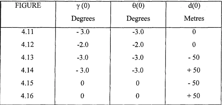
Figures 4.11, 4.16 : ILS responses in the presence of atmospheric disturbances for the
glide-path system
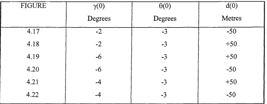
Figures 4.17, 4.22 : MLS responses for the glide-path system
Figure 4.23 ; Block diagram of a noise signal
Figure 4.24 : MLS responses in presence of sensor noise for the glide-path system
Figure 4.25 : MLS responses in presence of sensor noise with the addition of a filter
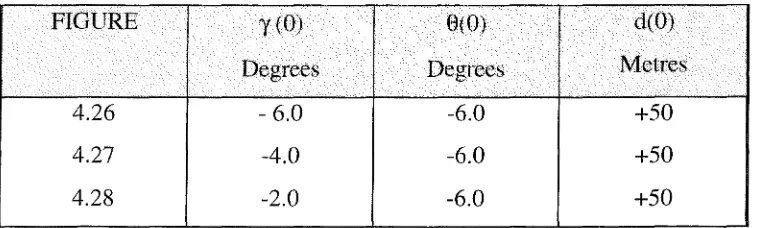
Figures 4.26, 4.28 : GPS responses with a 2 seconds loss of information for the glide-path
system
Figures 4.29, 4.31 : GPS responses with a deficiency of 3 metres in the receiver accuracy
for the glide-path system
Figure 4.32 : Localiser control system
Figure 4.33 : Block diagram of the localiser-coupled control system
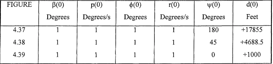
Figure 4.34 ; ILS responses for the localiser system
Figure 4.35 ; Representation of a sidegust
Figure 4.36 ; ILS responses in presence of side gusts for the localiser-coupled system
Figures 4.37,4.39 : MLS responses for the localiser system
Figures 4.41, 4.42 : MLS responses in presence of side gusts for the localiser system
Figure 4.43 : MLS responses with capture logic
Figures 4.44, 4.46 : MLS responses in presence of sensor noise for the localiser system
Figures 4.47, 4.48 : GPS responses with a 2 seconds loss of information for the localiser
system
Figures 4.50, 4.52 : GPS responses with a deficiency of 3 metres in the receiver accuracy
ACRONYMS AND ABBREVIATIONS
A / C : Aircraft
A f C S : Aircraft Flight Control System
c.g: Centre of gravity
comm : Command
DGPS : Differential Global Positioning System
DH : Decision Height
DoD : Department of Defence
FANS : Future Air Navigation Systems
( r f : Glide-Path
GPS: Global Positioning System
ICAO: International Civil Aircraft Organization
ILS: Instrument Landing System
MLS : Microwave Landing system
ph: Phugoid mode
r e f : Reference
RVR: Runway Visual Range
R X : Receiver
S A S : Stability Augmentation System
sp : Short period mode
T X : Transmitter
UHF: Ultra High Frequency
VHF: Very High Frequency
INTRODUCTION
Aircraft automatic landing systems are used when the weather conditions are so
bad that visibility for a pilot is so impaired that it would not be possible to land his aircraft
safely, even though not to do so implies, at worst, a diversion to another airport with better
visibility, and all the inconvenience such a change of landing implies for passengers and
airline alike, or, at least, another landing attempt at the same airport but in visibility which
may be worse than the first attempt, with all the implications that such a situation has for
aircraft safety.
In Europe, in particular, there is considerable economic benefit in equipping large
passenger aircraft with automatic landing systems which will ensure that landing at the
intended airport will take place no matter what is the visibility.
Aircraft instrument procedures currently use Very High Frequency Omnirange
(VOR), Instrument Landing System (ILS) and Distance Measurement Equipment (DME)
for approach and landing. The approaches are straight and the flight path angle is fixed at a
value of about 3°. But, since the first automatic landing in 1965, the growth in air traffic
has been so great that there is now being experienced at most large airports considerable
difficulty in handling the present levels of traffic. An alternative solution, which permits a
greater number of aircraft to use the existing runways, is to execute curved approaches
using either the Microwave Landing System (MLS), which is a ground based system, or
the Global Positioning System (GPS), which is a satellite navigation aid. Using GPS
would avoid the expense of having to equip every airfield and maintaining and updating
any ground equipment associated with MLS. However, since GPS is a system owned by
the US DoD and its availability cannot be guaranteed, Europe cannot depend solely on this
device for navigation information. Thus, MLS is still a viable system for widespread
implementation.
The purpose of this research was to evaluate the dynamic performances of an
automatic landing system using either ILS, MLS or GPS. This dissertation begins with a
brief description of a 3-axes aircraft flight control system (AFCS) for use with a
INTRODUCTION
ILS, MLS, and GPS follows, before the presentation of details of a simulation of the
Boeing-747 on approach and then for the automatic landing system. System design,
analysis and implementation have been carried out utilizing Matlab and the Control
System Toolbox. The control systems incorporated the ideas of feedback and linear
analysis. Since the longitudinal and lateral motions of the aircraft have been treated
separately, a glide-path control system and a localiser control system were designed. All
the tests were carried out for a number of different entry conditions and in presence of
perturbations like atmospheric turbulence or sensor noise.
A particular feature of the research reported here was the design of a single
automatic landing system, also capable of producing automatic approaches, suitable for
use with the Boeing-747 but with the option of using as the path-deviation sensor a radio
receiver operating with the ILS, or the MLS, or GPS. All the results presented here were
based upon simulations of the Boeing-747 aircraft dynamics, its corresponding
closed-loop attitude control systems, and the path-deviation-coupled automatic control system.
ILS, MLS, and GPS were selected independently with appropriate entry conditions,
IVtlFUCfLAfnTIFLICiHTrCDCMSnnRflL STfSmEAd
1 Aircraft flight control system (AFCS)
Control is necessary for any flight. Without a stabilizing control, an aircraft after a
disturbance, will not necessarily come back to its initial position ie there can exist a steady
state error; if the aircraft does turn to the initial attitudes, it may do so only after too long a
period. Conventionally, there are controls for pitch, roll and yaw, which affect motion
about the transverse, the longitudinal and the normal axes. These controls are also used to
minimise the effects of various disturbing factors. A flight control system will include
actuators, sensors and controllers as well as the aircraft dynamics. A structure of such a
system is shown in Figure 1.
Controller Actuator A/C Dynamics desired + error
output *(~) •Gc(s) "^Gservo(s) \G(s)
measured output Ksensor motion signal Sensor
Figure 1.1
The actuators operate on the aircraft control surfaces (elevator, aileron, rudder), which are
used for steering. In earlier days, only mechanical actuators were used : pitch and roll
controls were activated by means of the yoke and to deflect the rudder the pilot moved his
pedals in the cockpit. The yoke and pedals of the primary flying controls required the pilot
to maintain a counterforce for steady manoeuvres. With large transport aircraft such as
Boeing-747, it is impossible for a pilot to sustain the force required. Consequently,
electrohydraulic actuators have been introduced. The command signals to these
electrohydraulic actuators are electrical voltages supplied from the controller of an AFCS.
1 AIRCRAFT FLIGHT CONTROL SYSTEM
Therefore, the actuator dynamics have been represented by a simple transfer function :
Gservo(s) = - ^ ^ = K (1.1)
8,(3)
More specifically, Gservo(s) has been taken as 1°/V.
Sensors provide measures of any changes in motion variables such as pitch angle, roll rate
etc. Changes in motion usually occur either in response to a pilot's commands or to an
encounter with some disturbance, or in response to both. The signals from these sensors
are used as feedback signals for the AFCS. The sensors are frequently represented by their
sensitivities, viz.
— = Ksensor, (1.2)
y
which is dimensional. In this project, the sensors have been considered as ideal;
i.e. I Ksensor I =1. (1.3)^
An AFCS compares the commanded (or desired) motion with the measured motion and, if
there is any difference, generates in accordance with the required control law, the signal to
the actuator to produce the appropriate control surface deflections to bring the measured
motion into correspondence with the commanded value (Draper, 1981).
2 /uunMOAA/mcuitnoitrG sifSTinvi
2.1 Presentation
An automatic landing system is used to cause an aircraft to descend to a minimum height
without any human intervention and in low-visibility. A classification for such landings
exists and is detailed in Table 2.1 :
DH RVR
Category I 60 m > 800 m
Category II 30 m > 400 m
Category III
a < 30 m > 200 m
b < 30 m > 50 m
c < 30 m = 0 m
Table 2.1
The automatic approaches are prohibited unless horizontal visibility, called " runway
visual range " (RVR) exceeds a published threshold. The crew must execute a missed
approach if the runway lights are not visible when the descent reaches a published
" decision height " (DH). In the case of Category III aircraft, a missed-approach is not
allowed below the DH. Therefore, the automatic landing system and all the equipment on
2/ULrrCHVL4Tl(:i,A}f[H]yGSlfSTnEM
An automatic landing system comprises a number of different stages (McLean, 1990),
which are summarized in Figure 2.1 a :
P o i n t
1 O u t e r m a r k e r r a d i o b c a c o n 2 M i d d l e m a r k e r r a d i o b e a c o n 3 S t a r t of f l a r e p h a s e
4 S t a r t of K O D m a n o e u v r e 5 P o i n t o f t o u c h d o w n
2 0 0 ft
m h n r d s h i n i l d c r 7 5 ft
R u n w a y c e n t r e - l i n e
5 0 m
8 m h a r d s h o u l d e r
0 0 0 m 3 0 0 0 m r u n w a y l e n g t h F l a r e A p p r o a c h
F i n a l a p p r o a c h
Figure 2.1 a
- During the approach, the aircraft is guided along the glide path by a glide-path-coupled
controller and is steered onto the runway centre-line by means of a localizer-coupled
control system.
- The flare manoeuvre is initiated once the aircraft has descended to about 50 ft altitude.
The trajectory represents the path of the aircraft's wheels and has normally an exponential
shape (see Figure 2.1 b).
The equation which governs this trajectory is :
h == h,.e-"T CZ.l)
where is the flare entry height and T is the time constant of the exponential flare.
G l i d e p a t h c e n t r e - l i n e
P o i n t of t o u c h d o w n
R u n w a y t h r e s h o l d
G r o u n d
2 AUTOMATIC LANDING SYSTEM
- The last stage of the flight is at touchdown when a command signal is applied to the
elevator to lower the aircraft's nose to bring the nose wheel into contact with the runway.
At this point, too, if any drift has built up in the lateral path, this is removed by the pilot
executing a kick-off drift manoeuvre.
In this project, the Instrument Landing System (ILS), the Microwave Landing System
(MLS), and the Global Positioning System (GPS) are discussed. ILS equipment is
installed at every major airport and most commercial aircraft are equipped with airborne
equipment which can receive the transmitted information. MLS is more accurate than the
present ILS and has been recommended as its successor. Although there is no technical
problem in replacing ILS with MLS, setting-up is quite slow for a number of reasons
explained later in this chapter. GPS navigation has been recognised by the entire ICAO
membership as the future air navigation system. It greatly improves navigation precision
and covers the entire world. But, because it remains under US DoD control, its
development for commercial aircraft in Europe remains uncertain, although its use as a
2 AUTOMATIC LANDING SYSTEM
2.2 Instrument Landing System
The Instrument Landing System (ILS) has been the standard landing aid since 1948. It is
only used with runways of length greater than 1800 m and is categorized as Category II or
III. The approach trajectory is linear with a glide path angle about 3°. Its height above the
runway threshold will be 15 m and the touchdown point will be 300 m from the threshold.
This ideal trajectory is at the intersection of two planes (Alari, 1987) and is illustrated by
Figure 2.2 :
- the localiser (LOG) defines a vertical plane (plane V). It provides information about
whether an aircraft is to the left or to the right of the runway centre-line.
- the glide path transmitter (GLIDE) defines a slanting plane (plane G) and provides
information about whether an aircraft is flying above or below the glide path.
3nt V L O G
Figure 2.2
The system also provides distance information referenced to the runway threshold. Three
marker beacons are located at nominal locations (see Figure 2.3) :
- 7200 m (outer marker)
- 1050 m (middle marker)
2 AUTOMATIC LANDING SYSTEM
The marker beacons operate at a frequency of 75 MHz; the modulation frequencies for the
outer, middle and inner markers are 400, 1300 and 3000 Hz respectively.
By passing over the marker beacons, the marker receiver produces audio signals (MORSE)
and displays visual signals (colours) in the aircraft cockpit (Combes, 1993).
'TT^T^TTTTTT/TTTTTTTT? ioiS.
MORSE :
Colours: white amber
Figure 2.3
blue
The transmitters LOG and GLIDE operate in frequency bands of 40 channels as follows :
-LOG : 108-112MHz (VHF)
- GLIDE : 329-335 MHz (UHF)
The ground transmitter (VHF or UHF) transmits amplitude modulated signal at frequencies
of 150 and 90 Hz (see Figure 2.4). The difference between the modulated signals (DDM) is
proportional to the angular deviation ( a or 9). If the amplitude modulated signal are called
a and b, with a < b respectively, and if m (equal to 0.4 for ILS transmitters) is the depth of
modulation,
then :
ddm = m*(a - b) / (a+b) = 0.4* (a-b) / (a+b) (2.2)
2 AUTOMATIC LANDING SYSTEM
fl»n^ GU 1 JOOm
V I
\
90j SSH >C.4
SO)
Figure 2.4
ILS has a coverage illustrated in Figure 2.5 :
In the lateral plane, the following hold ;
- for the localiser, the coverage is ± 1 0 ° up to a range of 25 nm and ± 35° up to a
range of 17 nm.
- for the glide : ± 8° up to a range of 10 nm.
For the vertical plane, the parameters are :
- for the localiser, ILS covers from 0 to 7°.
2 AUTOMATIC LANDING SYSTEM
t35°
4^10°
-2-5flm J runway centre-line
- 1 0 ° 10 nm 17 nm 25
LOC antenna
-35°
runway centre-line G
\ G L I D E Diane
fl 45 Y
G is at the intersection between the ideal trajectory and the ground.
Figure 2.5
The ILS system has a number of limitations at present but it is not now possible to
improve it any further. These limitations include ;
- single aircraft approach;
- restricted coverage; beam capture problems.
- large antennas; implementation problems.
- high sensitivity to unwanted reflections and interference.
2 AUTOMATIC LANDING SYSTEM
2.3 Microwave Landing System
With this system (CAA, 1988), several simultaneous approach paths are possible.
Segmented and curved approaches with various glide path angles are available. The
aircraft's position is accurately known as a consequence of the permanent distance
information given by the DME (Distance Measurement Equipment) or DME/P system (P
stands for precision).
There are five ground stations (see Figure 2 . 6 ) :
- a front azimuth station (AZ) at the far end of the runway and located on the centre-line,
- a back azimuth station ( B K AZ) located at the runway threshold,
- an elevation station (EL) located at 300 m from the runway threshold and to the left of
the runway,
- a station for the flare manoeuvre (FL) at 1000 m from the runway threshold,
- and a DME or DME/P station.
BK A2
2 AUTOMATIC LANDING SYSTEM
The first four stations take it in turns to operate at a frequency of about 5 GHz (C-band or
SHF) on 200 channels. A whole cycle lasts 64 ms (see Figure 2.7).
0 5 10 26 31 36 54 59 64 ms
i EL 1
FL AZAV FL EL AZ ARorDATA EL FL
Figure 2.7
The MLS uses a technique called Time Reference Scanning Beam (TRSB), the principle
of which is explained in the following section (Kelly, 1976) and is illustrated in Figure 2.8
(which is the special case of the AZ station).
Each transmitter (AZ and EL) produces a narrow beam (l°-3°), which is rapidly scanned
to and fro or up and down across the coverage region. The lateral and vertical position of
the aircraft within the sector is determined by the time difference between the beams
crossing the aircraft's antennas.
On board, the signals are received on a single UHF receiver, decoded and sent either
directly to a ADI (Attitude Director Indictor) or to a navigation computer.
Front AZ station ;
2/LUT0]VUlTTK:iJ\*f[W}fG STfSTTEM
On-board:
forward beam
> t, time
ackward beam
At is the time difference between the reception of the forward and backward beams. 8 = k. (To - At)
where k is the angular velocity of the beam.
Figure 2.8
(2.3)
DME measures the slanting range R between the plane and the ground. It is used in
conjunction with VOR (Kayton and Freid, 1969), which provides bearing (9) information^.
The DME operates in the frequency band 960-1215 MHz (UHF, L-band) and the VOR
within 108-135 MHz (VHF).
The principle is the same as for a secondary radar but in the reverse direction. The ground
DME station responds upon receipt of a signal from the airborne transmitter. On detecting
this signal, the station replies using a pulsed transmission, coded in MORSE, with a delay
of 50 ps. The onboard receiver measures the time difference between the to and from
signals and computes the range R viz.
c.t T
R (2 4)
2 AUTOMATIC LANDING SYSTEM
There are 2 levels of accuracy :
- ± 0.2 nm for the DME
- ± 0.02 nm for the DME/P.
The DME is rarely affected by atmospheric perturbations. The only problem comes from
its capacity, which is limited to one hundred aircraft.
Figure 2.9 gives details of the MLS coverage :
- ± 40° for the front AZ.
- ± 20° for the back AZ.
- from 1 to 7.5° for the front EL.
- from 1 to 20° for the back EL.
At the front of the runway threshold, the length is 20 nm and the height is 20 000 ft. For
the back area, the values are divided by four.
2 0 0 0 0 '
5 0 0 0
5 NM
20 NM
+ 2 0
+ 40
2 AUTOMATIC LANDING SYSTEM
Different MLS operational procedures are used :
- The basic procedure follows the same procedure as ILS but, as soon as the aircraft is in
the coverage volume, proportional instrument guidance and continuous distance
information are used.
- In the segmented procedure, guidance is provided via predetermined points (waypoints).
Segmented approaches are quite useful in areas where terrain, environment or obstacles
reduce capacity and flexibility.
- The curved procedures are similar to the segmented ones, but they require higher
tracking accuracy during turns, to provide greater navigation accuracy.
With segmented and curved procedures, the operational utilisation of the airspace is
increased, with the approach track becoming shorter, and the pilot workload reducing.
Compared with the installation costs for ILS GLIDE and LOC transmitters, setting-up of
the MLS ground stations is cheaper. But on-board the aircraft, the situation is reversed :
because there are many ground stations, more antennas are required in the aeroplane.
Furthermore, since multiple approaches are possible, it is no longer a single approach
which has to be visualized but an air traffic lane.
Hence, the setting-up of MLS is quite slow : besides the reorganization required,
compatibility between ILS and MLS must exist for the duration of any transition period
2 AUTOMATIC LANDING SYSTEM
2.4 Global Positioning System (GPS)
This system, based upon artificial satellite positions, is able to locate a mobile or fixed
station. It has been developed by the DoD of the USA for military purposes. It comprises
three sub-systems : the space segment, the user segment and the ground control segment
(Carel, 1993).
Space segment
This segment comprises 18 satellites plus 3 spare satellites and has the following
characteristics (see Figure 2.10):
- 6 quasi-circular orbits
- period of a satellite : T = 1 l h 5 7 ' 5 8 "
- altitude : h = 20180 km
- orbits have an inclination of 55° (reference is equator)
- 1 2 0 ° longitude angle between each satellite
- anywhere in the world, 5 satellites can be used simultaneously (11 is a maximum).
- each satellite has a caesium clock synchronised to the international atomic time.
- life of each satellite is 7.5 years.
2 AUTOMATIC LANDING SYSTEM
The distribution of the satelhtes in the 6 orbital planes is shown in Table 2.2.
1 1 0 0
1 2 0 120
1 3 0 240
2 4 60 40
2 5 60 160
2 6 60 280
3 7 120 80
3 8 120 200
3 9 120 320
4 10 180 120
4 11 180 240
4 12 180 360
5 13 240 160
5 14 240 2 8 0
5 15 240 4 0
6 16 300 2 0 0
6 17 300 320
6 18 300 80
1 spare 1 0 30
5 spare 2 120 170
3 spare 3 240 3 1 0
2/iLrroM/ni(:i.AJNDr\K3 sifSTnEid
Each satellite produces its own code from the following classes :
- code C/A (Coarse Acquisition) on a frequency LI = 1575.42 MHz.
1023 bytes are generated in 1 ms. The precision is 175 m to 0.95 probability.
- code P (Precision -for military services only-) on a frequency L2 = 1227.60 MHz.
10.23 Mbytes are generated in 1 s. The precision is 37 m to 0.95 probability.
These codes allow the identification of each satellite and the measurement of the
propagation time, At, as shown in Figure 2.11.
code generated in the RX : 0 0 1 1 1 0 O i l
code received from the satellite : • 0 0 1 1 1 0 0 1 1
At,
Figure 2.11
User segment
This segment relates to the vehicle'*, the location of which is to be found in four
dimensions : latitude, longitude, altitude and universal time. On board a civil vehicle,
there are :
- a computer to process the information;
- a UHF receptor (L-band) which operates at 1575.42 MHz.
- a quartz clock, which is not synchronised to the universal time. The clock error induced
is one of the unknowns of the localisation problem.
Four satellites are required to solve the problem. Each of them gives a pseudo-range,
different from the true range, because of the RX clock bias : as it is a quartz clock, it is not
as accurate as the caesium atomic clock used in the ground segment.
The determination of the pseudo-ranges is based upon the propagation time of an
2 AUTOMATIC LANDING SYSTEM
The coordinates x,y,z (in an earth reference axis system) representing the position of the
aircraft can be computed by means of the following system :
(JT - j r , ) : 4.(jr - };): 4.(2.- 2^)= := (if, ZT,): == (/Lfi)
where
E l denotes the receiver clock bias;
Dj is the true range;
djdenotes the pseudo - range given by Atj * c or Dj + c.E^;
X ; , Y j , Z j represents the satellites'coordinates (from the ephemerides)
c is the speed of the light.
There are also secondary terms errors, including for example, the ionospheric delay^
(Kingsley and Quegan, 1992), but because such terms are very small, they are normally
ignored.
Ground control segment
This segment consists of 5 stations (see Figure 2.12):
I I
I I ! / / / / /
V,
I I M i l
W / T V V V H - W ' ' v s x m z r H
SUBZZy \ \ - ; • •7'
Figure 2.12
^ The effect of the ionosphere (from 60 km to 1000 km) on radio waves passing through it is to cause attenuation, refraction and a rotation of the plane of polarization known as Faraday roation.
2 /UUTnOO/LVT]C()0}fTTl01,SrySTnEA4
- a Master Control Station (MCS) in Colorado Springs.
- 4 others in Hawaii, Ascension, Diego Garcia and Kwajalein. These stations receive
messages from the satellites and transmit the information to the MCS, which computes the
orbit of each satellite, its position on its orbit and the corrections necessary to syncronise
their clocks. The MCS sends these results to the user segment in order to enable the
system of four equations to be solved.
Because DoD of the USA does not want civil users to have too good an accuracy, it adds
some errors. Without any Selective Availability (SA), the accuracy at the frequency
1575.42 MHz could be about 30 m. An example of SA can be the modification of the
satellites' coordinates.
Techniques have been implemented to counteract SA. Among them, there is the DGPS
(Differential Global Positioning System). The idea is to use another receiver, whose
position is known. This receiver computes the satellites'coordinates. The results from the
stations and the receiver are compared and the error is transmitted to the user segment.
One example is the DGPS developed by Honeywell and Pelorus (Canada). Three ground
receivers collect the signal from at least 4 satellites and a ground station computes the
corresponding errors, which are transmitted to the aeroplane (Daoust, 1996).
Because of its complete world coverage and its high accuracy, this system is very
attractive for use in aircraft operations. But the system is not without its disadvantages :
- during 15 min or 30 min, holes in the coverage can occur;
- a satellite may not be operational and the user may be unaware of the fact;
Z/lUTCHVUlTTKZljUfCKbJG STfSTlEM
- the operation and maintenance of the GPS is undertaken solely in the USA. Therefore,
without any notice the system could be denied at any time to all civilian users by the US
defence authorities.
To compensate for these problems, ICAO advises that GPS be coupled with another
existing area navigation system such as OMEGA or VOR/DME, although these navaids
are scheduled to be phased out in the long term.
A project to improve the space segment, is being established : a geostationnary satellite in
connection with some ground stations will check the state of the satellites. GPS will gain
3 DESIGN OF THE AUTOMATIC FLIGHT CONTROL SYSTEM
3.1 Aircraft dynamics and stability
To implement the automatic landing systems, a mathematical model has been built based
on differential equations, which describe the motion of the Boeing-747 on approach. The
equations have been linearized, which allows Laplace transforms to be used (Dorf and
Bishop, 1995). Because the topic mainly deals vwth flight control, the equations of motion
have been based on the aircraft stability axes, which are a special case of body-fixed axes
(See Figure 3.1).
U, V, W are the forward, side and vertical velocities L, M, N are roll, pitch and yaw moments
P, Q, R are the angular velocities, roll, pitch and yaw. ((), 8, y are roll, pitch and yaw angles.
£—C
.
' C ;
Figure 3.1
The aircraft dynamics are represented by a state variable model and not by a transfer
function for several reasons :
- the aircraft motion is multivariable;
DESIGN OF THE AUTOMATIC FLIGHT CONTROL SYSTEM
- a transfer function does not include any information concerning the internal structure of
the dynamic system it represents;
- state variable models lend themselves to easier computer simulation.
The system is totally defined by the knowledge of its input vector, u, its state vector, x,
and its output vector, y (see Figure 3.2).
initial conditions x(0)
input
A/C Dynamics
output ^
u(t)
f A/C Dynamics
y(t)
Figure 3.2
The rate of change of the state vector of the system relates to the state vector of the system
and the input vector, and is represented by the following equation, called a "state
equation"
x = Ax + Bu (3.1)
where
- A is a square matrix of order n*n;
- B is a matrix of order n*m;
- X is the state vector of dimension n, consisting of the state variables, which are chosen so
that they fully characterise the system.
- u is the control vector of dimension m, consisting of the control input signals.
The A matrix comprises the stability derivatives, gravity and the forward speed.
3 DiEsicHN c)F [HE ATJii:wduiTiK:];L]c;Hrr(:c)NTrR{Di,srysrrE]w
The output of the system is identified in terms of the state variables and the control input
signals. The corresponding equation is called "output equation" :
y = Cx + Du (3.2)
where
- y is the output vector of dimension p ;
- C is the output matrix of order p*n;
- D is the direct matrix of order p*m.
Disturbances like atmospheric turbulence are taken into account by adding a term to the
right hand side of the state equation thus (McLean, 1990):
x = Ax + B u + E d (3.3)
where
d represents the disturbance vector of dimension 1;
E is a matrix of order n*l.
In order to incorporate noise effects on sensors, another term can be added to the output
equation :
y = C i + Du + F.^ (3.4)
where
^ denotes the noise vector of dimension h;
F is a matrix of order p*h.
In this research, the output equation depended solely upon the state vector, viz.
D = 0. ( 1 5 )
The system relationships are represented by diagrammatic means. A software package
called Simulink has been used in conjunction with Matlab (mathematical tool box) for
control system design and analysis.
Since small perturbations were assumed, the longitudinal and lateral motions could be
3 DESIGN OF THE AUTOMATIC FLIGHT CONTROL SYSTEM
aircraft's dynamic stability are also presented. Finally, the last part of this chapter deals
with the response of the uncontrolled Boeing-747 to a step input.
Information about the dynamic stability of the aircraft can be obtained by considering the
eigenvalues of the A matrix. The ftinction, EIG, in Matlab computes these eigenvalues by
solving the equation :
|AJ.Aj = 0 (3X0
where I is a square identity matrix.
The aircraft is said to be dynamically stable if all its eigenvalues X have negative real
parts.
3.1.a Longitudinal motion
The longitudinal motion was assumed to include forward, downward and pitch motions.
Hence, the following state variables were considered :
- u, which denotes the change in forward velocity [m.s"' ];
- w, which denotes the change in vertical velocity [m.s"' ];
- q, which denotes the change in pitch rate[deg.s"'];
- 9, which denotes the change in pitch angle [deg].
The state vector x can be written as follow :
u w
q e
X = (3.7)
Since the control surfaces being considered were the elevator and the engine thrust, the
control vector u is :
' 5
u E
3 DESIGN OF THE AUTOMATIC FLIGHT CONTROL SYSTEM
The sign convention adopted for the various control deflections is illustrated in Figure
3.3.
Ru jjgr
ufCon go
00 OOCvM DO
Figure 3.3
The equations of longitudinal motion can be represented by
ii = X„u + X „ w - g 6 +Xg^8g +Xg^8TH
w = Z,u 4- w + U^q + E + Zg^8
q = M , u + M^w + M^q + ^
0 = q
where
= ( M ^ + M ^ Z J
M q = ( M q + U . M ^ )
M , , = ( M « , +
(3.9)
(3.10)
(3 11)
(3.12)
(3 J 3)
(3 J 4)
(3.15)
3 DESIGN OF THE AUTOMATIC FLIGHT CONTROL SYSTEM
The State coefficient matrix A is given by^:
0 - g "-.0209 j 2 2 0 - 4 2 2
A; = Zu Zw Uo 0 - 2 0 2 - j l 2 221 0
A; =
0 0
Mu Mq 0 401 -4018 -.357 0
0 0 1 0 0 0 1 0
and the driving matrix B is given by :
B, =
^5™
Za.
0 0
459 -6.42 - 3 7 8 0
.000057
-40000249
.00000031
0
(3.18)
(3.19)
Table 3.1 summarizes some of the results related to the longitudinal dynamic stability :
Mode Eigenvalue Natural Damping Period Settling
Frequency ratio Time
rad/s s s
Short period -j439±^6286 ^69 .577 1.3
-Phugoid -40111^1507 ^51 .0073 41.610 4536
Table 3.1
Figure 3.4 shows the pitch attitude and pitch rate responses to an unit step elevator input
with two time scales (60 and 6000 s). The corresponding open-loop block diagram is also
given.
Note that the settling time for both 9 and q corresponds to too long a period and that after
the transient response has decayed, a steady-state error exists.
3 DESIGN OF THE AUTOMATIC FLIGHT CONTROL SYSTEM
StepE
Thrust Mux
Mux B1
1/s
Sum Integral
•4
K A1
1
or
Demux -r-HI Demux -H_ theta
theta
D1 <D
X3 c
0 . 4
0.2
0
-0.2
- 0 . 4
-0.6
0 2 0 4 0
time in s
60 2 0 4 0
time in s
0 . 4
0 - 2
n) 0 0) "D C O" - 0 . 2
- 0 , 4
-0.6
0 2 0 0 0 4 0 0 0 6 0 0 0
time in s
2 0 0 0 4 0 0 0 6 0 0 0
time in s
3 DESIGN OF THE AUTOMATIC FLIGHT CONTROL SYSTEM
3.1.b Lateral motion
Lateral motion involves sideslip, roll and yaw motions, which correspond to the following
state variables :
- P, the change in sideslip [deg];
- p, the change in roll rate [ft.s"'];
- r, the change in yaw rate [ ft. s"' ];
- (p, the change in bank angle [deg].
Hence, the state vector x representing lateral motion can be expressed as :
"P"
P
(120)
r (p
The ailerons and the rudders are the control surfaces involved in lateral motion, hence the
control vector u may be written as ;
u = (3.21)
The equations of motion are :
P ~ Lpp + LpP + L^r + Lg 6 ^ + Lg^8 ^ r = N ; p + N ; p + N ; r + N ; ^ 6 , + N ; ^ 8
^ = p
8 \|) = r
(3.22)
( 1 2 3 )
(3.24)
(3.25) (3.26)
3 DESIGN OF THE AUTOMATIC FLIGHT CONTROL SYSTEM
The State coefficient matrix A can be expressed as :
A =
Y,. 0 —1 "-.089 0 - 1 j457"
Lp K l ; 0 - 1 3 9 -.975 3 2 7 0
(3.27) 0
=
j 8 6
-.975 3 2 7
(3.27)
Np N ; N : 0 j 8 6 —.166 —3 0 (3.27)
0 1 0 0 0 1 0 0
and the driving matrix B as :
B
0 Y'd. "0 .0148"
Ls, L' 2 2 7 .0636
=
4264 -.151 (3.28)
N L N L 4264 -.151
(3.28)
0 0 0 0
Table 3.2 summarizes some of the results related to lateral dynamic stability :
Mode Eigenvalue Natural Damping Period Settling
Frequency Ratio Time
rad/s s s
Spiral convergence -.0848 - - -
-Rolling subsidence -L227 - - -
-Dutch roll -.0261±j.6877 .6884 .0379 &127 192
Table 3.2
Figure 3.5 shows the roll rate and yaw rate responses to an unit step aileron command with
3 DESIGN OF THE AUTOMATIC FLIGHT CONTROL SYSTEM
m
StepE
Thaist Mux
Mux 82
1/s Sum Integra
K A23
1
or K t i a f
Demux U-H.
Demux
D) 0.05
D)
•o 0.01
- 0 . 0 5 -0.01
20 40
time in s
20 40
time in s
0.15
0.1
D) 0.05
0) "D
~ 0
-0.05
- 0 . 1
j llln' '"
200 400 time in s
600
0.04
0.03
0.02
• S 0 . 0 1 ! _ c
" 0
- 0 . 0 1
- 0 . 0 2 0 200 400
time in s
600
Figure 3.5
3 DESIGN OP THE AUTOMATIC FLIGHT CONTROL SYSTEM
The responses for p and r are dominated by the rolUng subsidence and the dutch roll
modes and converge to zero after a settling-time about 200s. Here the usual UK definition
of settling time has been used viz the time taken to settle within 1% of the final steady
value. The usual approximation of 5 X the principal time constant applies.
Without any feedback control, the Boeing-747 is seen to be underdamped, particularly for
the longitudinal motion. Therefore, the use of a Stability Augmentation System (SAS) is
3 DESIGN OF THE AUTOMATIC FLIGHT CONTROL SYSTEM
3.2 SAS and attitude control
A Stability Augmentation System (SAS) should increase the dynamic stability of an
aircraft (McRuer and Graham, 1981). Since the design of such a stabilizing control
involves full state variable feedback, attitude control system is treated at the same time.
This attitude control allows an aircraft to be placed and maintained in any required
specified orientation in space.
3 . 2 . a Longitudinal control
The method of eigenvalues assignment was chosen for the SAS design since it gives the
designer an opportunity of precisely locating the eigenvalues of the closed-loop system in
such a way that the dynamic response of the system is acceptable. The problem consists of
finding a feedback matrix, , to be used in the control law :
u = Kg .X, (3.29)
such that the eigenvalues, k y , o f the closed-loop system are placed at specified locations.
Note that the closed-loop system is defined by :
X == CA. H BiKLc):: (3.3())
Therefore the eigenvalues, X,, are determined from the characteristic polynomial, f ( l ) :
ffA.) = 1II -jAi- ISlKLc I (3 31)
To determine the feedback matrix a method involving " equating coefficients" was used :
Kg was determined by equating the coefficients of the polynomial equation (3.31) with
those of the desired polynomial, which was formed fi-om the specified eigenvalues.
In the particular case of this research, the following situation obtained :
- open-loop eigenvalues :
^ 4 4 3 9 ± i . 6 2 8 6
3 DESIGN OF THE AUTOMATIC FLIGHT CONTROL SYSTEM
desired closed-loop eigenvalues :
-.5 + j . 4
- 1 0 ± j l \ 0 7 1
which yielded to the feedback matrix, BQ,:
Kc - j 9 8 3 2 7 9 16497.426
-1.144660 -30.86533 -114.8368
-235.6975 1108199.4 12809960.3 (3.32)
The high values of feedback gains reflect the fact that one of the inputs to the aircraft
dynamics is engine thrust. These "gains" are much smaller when engine gain is factored
out.
The feedback matrix Kc was found by using the Matlab function PLACE
Kc = PLACE(A,B,P)
where
P = [-5+J*.4; -5-J*.4; -10+J*7.071; -10-J*7.071]
a n d J = SQRT(-l).
(3.33)
(3.34)
Table 3.3 presents the resulting longitudinal dynamic stability information
Mode Eigenvalue Natural Damping Period Settling
Frequency ratio Time
lad/s s
s
Phugoid -.5±j.4 .64 .78 9.817
-Short period -10±j7.071 12.22 .818 .514 .50
Table 3.3
3 DESIGN OF THE AUTOMATIC FLIGHT CONTROL SYSTEM
0 . 0 6
0.04
§
•o 0.02c
- 0 . 0 2
0 0.2 0.4 0.6 0.8 1 1.2 1.4 1.6 1.
time in s
E a04
x: 0 . 0 2
time in s
0)0.03
CD
TD
time in s
re 0 . 0 2 E E re
™0.01
3 DESIGN OF THE AUTOMATIC FLIGHT CONTROL SYSTEM
Notice that the flight path angle, y, of the aircraft is obtained from the kinematic
relationship :
= — ! — (3.35)
8(s) l + sTa
where
y = B - a ; (3.36)
a = w/Uo; (3.37)
is the aircraft time constant and equals to -0.512. (3.38)
The corresponding block diagram is given in Figure 3.7 ;
Step
n B
e
K c
c
1
1-ksT^ Y '
Figure 3.7
The results correspond now to acceptable flying qualities; ie well-damped pitch attitude 9
3 DESIGN OF THE AUTOMATIC FLIGHT CONTROL SYSTEM
3.2.b Lateral control
The lateral SAS was designed using the modem theory of optimal control, because the
design is unique and meets exactly a specified performance criterion. Eigenvalue
assignment could also have been used, but there is less assurance in assigned eigenvalues
providing required dynamic response with lateral motion, in which the modes of motion
are coupled. An optimal control system is a system whose parameters are adjusted so that
a performance index, J, has a minimum value. The performance index is of the form :
1 "
0
This problem is referred to in the literature as the "linear quadratic problem" which
requires for its solution the determination of an optimal control, u, which will minimize
the index , J, and which will control the aircraft whose dynamics are described by the state
equation (3.1), ie.
X = Ax + Bu
Q and G are weighting matrices of order n*n and m*m, respectively, which have to be
chosen by the designer.
The theory of the LQP shows that minimizing the index J with respect to the control
function u, is equivalent to solving an algebraic Riccati equation (ARE) viz.
0 = P.A + A ^ . P - P . B . G - ' . B \ P + Q (3.40)
Solving equation (3.40) provides the linear optimal control law :
u = - G - ' . B ^ . P . x = K c . x (3.41)
3 DESIGN OF THE AUTOMATIC FLIGHT CONTROL SYSTEM
where
K c is the feedback gain matrix.
The feedback matrix, K ^, used in the lateral control law was computed using the Matlab
function, LQR ie.
K c = L Q R ( A , B, Q , G )
where
Q = cUzig {.1 1().0 5.0 :u)} (3.4:!)
G = d i a g { . 1 5 . 0 } (3.43)
It was determined that:
Kc -4.182
.094
8303
4 7 6
l j 9 1 ~.485
4366
4 3 7 (3.44)
The resulting closed-loop system is characterised by the parameters quoted in Table 3.4
Mode Eigenvalue Natural Damping Period Settling
Frequency Ratio Time
rad/s s s
Spiral convergence - 4 8 4 8 - - -
-Rolling subsidence -1.227 - - -
3 CWESIGHN OFTHHEvlUTCMVLATIC FLKIHrTtZCHSnnROL STfSTlEM
Figure 3.8 gives the corresponding block diagram :
Step Xcomm
Kc
->P
-^4)
Figure 3.8
Figure 3.9 shows the closed-loop responses for roll rate, yaw rate and bank angle, which
were obtained for an unit step command input.
3 DESIGN OF THE AUTOMATIC FLIGHT CONTROL SYSTEM
1 . 5
1
o
•g
.5 0 . 5 "5.
0
- 0 . 5
0 10 20 30
time in s
40 50 60
0.1
O j #
0.06 o
r 0.04 a. OjW
0
- 0 . 0 2
# 1 1 1
_1 L J I J L
10 15 20 25 30 35 40 45 50
time in s
0.1
0.05
CTi o
-0.05
1 r
- J I I L .
10 15 20 25 30 35 40 45
time in s
50
3 DESIGN OF THE AUTOMATIC FLIGHT CONTROL SYSTEM
But, the yaw damper, just described, tends to oppose any change in yaw rate even when it
has been commanded. Therefore, to avoid such opposition, another feedback signal only
acting on the rudder has been added. This feedback signal consists of two elements ;
- a proportional controller, with a gain of value 2.0.
- a wash-out filter, whose transfer function is given by :
- (3.45)
where
T _ = 0 J 5 .
This value of wash out time constant was chosen as a compromise between good d.c.
rejection and minimal impairment of system transient response.
Figure 3.10 shows the block diagram, which incorporates the wash-out filter :
Xcomm
9;'
2 JI5s
2 JI5s
2
.15s-1-1
Wash-out Filter
Figure 3.10
Figure 3.11 shows the responses for the sideslip, the roll and yaw rates and the bank angle.
3 DESIGN OF THE AUTOMATIC FLIGHT CONTROL SYSTEM
0.5 O) o TD
re "5 X I
-&5
20 40
time in s
1.5
1
o O "D
c &5
CL
60 -0.5 20 40
time in s
6C
w 0.5
o o "D
c C L
-0.5
20 40
time in s
60 20 4^
time in s
60
4 DESIGN OF THE FLIGHT PATH CONTROL SYSTEM
The flight path control system permits the control of translation in either the normal or
lateral direction. Because there are no special control surfaces to control the translational
motion, the production of a lateral or normal displacement requires the indirect use of
attitude control systems. Consequently, flight path control systems form outer loops
around the attitude control systems.
Results for flight path control systems using ILS, MLS and DGPS to serve such
translational displacements are given in this chapter for several different entry conditions
and a number of atmospheric conditions.
4.1 Glide-Path-Coupled control system
Such a system is designed to closely control an aircraft's deviation above or below some
desired glide path.
4.1.a Generalities
The output signal from a glide path receiver in the aircraft is used as a guidance command
to the attitude control system. The aircraft's flight path angle, y, translates into a linear
displacement, d, from the desired glide path, viz.
+ T „ / ) d t (4.1)'°
where
y is the reference flight path angle which, if flown by the aircraft, would result in the
aircraft descending along the glide path.
4 DIESICHNF CNF FHE FLKSTRRIPA/THCZCMNTLROL STTSTNEAD
The signal measured by the glide path receiver is the angular deviation, F, or glide path
error.
F is expressed in radians and is defined as :
r ( . ) = ^ - d ( t )
where
- R(t) is the slant range in metres given by :
R(t) = Ro - Uo*t
- Uo - 67 m/s;
- Ro = 9000 m;
- 1 is the time expressed in seconds.
( 4 2 ) 11
(4j)
( 4 4 )
(4.5)
5 7 3
For small values of R the closed-loop system becomes unstable ( > oo). Hence, the
range must always exceed a critical minimum value, which was chosen in this work to be
200 m.
Notice that if y = yref then F = 0.
The situation is represented in Figure 4.1 :
Glide Path
@AircraA c.g
Ground
4 DESIGN OF THE FLIGHT PATH CONTROL SYSTEM
The transfer function, Gc(s), of the glide-path-coupled controller has two terms :
- a proportional plus integral term equal to :
- a phase advance term, which is introduced to provide additional stabilization. This term
was designed to be ;
z' ^ s + 1 ^
V IWs + 1 y
The controller transfer function, Gc(s), used therefore was given by :
. i ^ r . 4 s + i ^
Gc(s): 6 +
-s ; IW-s + l V (4.6)
The design of this conventional controller was based on complex frequency domain
techniques and was arranged to provide good transient response with zero steady-state
error.
Figure 4.2 shows the corresponding block diagram of the glide-path coupled system.
-ykf
8(s) rref=0
y G-P Controller
Attitude Controller
' + KA
+
+ DYNAMICS
1
l + sTa 7(8)
Kop
G-P Receiver
5 7 . 3 R
s.d(s)
Uo 5 7 3
Figure 4.2
So far, the speed of the aircraft had been assumed to be constant and equal to 67 m/s. In
practice, however, the aircraft speed will change with time, f r o m the value, Uo, at the start
4 DESIGN OF THE FLIGHT PATH CONTROL SYSTEM
In this research work :
- U o = 6 7 n i / s (4.7'
- U i = 5 2 m / s (4.8;
The time of the interval between the beginning and the end of the approach was taken as
100 s, which represents a practical value.
Hence, the change in reference speed ,uref, was defined as :
u«((t) = -.33t + 67.0 (4.9)
In order that the change in aircraft speed would correspond with the appropriate speed
schedule, uref(t), an aircraft speed control system was added to the glide-path coupled
control system.
The speed of the aircraft was controlled by changing the thrust, 5 , of the engines. The
transfer function representing the engine dynamics, GE(S), w a s assumed to be linear and was approximated as follows :
(}E(S) = (4.1())
l + sTc
where
- T E = 1 S (4.11)
- K E = 3 5 0 0 0 N/rad (4.12)
KE was determinated in the following way :
The excess thrust of an aircraft is given by :
W
TEXCESS = T M A X (4.13)
L / D
where
- T M A X denotes the maximum thrust fi'om the engines. F o r the Boeing-747, T M A X
approximately equals 800 000 N;
4 DESIGN OF THE FLIGHT PATH CONTROL SYSTEM
Hence :
TEXCESS = 525 000 N. (4.14)
The maximum throttle deflection, Omax, was assumed to be 1.5 rad and the control
authority, r|, was restricted to 10 %., For this authority figure, the engine gain was given
by ;
K E = 7 7 * TEXCESS . 9 , , le.
KE=35000N.rad
(4J5)
(4.16)
The transfer function, G'^ , of the speed controller was defined as ;
G'c(s) = K c / ( l + ^ )
Kc, = 25
and Kg = 0.1
OLI?)
where the controller gains were designed to be :
BL18)
(4.19)
The design was based on complex frequency methods and was arranged to provide
acceptable transient response - minimal overshoot, no oscillation, rapid rise time and short
settling time.
Notice that the speed control law involved an integral term thereby which eliminated any
steady-state error.
The feedback was based upon sensed airspeed and sensed acceleration. A block diagram of
the speed control system is shown in Figure 4.3.
Speed Controller
Engine Dynamics
(7c
'THROTTLE (S) GE(s) f XH
Accelerometer
K . . . S
1.0
AJC Dynamics
Speed sensor
4 DESIGN OF THE FLIGHT PATH CONTROL SYSTEM
4.1.b Use of the ILS
The dynamics of the ILS ghde-path receiver were considered to be instantaneous even
though it contains filters for the 90 Hz and 150 Hz modulation components of the glide
path signal. The receiver transfer function was represented by its sensitivity, KGP, viz :
0L2O)
The reference flight path angle was 3°.
4.1,b.(i) Responses for different entry conditions
The system responses for the initial values of pitch attitude, 0, flight path angle, y,
displacement, d, are shown in Figures 4.4 to 4.9 for the approach entry conditions given in
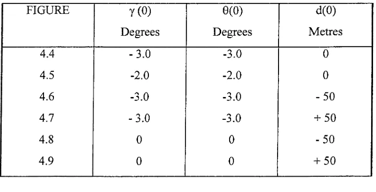
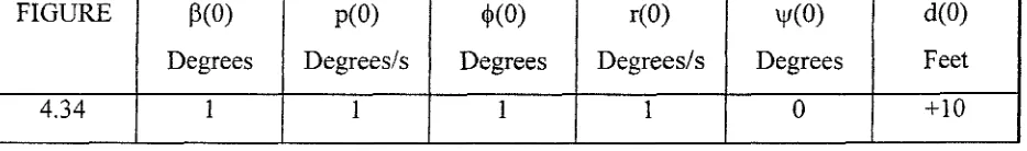
[image:57.596.53.433.417.611.2]table 4.1.
FIGURE Y(0) 8(0) d(0)
Degrees Degrees Metres
4.4 - 3 4 -3.0 0
4.5 -2.0 -2.0 0
4.6 -3.0 -3.0 - 5 0
4.7 - 1 0 -3.0 + 50
4.8 0 0 - 5 0
4.9 0 0 + 50
Table 4.1
In every case, the glide path angle, y, converged to a value equal to or very close to the
desired value, -3°. It can be seen from the figures that the responses for 6, d and F often
4 DESIGN OF THE FLIGHT PATH CONTROL SYSTEM
Steady-State errors, the dynamic responses with the glide-path coupled control system were
all satisfactory, and corresponded to acceptable performance for the closed-loop system. It
should be noted, that the aircraft had to produce very large changes in flight path angle for
the extreme "incorrect" entry conditions being applied ( See Figures 4.8 and 4.9).
In the following figures Lambda denotes the beam error, F
Figures 4.5 - 4.9
/ k l l - ' L 2 2
4^24-'LSI
4 J 4
4k36-'L42
4 DESIGN OF THE FLIGHT PATH CONTROL SYSTEM
0
- 5
CO
2
1 - 1 0
E •o
- 1 5
- 2 0
20 40 time in s
: : / l = ^
•' /
1000 2000 3000 4000 R in metres
o ) - 0 . 1
Q
(8 —0.2
I
- - 0 . 3-0.4
20 40 time in s
t %
is U
1000 2000 3000 R in metres
4000
Y(Uj = -3.U"
6(0) = -3.0"
d(0) = 0.0 m
4 DESIGN OF THE FLIGHT PATH CONTROL SYSTEM
CD-2.5
="-3.5
2
0
10
1-2
.5 •D
- 4
- 6
20 40 time in s
^ 5
^ 5 A
/
||4
1000 2000 3000
R in metres
4000
0.05
D) 0
m 0
c
ro -0.05
1
- - 0 . 1
-0.15
20 40
time in s
] kril'
1000 2000 3000
R in metres
4000
7(0) = -2.0°
6(0) = -2.0°
d(0) = 0.0 m
Figure 4.5
4 DESIGN OF THE FLIGHT PATH CONTROL SYSTEM
0
-10 g-O)
i - 3 0
.5
T3 -40 -50
- 6 0
20 40 time in s
,
0
£ „
CO 0 1
CO
o)_2
0
1000 2000 3000 4000 R in metres
0
- 0 . 2
e
c - 0 . 4 ro
S - 0 . 6
- 0 . 8
- 1
20 40 time in s
60
A
\ Uo*
1000 2000 3000 4000 R in metres
y(0) = -3.0°
8(0) = -3.0°
d(0) = -50.0 m
4 DESIGN OF THE FLIGHT PATH CONTROL SYSTEM
5
2" °
D
-5 - 5
I
JZ
" - 1 0
-15
60 40
in
2 20 a> fc .5 0
T)
-20 -40
20 40