University of Warwick institutional repository: http://go.warwick.ac.uk/wrap
A Thesis Submitted for the Degree of PhD at the University of Warwick
http://go.warwick.ac.uk/wrap/57737
This thesis is made available online and is protected by original copyright.
Please scroll down to view the document itself.
Library Declaration and Deposit Agreement
1. STUDENT DETAILS
Please complete the following:
Full name: ………. University ID number: ………
2. THESIS DEPOSIT
2.1 I understand that under my registration at the University, I am required to deposit my thesis with the University in BOTH hard copy and in digital format. The digital version should normally be saved as a single pdf file.
2.2 The hard copy will be housed in the University Library. The digital version will be deposited in the University’s Institutional Repository (WRAP). Unless otherwise indicated (see 2.3 below) this will be made openly accessible on the Internet and will be supplied to the British Library to be made available online via its Electronic Theses Online Service (EThOS) service.
[At present, theses submitted for a Master’s degree by Research (MA, MSc, LLM, MS or MMedSci) are not being deposited in WRAP and not being made available via EthOS. This may change in future.] 2.3 In exceptional circumstances, the Chair of the Board of Graduate Studies may grant permission for an embargo to be placed on public access to the hard copy thesis for a limited period. It is also possible to apply separately for an embargo on the digital version. (Further information is available in the Guide to Examinations for Higher Degrees by Research.)
2.4 If you are depositing a thesis for a Master’s degree by Research, please complete section (a) below. For all other research degrees, please complete both sections (a) and (b) below:
(a) Hard Copy
I hereby deposit a hard copy of my thesis in the University Library to be made publicly available to readers (please delete as appropriate) EITHER immediately OR after an embargo period of ………... months/years as agreed by the Chair of the Board of Graduate Studies. I agree that my thesis may be photocopied. YES / NO (Please delete as appropriate)
(b) Digital Copy
I hereby deposit a digital copy of my thesis to be held in WRAP and made available via EThOS. Please choose one of the following options:
EITHER My thesis can be made publicly available online. YES / NO(Please delete as appropriate)
OR My thesis can be made publicly available only after…..[date] (Please give date)
YES / NO(Please delete as appropriate)
OR My full thesis cannot be made publicly available online but I am submitting a separately identified additional, abridged version that can be made available online.
JHG 05/2011
3. GRANTING OF NON-EXCLUSIVE RIGHTS
Whether I deposit my Work personally or through an assistant or other agent, I agree to the following: Rights granted to the University of Warwick and the British Library and the user of the thesis through this agreement are non-exclusive. I retain all rights in the thesis in its present version or future versions. I agree that the institutional repository administrators and the British Library or their agents may, without changing content, digitise and migrate the thesis to any medium or format for the purpose of future preservation and accessibility.
4. DECLARATIONS
(a) I DECLARE THAT:
I am the author and owner of the copyright in the thesis and/or I have the authority of the authors and owners of the copyright in the thesis to make this agreement. Reproduction of any part of this thesis for teaching or in academic or other forms of publication is subject to the normal limitations on the use of copyrighted materials and to the proper and full acknowledgement of its source.
The digital version of the thesis I am supplying is the same version as the final, hard-bound copy submitted in completion of my degree, once any minor corrections have been completed.
I have exercised reasonable care to ensure that the thesis is original, and does not to the best of my knowledge break any UK law or other Intellectual Property Right, or contain any confidential material.
I understand that, through the medium of the Internet, files will be available to automated agents, and may be searched and copied by, for example, text mining and plagiarism detection software.
(b) IF I HAVE AGREED (in Section 2 above) TO MAKE MY THESIS PUBLICLY AVAILABLE DIGITALLY, I ALSO DECLARE THAT:
I grant the University of Warwick and the British Library a licence to make available on the Internet the thesis in digitised format through the Institutional Repository and through the British Library via the EThOS service.
If my thesis does include any substantial subsidiary material owned by third-party copyright holders, I have sought and obtained permission to include it in any version of my thesis available in digital format and that this permission encompasses the rights that I have granted to the University of Warwick and to the British Library.
5. LEGAL INFRINGEMENTS
I understand that neither the University of Warwick nor the British Library have any obligation to take legal action on behalf of myself, or other rights holders, in the event of infringement of intellectual property rights, breach of contract or of any other right, in the thesis.
Please sign this agreement and return it to the Graduate School Office when you submit your thesis.
Aperiodically forced oscillators
A Hau Gin
A thesis submitted in fulfilment of the requirements for the degree of Doctor of Philosophy
Mathematics Department, University of Warwick
Contents
Dedication . . . 6
Acknowledgements . . . 6
Declaration . . . 6
1 Motivation and Introduction 7 1.1 Motivation . . . 7
1.2 Introduction . . . 8
2 Uniform Hyperbolicity 11 2.1 Preliminaries . . . 12
2.2 Linear non–autonomous systems . . . 12
2.3 Functional analysis and exponential dichotomy . . . 14
2.3.1 Exponential dichotomy . . . 14
2.3.2 Green functions and bounds on response for certain types of forcing . . . 19
2.3.3 Continuity of the splitting . . . 22
2.3.4 Set of uniformly hyperbolic systems and pseudo–orbits . . 30
3 Normal Hyperbolicity 36 3.1 Normal hyperbolicity and invariant manifolds . . . 36
3.2 Computing the invariant manifold . . . 38
3.2.1 Two operators . . . 38
3.2.2 Definition of Normal Hyperbolicity . . . 40
3.2.3 Assumptions and Conditions . . . 42
3.2.4 Continuation . . . 44
3.2.5 Path–wise approach to computing invariant manifold . . . 47
3.2.6 Hybrid approach to computing invariant manifold . . . . 51
3.2.7 Graph transform approach to computing invariant manifold 55 3.2.8 Comparisons of methods that compute invariant manifolds 57 4 Synchronisation of non–autonomous oscillators 59 4.1 One oscillator . . . 61
4.1.1 Synchronisation of a forced oscillator . . . 61
4.1.2 Reliability of one oscillator systems . . . 63
4.2.1 Synchronisation of many oscillators . . . 64
4.2.2 Reliability ofmoscillator systems . . . 65
5 Application 67 5.1 Aperiodic oscillators . . . 67
5.1.1 Perturbed system . . . 69
5.1.2 Pseudo–codes for physical systems . . . 69
5.1.3 Discretisation details . . . 73
5.2 A simple 2–D oscillator . . . 86
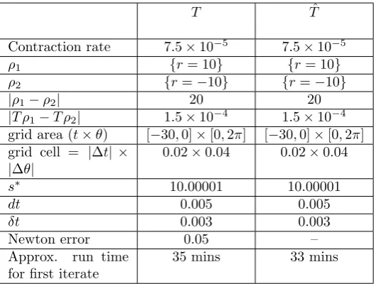
5.2.1 Contraction rate ofT and ˆT . . . 87
5.2.2 Iterates ofT and ˆT . . . 88
5.2.3 Dynamics on the invariant manifold . . . 90
5.2.4 Numerical results . . . 90
6 The Morris–Lecar model 95 6.1 Equations and parameters . . . 95
6.2 New coordinate system . . . 98
6.2.1 Adjoint method . . . 98
6.2.2 Coordinate change . . . 99
6.2.3 Perturbed Morris–Lecar system in the new coordinate sys-tem . . . 100
6.3 Algorithms adapted to the new coordinate system . . . 101
6.3.1 Rescalingw . . . 102
6.4 Periodic, two–frequency–periodic and modified Poisson spike train inputs . . . 102
6.4.1 Periodic forcing . . . 102
6.4.2 Two–frequency–periodic forcing . . . 105
6.4.3 Numerical results for periodic forcing . . . 106
6.4.4 Modified Poisson spike train . . . 113
6.4.5 Numerical results for spike train input . . . 117
7 Conclusions and discussions 124 7.1 Uniform hyperbolicity . . . 124
7.2 Normal hyperbolicity . . . 125
7.3 Synchronisations . . . 125
7.4 Applications . . . 126
Dedication
I dedicate this thesis to You God. Thank You for your faithfulness and
provi-dence. You gave me the strength and the will to keep going and stay focussed on the goal. You blessed me with incredibly kind people at every step! Thank
You for forgiving me for thinking that I can make it without You and teaching me the valuable lesson that pride comes before a fall. Thank You God that in
your Fatherly love You still receive this far from perfect thesis as an offering! I say this in Jesus’ name, the name above all names, Amen!
Acknowledgements
I thank my thesis supervisors for their help and support throughout the course
of my doctoral study. In particular, it has been an inspiration to work with Robert MacKay and I am very grateful for his direction. I am indebted to him
for his time, care and interest in my research. I am also thankful for Magnus
Richardson for his supervision and especially his encouragement when I needed it most. I would like to express my gratitude to him for setting up the
Theoret-ical Neuroscience Group which has been stimulating and motivating for us all. I would like to thank those in TNG who have contributed to my research
ex-perience, especially Azadeh Khajeh-Alijani, Naveed Malik and Robert Gardner who gave me much enjoyment and interesting conversation in the field. Special
thanks to Rupert Swarbrick and Michael Korotyaev for their valuable support in computer programming and Yi Chan for general proof–reading of this thesis.
Many thanks to those family members and friends who have given me moral
support and spurred me on to the completion of this thesis. I would also like to thank Jianwen Zhang for her support in many ways.
I would also like to mention those Ph.D friends such as Yuxin Yang, Wu Bo, Patrick O’Callaghan and Umar Hayat who have made my study an enjoyable
experience. Thanks to the Warwick University Badminton team, in particular team mates such as Andy Hotchen, Nikko Cheung and Matthew Seeley, for
providing me much enjoyment in training and games. Special thanks to the Coventry Chinese Christian Church and the youth group for giving me
memo-rable times during my study.
Declaration
I declare that, to the best of my knowledge, the material contained in this thesis is original and my own work except where otherwise indicated, cited, or
Chapter 1
Motivation and
introduction
1.1
Motivation
The motivation of this project is synchronisation at the network level. The
emerging behaviour of synchronisation is ubiquitous in science, nature and en-gineering. It is found in systems as diverse as clocks, flashing fireflies, cardiac
pacemakers, bursting neurons and applauding audiences (PRK01).
This phenomenon has received much attention from many generations of re-searchers dating as far back as 1665 when Christiaan Huygens recognised it in
his clocks. However, possibly the earliest record of synchronisation may be found in the book of Joshua in the Bible when the Israelites besieged the ancient city
of Jericho around 1200 B.C. In brief, the Israelite army was ordered to surround the city wall and at a trumpet signal, shouted out in unison. It is possible that
the soldiers synchronised with their nearest neighbours to produce a powerful output of synchronised sound, which forced the wall to crumble down and the
city was subsequently captured. It is unlikely that the ancient generation knew or understood synchronisation to the extent that they would have been able to
exploit it.
The beauty of this phenomenon is that it is very easily recognised by the
300 neurons, works rhythmically helping us to breathe subconsciously in a ro-bust and controllable way. However, there can be neuronal dysfunctions such
as in sleep apnoea and possibly sudden infant death syndrome (FN06). Thus to be able to understand and control this dysfunction would be highly beneficial
to humanity.
The Millennium Bridge in London has shown an undesirable effect termed
Syn-chronous Lateral Excitation where, as the number of walkers on the bridge increases, the bridge reaches a critical mass and starts to sway causing danger
to the walkers (Mil). It was due to subsequent research taken that a sensible solution was found and modification of the bridge was made by placing lateral
dampers under the bridge deck.
The advancement of computer technology has provided us valuable tools to observe what happens at the network level. For example, we can take a very
complicated neuron model and wire many of them together using a computer program to see what properties can arise (BRS99). However, to gain real
un-derstanding we need to tackle the problem using analytical tools (Str01). This is a highly difficult task and simplification is inevitable. Reducing the network
to just two oscillators is a natural first step. However, for the case of many oscillators, major advancement was made by Kuramoto when he considered a
simplified phase model with all-to-all autonomous coupling (Kur84). The sys-tem was shown to synchronise as it passes a critical mass which provides greater
understanding for the Millennium bridge problem.
However, the Kuramoto phase model is too simplistic and a more realistic ap-proach can be taken which includes the change in amplitude. This motivated
my thesis project and led me to consider aperiodically forced oscillators. This is of great interest because the oscillator can receive inputs from other oscillators
in the network with unknown architecture and these inputs are unlikely to be periodic and can be treated as time–dependent. This will be very useful for the
study of synchronisation of non–autonomous oscillators at the network level.
1.2
Introduction
Oscillations are ubiquitous in nature (Str04, Win80) and the theory of nonlinear
oscillators is very useful in the study of these phenomena (GH83, HS74). Au-tonomous systems of ordinary differential equations that possess a limit cycle are
commonly employed to model the individual oscillator. In reality, these systems are invariably subjected to time-dependent influences. The case of time-periodic
tongues (PRK01). However, periodic forcing is a poor representation of many real situations and relatively little attention has been paid to the case of general
bounded time-dependent forcing.
For weak time-dependent forcing, not necessarily periodic, the response of a hyperbolic limit cycle oscillator is clear from the theory of normal hyperbolicity
(HPS77, Fen71). In the time–extended space, the limit cycle becomes a
nor-mally hyperbolic cylinder which persists when weakly forced.
To be more specific let us first take the following phase coordinate system based at the unperturbed limit cycle of period, T, say. For every pointγ on the cy-cle we give it an angle θ∈ R/TZwhich is the time it takes for the trajectory
to reach γ from a reference point on the cycle. To extend this away from the cycle we can take a tubular neighbourhood of any transverse bundle (a possible choice is the vector bundle defined by taking the tangent space to the invariant
foliation, a.k.a “isochron”, at the base point on the cycle). Then any point that lies on the transverse fibre based atγcan be assigned the same angle as that of
γand we can take its relative positionr∈Rnfromγto complete the coordinate
system, where the dimension of the system isn+1. The unperturbed limit cycle is given byr= 0 and we can write the perturbed system in the neighbourhood of the unperturbed limit cycle as
˙
θ= Θ(θ, r, t) ˙
r=R(θ, r, t). (1.1)
In the unperturbed case, Θ and R are independent of t, Θ(θ,0, t) = ω = 1/T
and R(θ,0, t) = 0. We assume that Θ and R are C1. The unperturbed limit cycle ishyperbolic if the time-T map of the linearised unperturbed dynamics
˙
ξ=Rr(ωt,0, t)ξ, ξ∈Rn (1.2)
has no eigenvalue on the unit circle. The application here will be to stable
oscil-lators, thus the case of interest is when the spectrum is inside the unit circle but the theory applies equally well even if there is some spectrum outside too. Since
non–compact version of (HPS77, Fen71) is required.
This is fine as theory, but in practice one would like to know how close the cylinder is to the unperturbed one and to what extent the dynamics on the
cylinder change. To achieve realistic estimates, I shall present an path–wise approach to computing the perturbed invariant manifold which has the
advan-tage that there is no graph transform involved and the operator it uses can be
made an arbitrarily strong contraction if coordinates are chosen appropriately, see Theorem 3.2.2. It could be a persistence theory in itself, however this would
require a result on smoothness which is not shown here. A hybrid approach is also proposed here in a conjecture which has a graph transform that is
poten-tially a strong contraction if coordinates are chosen appropriately.
The outline of the thesis is as follows. In Chapter 2 we include the theory of uniform hyperbolicity which captures the behaviour of the dynamic transverse
to the submanifold. We will see that a set of uniformly hyperbolic trajectories is robust to perturbation of the vector field that generate these trajectories. This
will be used to prove invertibility for a Newton step in Chapter 3, which outlines the path–wise approach to computing the normally hyperbolic invariant
man-ifold and the hybrid approach. The graph transform method due to (HPS77) will also be briefly covered and a comparison between their method and ours
is given. Given that the invariant manifold can be approximated the next step is to investigate the dynamics on it, for example synchronisation, which is the
subject of Chapter 4. Pseudo–codes and C++ header files based on the theo-ries of Chapter 3 will be given in Chapter 5 for attracting systems. These are
implemented for a simple aperiodically forced oscillator with numerical results for both methods. These methods are also tested on a physiologically relevant
oscillator described in Chapter 6 where periodic, two–frequency and Poisson spike train forcing were explored. Finally the thesis ends with Chapter 7 which
Chapter 2
Uniform hyperbolicity
We are primarily interested in normal hyperbolicity of invariant manifolds, whose analysis includes the dynamics in the centre direction as well as the
transverse direction to the manifold. This will require the theory of uniform hy-perbolicity, which restricts attention to the transverse direction only. Uniform
hyperbolicity can be stated in a functional form, in particular the invertibility of the associated linear operator (BM03). This is equivalent to the concept of
exponential dichotomies which gives the existence of splittings of exponentially contracting and expanding complementary linear spaces through time (Cop78).
Viewing Uniform Hyperbolicity in terms of exponential dichotomy is more
intu-itive as it can be used to describe the linearised transverse direction of nonlinear systems. However, the functional form is useful to us as it provides invertibility
of an operator which will be employed in a Newton operator as seen in Chapter 3. We will show one direction of the equivalence, in particular, invertibility
implies exponential dichotomy. See (Cop78) for more details on the subject of exponential dichotomy where exponential on “half” lines, R− and R+, were
dealt with individually. Here we deal with the entire real lineR.
Uniformly hyperbolic sets of system arising from a time dependent vector field
2.1
Preliminaries
The following two lemmas are applied to general linear operators which I include without proof. They concern the invertibility of perturbed linear operators and
their bounds, which can be useful here. See (Kat76) for details. We denote the space of bounded linear operators from Banach spaceX to Banach spaceY by
B(X, Y).
Lemma 2.1.1 Assume the linear operator P ∈ B(X, Y)is such that ||P||<1. Then the Neumann series Q = (I−P)−1 =P∞
n=0P
n is well defined and we
have the following bounds
||Q|| ≤(1− ||P||)−1, ||Q−I|| ≤ ||P||
1− ||P||. (2.1)
Lemma 2.1.2 Consider the linear operatorsT, µ∈ B(X, Y)and assumeT−1∈ B(Y, X) exists and µ is T-bounded, i.e. |µu| ≤ a|u|+b|T u| for all u with constants a, b≥0. If we havea||T−1||+b <1 then a perturbation of T given by S=T+µis invertible and we have the following bounds
||S−1|| ≤ ||T
−1||
1−a||T−1|| −b, ||S
−1−T−1|| ≤ ||T−
1||(a||T−1||+b)
1−a||T−1|| −b . (2.2)
We will make use of the special caseb= 0.
2.2
Linear non–autonomous systems
Take the following free (unforced) system,
˙
x=A(t)x fort∈R andx∈V (2.3)
where V is an n–dimensional vector space and A(t) a bounded n×n matrix function. This system has a matrix solution X(t, s) with X(s, s) = I for all
s∈R, i.e. it satisfies
∂1X(t, s) =A(t)X(t, s). (2.4)
Note that by differentiating the identityX(t, s)X(s, t) =I with respect tos,
∂2X(t, s)X(s, t) =−X(t, s)∂1X(s, t), (2.5)
We will be considering the forced system
˙
x=A(t)x+f(t) (2.6)
with the forcing,f, lying in the space of bounded continuous functions
C0={f :R→V |f|0<∞} (2.7)
where |f|0 := sups∈R|f(s)|. We will take the space of response to a forcing to be the space of continuously differentiable functions
C1={x:R→V | |x|1<∞} (2.8)
where |x|1 := max{|x|0, τ|x˙|0}. A timescale τ > 0 is included to make the
norm scalable with respect to changes in time unit and typically will be chosen to satisfyτ|A| ≤1, which is chosen to simplify estimates.
The matrix functionAin the free system (2.3) has an associated linear operator given by
L:C1→C0 (2.9)
ξ7→ξ˙−A(t)ξ.
Note that the operatorLis invertible if and only if the forced system (2.6) has a unique bounded response for each forcingf ∈C0.
A simple example is given byA(t) =vy(y(t), t),vy denoting the partial
deriva-tive, which gives the linearised dynamics around a solution,y(), of a vector field, ˙
y=v(y, t), thus typically,Abelongs to a set of matrix functions defined by the set of solutionsy().
We will work with the set of bounded continuous matrix functions F. Since
every matrixA∈ F has an associated linear operatorL as described above we can viewF to be the set of those linear operators.
Definition 2.2.1 (Uniformly hyperbolic linear system) The free linear system (2.3) given by a bounded matrix functionA is uniformly hyperbolic with bound K > 0 if the associated operator, L, is invertible with ||L−1||−1 ≥ K
2.1.2. The following special case is useful.
Lemma 2.2.1 AssumeLis uniformly hyperbolic and||∆L||<||L−1||−1. Then
L0 =L−∆L is invertible and||L0−1||−1≥ ||L−1||−1− ||∆L||.
Definition 2.2.2 (Uniformly hyperbolic set) A set F of bounded matrix functions is a uniformly hyperbolic set with bound K > 0 if for each member
A ∈ F the associated operator L is invertible with ||L−1||−1 ≥ K using the
operator norm.
2.3
Functional analysis and exponential dichotomy
2.3.1
Exponential dichotomy
Here we will see that invertibility of the linear operatorL implies exponential dichotomy. In fact the reverse is also true (Cop78).
Definition 2.3.1 A matrixP is a projection ifP2=P. The range and kernel
of P are denoted byR(P)andN(P) respectively.
Definition 2.3.2 (Exponential Dichotomy) The free linear system (2.3) has an exponential dichotomy if there are complementary invariant projectionsP±(s),
exponentµ >0 and constant C(µ, τ)such that for x±(s)∈ R(P±(s))
X(t, s)x+(s)
≤Ce−µ(t−s)|x+(s)| for s≤t,
X(t, s)x−(s)
≤Ce−µ|t−s||x−(s)| for t≤s. (2.10)
for everys∈R.
Let us now state and prove a theorem which states that uniform hyperbolicity implies exponential dichotomy.
Theorem 2.3.1 If the free linear system (2.3) is uniformly hyperbolic then it has an exponential dichotomy.
The proof is adapted from (Cop78) where the major change is that we are dealing with the entire real lineRand not just the half lineR+= [0,∞).
Proof: Given the associated linear operatorLis invertible with||L−1||−1≥K
we will show that there are complementary projectionsP± at each points∈R,
bounded uniformly ins. Moreover, for anyµ∈[0, K) there isC(µ, τ)∈R, such that forx(s)∈E±(s) =R(P±(s)) the trajectory of x(t) satisfies
Figure 2.1: A sketch of the tent mapφand its integral Φ.
Obtaining P±
Choose timescaleτ >0 such that|A| ≤1/τ. Given times∈R, for any vector
x0 at swe wish to split x0 into two components, one with a bounded forward
orbit and the other with bounded backward orbit. Let x be the unbounded solution of the free linear system (2.3) from the initial conditionx(s) =x06= 0.
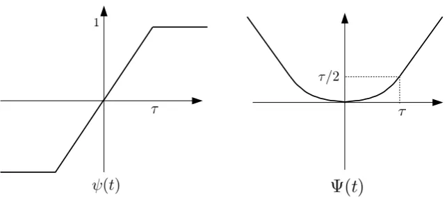
Without loss of generality, we take s= 0. Now consider the tent map and its integral as follows
φ(t) =
(
1− |t|/τ for|t|< τ
0 otherwise
Φ(t) =
Z t
0
φ(t) =
(
t−sgn(t)2t2τ for|t|< τ sgn(t)τ2 otherwise
For a sketch of φand Φ see figure 2.1. Let ζ = Φxand η = φx, then differ-entiation ζ with respect to time we have ˙ζ =A(t)ζ+η. By the definition of uniform hyperbolicity there is a unique bounded solution β=L−1η. Now let
x+= (β−ζ)/τ+
1 2x
x−= (β−ζ)/τ− 1
2x (2.11)
and note thatx+ satisfies ˙x+ =Ax+ and equalsβ/τ fort > τ, so is bounded
Figure 2.2: A sketch showing the vector spaces E±(s) as the range of the re-spective projections P±(s) varying through time. The arrows from the origin at times onE±(s) indicate the respective vector space contracts forward and backward in time respectively. Also shown, at times, the pointxis projected tox±(s) byP±(s) respectively.
By construction, since L−1 is linear, P
± are linear and sum to the identity. The ranges of P± have intersection {0} since the free linear system has no non–trivial bounded solution on the whole of R. To see they are projections,
take P+x0 = x+(0) as new initial condition and define η+, ζ+, β+ to be the
corresponding functions above. Then (β+−ζ+)/τ−12x+is bounded not only for
t <0 but also fort >0 since each of its terms is bounded fort >0. But the free linear system has no non–trivial bounded solution, thus (β+−ζ+)/τ−12x+= 0,
i.e. P−P+x0 = 0. From P++P− =I we deduce that P±2 = P±. To obtain uniform bounds forP±, note that from the choice ofτ,|x(t)| ≤e|t|/τ|x0|,
|β(0)| ≤ |β|0≤ |β|1≤K−1|η|0=K−1 sup
|t|<τ
(1−|t|
τ)|x(t)| ≤K
−1
|x0| (2.12)
since (1−|τt|)e|t|/τ is a decreasing function of|t|. Also notingζ(0) = 0 we have
|x+(0)|=|(β(0)−ζ(0))/τ+
1
2x(0)| ≤( 1
Kτ +
1
2)|x0| (2.13) Thus|P+| ≤Kτ1 +21 and similarly|P−| ≤τ K1 +
1 2.
Figure 2.3: A sketch of the “switch” mapψand its integral Ψ.
are bounded while the backward orbits fromR( ˜P−(t)) are bounded. The latter condition determinesP±(t) uniquely, soP±(t) = ˜P±(t). Hence, the invariance conditionP±(t)X(t,0) =X(t,0)P±(0).
Obtaining C(µ, τ)
To obtain the exponentially decaying bounds forx±we make use of the “switch” map and its integral, see figure 2.3 for a sketch,
ψ(t) =
( t
τ for|t|< τ
sign(t) otherwise
Ψ(t) =
Z t
0
ψ(u)du=
( t2
2τ for|t|< τ |t| −τ
2 otherwise.
(2.14)
Consider the following perturbed linear operator
Lµ:C1→C0 (2.15)
ζ7→ζ˙−Aζ−µψζ.
Forµ∈[0, K),Lµ is invertible with||Lµ−1||−1≥K−µ(applying Lemma 2.2.1
|A| ≤1/τ.We have
|η˜|0≤ sup
|t|<τ
|φ(t)x(t)eµΨ(t)|= sup |t|<τ
(1− |t|/τ)|x0|e
|t|
τ e t2 2τ2 ≤ |x
0| (2.17)
since (1− |t|/τ)e|τt|e t2
2τ2 is a decreasing function of |t|. But ˜η(0) =x0, so we
have the required equality. Then|β˜|1≤K1−µ|x0|and so
|β(t)| ≤ 1
K−µ|x0|e
−µΨ(t). (2.18)
Now ifx0∈ R(P+) thenx+=βτ + (12−Φτ)x+, so
x+=
β
Φ +τ /2 (2.19) and thus
|x+(t)| ≤
e−µΨ|x 0|
(K−µ)(Φ +τ /2). (2.20) So
|x+(t)| ≤C0(t)e−µt|x0|withC0(t) =
eµ(t−Ψ)
(K−µ)(Φ +τ /2). (2.21) Fort≥0,t−Ψ(t) = Φ(t) andC0 is non–increasing so we have the bound
C(µ, τ)≤ 2
(K−µ)τ fort≥0. (2.22)
Proceed similarly forx0∈ R(P−) and negative time. Note that this bound can be improved to
C(µ, τ)≤ e µτ /2
(K−µ)τ fort≥τ. (2.23)
Remarks 1
(i) One can optimise the decay estimate (2.21) over µ by using the bound (2.23). The optimum over µ is at µ = K − 1
t−τ /2 which is valid for
t≥ 3
2K if we setτ >1/K. Then the following bound can be obtained |x+(t)| ≤(
t τ −
1 2)e
1−K(t−τ /2)|x
0|fort≥
3
(ii) The functionsφandψcould be chosen asymmetrically, and different val-ues ofµcould be used for positive and negative time; if the resulting oper-ator (call itLµ+,µ−) happens to remain invertible for larger values of one
or both of µ± then stronger decay estimates follow. In particular, in the
attracting case, P− = 0.
2.3.2
Green functions and bounds on response for certain
types of forcing
The following definition can be found in (Cop78).
Definition 2.3.3 The Green’s function for a uniformly hyperbolic linear system is the matrix onR2 defined by
G(t, s) =
(
X(t, s)P+(s) fors < t −X(t, s)P−(s) fort < s.
Fixing s,G(t, s) is the unique bounded solution of ˙x(t) =A(t)x(t) fort6=swith
G(s+, s)−G(s−, s) =I. Note that by invariance of the projections,G(t, s) can also be written as
G(t, s) =
(
P+(t)X(t, s) fors < t −P−(t)X(t, s) fort < s
and that ∂2G(t, s) =−G(t, s)A(s) fors6=t,
G(t, t+)−G(t, t−) =I (2.25)
Theorem 2.3.2 If the linear system (2.3) is uniformly hyperbolic then it has the following properties.
(i) The unique bounded responsex=L−1[f]of (2.6) to the forcing,f, can be written as
x(t) =
Z +∞
−∞
G(t, s)f(s)ds. (2.26)
(ii) For anyµ∈[0, K)there exists D(µ)such that |G(t, s)| ≤De−µ|t−s|. (iii) If|f(s)| ≤εeµ|s| for someµ∈[0, K)then |x(t)| ≤ εeµ|t|
Proof:
(i) We can verify this by differentiating (2.26) w.r.t. t, taking care to first split the integral ats=twhere the integral is not differentiable:
˙
x(t) =
Z +∞
−∞
A(t)G(t, s)f(s)ds+P+(t)f(t) +P−(t)f(t)
=A(t)x(t) +f(t). (2.28)
ButL−1[f] is the unique bounded solution of ˙x=Ax+f, thus it is given
by (2.26).
(ii) A bound on |G(t, s)| can already be obtained by composition of those of the previous theorem for the projections and the evolution of vectors
in their ranges, but it will be useful to sharpen the estimate as follows. Repeat the estimates usingLµ as in the proof of the previous theorem to
obtain (2.18). Thenx+ =βτ + (12−Φτ)ximplies
eµt|x+(t)| ≤
eµ(t−Ψ(t))
τ(K−µ)+ ( 1 2−
Φ(t)
τ )e
µtet/τ
|x0|fort≥0. (2.29)
Note that for t ≥ 0, t−Ψ(t) attains its sup value of τ2 at t ≥τ; (12 − Φ(t)
τ )e (µ+1
τ)t attains its sup value of 1
2 at t = 0 since it is a decreasing
function on t≥0. Thus
|x+(t)| ≤De−µt|x0| (2.30)
for t≥0 withD = eµτ /2 (K−µ)τ +
1
2. Similarly |x−(t)| ≤De
−µt|x
0|for t≤0.
This result could be optimised over µif desired.
(iii) If|f(s)| ≤εeµ|s|then Lx=f is equivalent toL
−µx˜= ˜f with ˜x=e−µΨx
and ˜f =e−µΨf, whereL−µ is as defined in (2.15) but using the opposite
sign of µ and Ψ is as defined in (2.14) except now we allow its value of
τ to differ from that in the definition of the norm | · |1 in (2.8). Then ||L−−1µ||−1≥K−µforµ∈[0, K), so
|x˜| ≤ |f˜|
K−µ. (2.31)
This gives
|x(t)e−µΨ(t)|=|x˜(t)| ≤ |f˜|
K−µ ≤ ε
K−µ. (2.32)
(iv) If f is a bounded function with f(s) = 0 for all s∈(−T, T) then again (2.31) with τ→0 gives
|x(t)| ≤ e
−µ(T−|t|)|f|
K−µ . (2.33)
The minimum over µ∈ [0, K) is achieved at µ=K− 1
|t|−T which is in
[0, K) for|t| ≤T−1/K, giving the optimised result.
Theorem 2.3.3 If 0 ≤ α < K ≤ ||L−1||−1, |f(s)| ≤ F, |f(s)| ≤ εeα|s| for
s∈(−T, T),x=L−1[f],|t| ≤T −1/K, then
|x(t)| ≤ ε
K−αe
α|t|+ (T− |t|)e1−K(T−|t|)F. (2.34)
Proof: Consider
f1(t) =
f(t) for|t|< T
(t+T+ 1)f(−T) for−T−1< t <−T
(T+ 1−t)f(T) forT < t < T + 1 0 for|t|> T+ 1 and
f2(t) =
0 for|t|< T
f(t)−(t+T + 1)f(−T) for−T−1< t <−T f(t)−(T+ 1−t)f(T) forT < t < T+ 1
f(t) for|t|> T+ 1.
Note thatf =f1+f2, so we have
|x(t)| ≤ |L−1[f1](t)|+|L−1[f2](t)| (2.35)
By Theorem 2.3.2 (iii) and (iv), we have|L−1[f1](t)| ≤ εe
α|t|
K−α and|L
−1[f 2](t)| ≤
(T− |t|)e1−K(T−|t|)F for|t| ≤T −1/K. Adding the two gives the result.
The use of this result is to suppose that εis small and that we can take T =
1 γlog
F
ε for some γ ∈ (α, K). Then roughly speaking the first term of (2.34)
Hence|x(t)| ≤ ε+KO−(αε)eα|t|, uniformly on any bounded interval oft.
Proof: Consider the ratioρ=ye1−yxof the second term of (2.34) to the first where y= (K−α)(T− |t|) andx= εeFαT. So ρ≤1 wheny≥g(x) where g is
the inverse function toey−1/yony≥1.
We will show thatg is bounded above by the function ¯g(x) = log(2exlog(ex)). Consider the equationx=ey−1/ywhich, after some manipulation, gives
log(2ex(logxe)) =y+ log(2(1−logyy)). But logyy has maximum aty=e1 with largest valuee−1, so 2(1−logy
y )≥1 giving us ¯g≥g.
So y ≥ ¯g(x) implies the second term (2.34) is at most the first. Now logx= logFε −αT = (γ −α)T if we take T = γ1logFε with γ ∈ (α, K). Thus the second term is at most the first when y ≥ logx+ log(2e(1 + logx)) i.e (K−α)(T− |t|)≥(γ−α)T+ log(2e(1 + (γ−α)T)) which gives
|t| ≤T− 1
K−α((γ−α)T + log(2e(1 + (γ−α)T)))
≤K−γ
K−αT −
1
K−αlog(2e(1 + (γ−α)T)). (2.36)
Similarly, for anyp >0, we obtainρ≤pify≥g(x/p), which is true if
|t| ≤ K−γ
K−αT −
1
K−αlog(
2e
p(1 + (γ−α)T) + log(1/p)).
≤ K−γ
K−αT. (2.37)
2.3.3
Continuity of the splitting
Let F be a uniformly hyperbolic set, then it can be useful to know how the
projections P±(t) vary across the members of the set. With some Lipschitz conditions on how the set is generated it can be shown that the projections vary
H¨older continuously. This is stated more precisely in the following theorem.
Definition 2.3.4 Let A be a matrix function evaluated on the time–extended state space. Take F to be the set of those matrix functions that are given by
A(t) =A(y(t), t)wherey(·)is an orbit of some vector fieldy˙=u(y, t). We say
F is generated byA andu.
Theorem 2.3.4 Assume A(bounded) anduare Lipschitz and let F be a uni-formly hyperbolic set generated by A and u, then the projections P±(t) vary
The difficulty here is that the trajectories from nearbyy0att= 0 may separate
arbitrarily far and the bound
|∆A| ≤Var(A) = sup
y1,y2,t
|A(y1, t)− A(y2, t)| (2.38)
is in general insufficient to apply the perturbation Lemma 2.2.1 and in any case
is insensitive to|∆y0|. Thus we will need to work harder.
Before we state the proof, we note one simple consequence of the continuity of P± in the finite-dimensional case – their ranks are constant on connected components, which can be easily argued by contradiction: Let P and P0 be projections based aty0 andy00 respectively where|y0−y00|is arbitrarily small.
AssumeP0has greater rank thanP, then by counting dimensionsN(P)∩R(P0) is non–trivial. Thus it contains a non-zerov that satisfiesP v= 0 andP0v=v, so|P−P0| ≥1, which contradicts continuity.
Proof: Unless stated otherwise, all integrals are definite integrals overR. First,
we note the difference between the inverses of two invertible linear operators is
given by
L−11−L−01=L1−1(L0−L1)L−01. (2.39)
In our case L0−L1= ∆A=A1−A0, so if we denote ∆G(t, u) :=G1(t, u)−
G0(t, u), we have
Z
∆G(t, u)f(u)du=(L1−1−L−01)[f](t)
=
Z
G1(t, s)∆A(s)
Z
G0(s, u)f(u)du
ds
=
Z Z
G1(t, s)∆A(s)G0(s, u)ds
f(u)du
(2.40)
which gives
∆G(t, u) =
Z
G1(t, s)∆A(s)G0(s, u)ds.
estimate|∆y(t)| ≤eλ|t||∆y
0|, so|∆A(t)| ≤αeλ|t||∆y0|.
Using the estimate of|G(t, s)| ≤De−µ|t−s|of Theorem 2.3.2 (ii) we obtain
|∆P+(t)| ≤
Z
D2e−2µ|t−s|min{αeλ|s||∆y0|, V}ds. (2.42)
Supposing |∆y0| ≤ V /α, let s∗ ≥ 0 be the value such that αeλs
∗
|∆y0| = V,
so eλs∗ = α|∆Vy
0|. Taking |∆y0| small enough so that −s
∗ < t and assuming without loss of generality thatt <0,
|∆P+(t)| ≤
Z −s∗
−∞
D2V e−2µ|s−t|ds+
Z t
−s∗ +
Z 0
t
+
Z s∗
0
D2e−2µ|s−t|αeλ|s||∆y0|ds
+
Z ∞
s∗
D2V e−2µ|s−t|ds. (2.43)
[image:25.595.184.524.469.666.2]See Figure 2.4 for a sketch of the exponential bounds and the five regions of
integration. Puttingξ=α|∆y(0)|/V ≤1, each integral evaluates as follows
1stintegral ≤
Z −s∗
−∞
V D2e2µ(s−t)ds
≤V D
2
2µ e
2µ(s∗−t)
≤V D
2
2µ e
2µ|t|ξ2µ/λ,
2ndintegral ≤
Z t
−s∗
V D2ξe(2µ−λ)s−λtds
≤ V D
2
2µ−λξ
eλ|t|−ξ2µ/λe2µλ|t|ξ−1
≤ V D
2
2µ−λe
λ|t|
ξ−ξ2µ/λe(2µ−λ)|t|
,
Note that ifλ= 2µthis term is interpreted as V Dλ2e−2µtξlogξ−1.
3rd integral ≤
Z 0
t
V D2ξe−2µ(s−t)e−λtds
≤ V D
2
−2µ−λξ
e2µt−e−λt
,
4thintegral ≤
Z s∗
0
V D2e−2µ(s−t)eλtds
≤ V D
2
2µ−λe
−2µ|t|ξ−ξ2µ/λ
≤ V D
2
2µ−λe
−2µ|t|
ξ−ξ2µ/λe4µ|t|
,
5thintegral ≤
Z ∞
s∗
V D2e−2µ(s−t)ds
≤V D
2
2µ e
−2µ|t|ξ2µ/λ.
Thus for small enough |∆y0| we have |∆P+(t)| = O(|∆y0|δ) for some 0 < δ
(although not uniformly overt) henceP+ is H¨older continuous with respect to
as follows:
1st+ 5thintegral ≤ V D 2
µ e
2µ|t|ξ2µ/λ
2nd+ 4thintegral ≤ V D 2
2µ−λ
eλ|t|+e−2µ|t|
ξ− 2V D 2
2µ−λe
2µ|t|ξ2µ/λ. (2.44)
So the sum of all four integral is bounded by
1st+ 5th+ 2nd+ 4th≤ V D 2
2µ−λ
eλ|t|+e−2µ|t|
ξ+
V D2
µ −
2V D2
2µ−λ
e2µ|t|ξ2µ/λ
≤ V D
2
2µ−λ
eλ|t|+e−2µ|t|
ξ− λV D 2
2µ−λe
2µ|t|ξ2µ/λ
≤ V D
2
2µ−λ
eλ|t|+e−2µ|t|
ξ. (2.45)
Adding the bound for the 3rd integral we have |∆P+(t)| = O(ξ) = O(|∆y0|)
henceP+ is Lipschitz with respect toy0.
The same applies toP−.
At a later stage we will consider a perturbed set ˜F generated by A and ˜u, a perturbation ofu. It will be useful to know that the Green’s function resulting from a concatenation of truncated orbits of the perturbed and unperturbed
systems also varies H¨older continuously. The specific choice will be given on the next page. For now, take a trajectory ˜y(·) of the perturbed system ˙y= ˜u(y, t) and consider the unperturbed trajectory y(·) that passes through (˜y(σ), σ) for someσ. First we calculate a timeS that |∆A(t)|=|A(˜y(t), t)− A(y(t), t)| ≤η
remains true for|t−σ| ≤S for some η (we will truncate ˜y atσ±S). Now the difference ∆y(t) between the perturbed and unperturbed trajectory starting at (˜y(σ), σ) evolves by
∆ ˙y= ˜u(˜y, t)−u(y, t) = ∆u(˜y, t) + (u(˜y, t)−u(y, t)) (2.46)
starting from ∆y(σ) = 0. The second term is at most λ∆y(t) where λ is the Lipschitz constant ofu, so we have the Gronwall’s estimate
|∆y(t)| ≤
Z t
σ
dseλ|s−σ||∆u(˜y(s), s)|
≤e
λ|t−σ|−1
λ |∆u|
≤e
λ|t−σ|
Taking Lipschitz constantαforAwe obtain
|∆A(t)| ≤α|∆y(t)| ≤ α
λe
λ|t−σ||∆u|. (2.48)
Thus|∆A(t)| ≤η for all|t−σ| ≤S if
e−λS = α
λ
|∆u|
η . (2.49)
The choice ofη determines how big the perturbation|∆u| can be.
We are now ready to define, for anyσ, a concatenated path as follows
yσ(t) =
˜
y(t) for|t−σ| ≤S y(t) for|t−σ| ≥S+ε0
yσ−(t) forσ−S−ε0< t < σ−S
yσ
+(t) forσ+S < t < σ+S+ε0
wherey is the unperturbed trajectory passing through (˜y(σ), σ),
yσ
−(t) =τ−σ(t)˜y(σ−S) + (1−τ−σ(t))y(σ−S−ε0) and
yσ
+(t) =τ+σ(t)˜y(σ+S) + (1−τ+σ(t))y(σ+S+ε0) withτ−σ :t7→
t−(σ−S−ε0)
ε0 and
τ+σ :t7→
t−(σ+S)
ε0 . Soy
σ is essentially a concatenation of truncation of ˜y andy
withyσ
− andy+σ (see Figure 2.5). Note that ε0 can be chosen to be as small as
[image:28.595.185.516.474.668.2]Corollary 2.3.2 AssumeL:x7→x˙− A(y(t), t)xhas bound||L−1||−1≥Kand
letη < K/2. Fixε0≤η/(α|u|)whereα= LipyAand consider the following set
of operators parametrised by σ
Lσ:C1→C0
x7→x˙−Aσ(t)x (2.50)
with Aσ(t) =A(yσ(t), t). ThenLσ is invertible and the Green’s function Gσ is
continuous with respect toσ.
Proof: Unless stated otherwise, all integrals are definite integrals over R. Lσ
is invertible since it can be shown to be just a small perturbation ofL. Firstly, we show that|∆A(t)|:=|A(yσ(t), t)− A(y(t), t)| ≤2ηfor allt.
It is clear that|∆A(t)|= 0 for|t−σ| ≥S+ε0 and from howS was calculated
we see that|∆A(t)| ≤ηfor|t−σ| ≤S.
Now forσ−S−ε0< t < σ−S we have
|∆A(t)| ≤α|y−(t)−y(t)|=α|τ−σ(t)(˜y(σ−S)−y(σ−S−ε0))| ≤α|y˜(σ−S)−y(σ−S−ε0))|
≤α|y˜(σ−S)−y(σ−S))|+α|y(σ−S)−y(σ−S−ε0)|
≤αe
−λS
λ |∆u|+α|u|ε0≤η+η
≤2η. (2.51)
Similarly forσ+S < t < σ+S+ε0we have|∆A(t)| ≤2η. Note thatε0can be
chosen very small so that better bounds can be obtained, i.e. |∆A| ≤(1 +ε)η
for some smallε.
So Lσ is a perturbation of L with ||∆L|| = |∆A| ≤ 2η. By Lemma 2.2.1, if
2η < KthenLσ is invertible with bound
||L−σ1||−1≥K−2η. (2.52)
To show the Green’s function Gσ is continuous with respect toσwe prove the
projectionsPσ
± are continuous with respect toσ. Let us assume without loss of generalityσ0 < σ= 0. Now consideryσ0 which is a concatenation of truncations of ˜yandy0withyσ0
+ andyσ
0
Figure 2.6: A sketch ofyσ0 andyσ
|∆Aσ|=|Aσ−Aσ0|then just as in expression (2.41) we have
∆P+σ(t) =
Z
Gσ(t+, s)∆Aσ(s)Gσ0(s, t)ds. (2.53)
We see that ∆Aσ(s) = ∆A(s) := A(y(s), s)− A(y0(s), s) fors < σ0−S−ε0
and s > S+ε0 and ∆Aσ(s) = 0 for−S < s < S+σ0. Using the estimate of |Gx(t, s)| ≤De−µ|t−s|of Theorem 2.3.2 (ii) wherex=σ, σ0 andµ∈[0, K−2η)
we have the following bound
|∆P+σ(t)| ≤
Z
D2e−2µ|t−s||∆A(s)|ds+
Z −S
σ0−S−ε
0
+
Z S+σ0
S+ε0
D2e−2µ|t−s||∆Aσ(s)|ds.
(2.54)
We show that each integral isO(|∆σ|δ) =O(|σ0|δ) for some 0< δwhich implies
H¨older continuity. From the bound in (2.42) we saw the 1stintegral isO(|∆y 0|δ).
But |∆y0| = |y(0)−y0(0)| ≤ |y(0)−y˜(σ0)|+|y˜(σ0)−y0(0)| ≤ |u˜||σ0|+|u||σ0|
henceO(|∆y0|δ) =O(|∆σ|δ). Now let us treat the 2nd integral (by symmetry
the 3rd is the same), which can be further split into 3 integrals
we first show|∆Aσ(s)|=O(|σ0|) fors∈[−S−ε0, σ0−S] as follows
|∆Aσ(s)| ≤α|y−σ(s)−y
σ0
−(s)|
≤ατ−σ(s)˜y(−S)−τσ
0
−(s)˜y(σ0−S) + (1−τ−σ(s))y(−S−ε0)−(1−τσ
0
−(s))y0(σ0−S−ε0)
≤α σ0 ε0 ˜
y(σ0−S)−y0(σ0−S−ε0)
+τ−σ(s)
˜
y(−S)−y˜(σ0−S)
+ (1−τ−σ(s))
y(−S−ε0)−y0(σ0−S−ε0)
≤α ε0
|y˜(σ0−S)−y0(σ0−S−ε0)||σ0|+α|y˜(−S)−y˜(σ0−S)|
+α|y(−S−ε0)−y0(σ0−S−ε0)|. (2.56)
We can see the first term isO(|σ0|) and the second term is bounded byα|σ0||u˜|
hence is alsoO(|σ0|). Now for the third term
3rd term ≤α|y(−S−ε0)−y0(−S−ε0) +y0(−S−ε0)−y0(σ0−S−ε0)| ≤αy(0)−y
0(0)
λ e
λ|S+ε0|+α|σ0||u|
≤α(|u|+|u
0|)|σ0|
λ e
λ|S+ε0|+α|σ0||u|, (2.57)
hence it is also O(|σ0|). Thus the second integral of (2.55) is O(|σ0|) as it is an integral of anO(|σ0|) function over a finite range. So the second integral of (2.54) isO(|σ0|). From this we can conclude that|∆P+σ(t)|=O(|σ0|δ) for some
0 < δ although not uniformly over t. This implies Pσ
+ and hence Gσ, varies
H¨older continuously with respect toσ.
2.3.4
Set of uniformly hyperbolic systems and pseudo–
orbits
Given a uniformly hyperbolic set F that is generated by Aand u, it is useful to know if the set ˜F generated by perturbing uremains uniformly hyperbolic. This proves to be true for small enough perturbations as we shall see in the
following theorem.
Theorem 2.3.5 Let A(bounded) and ube Lipschitz and letF be a uniformly hyperbolic set with bound K that is generated by A and u. Let u˜ be a pertur-bation. If |∆u| = |u˜−u|0 is small enough, the set F˜ generated by A and u˜
In other words, given the assumptions of the above theorem there is a ˜K
such that for all orbits ˜y(·) of ˙y = ˜u(˜y, t), the linear operator ˜L associated to ˜A(t) =A(˜y(t), t) is invertible and it satisfies the bound||L˜−1||−1≥K˜.
There are various approaches to show the invertibility of ˜L. A nice one which is similar to (Pal00), involves constructing approximate right and left inverses
T and U in the sense that ||I−LT˜ || =εT < 1,||I−UL˜|| =εU <1, so that
˜
LT andUL˜ are invertible with norms at most 1/(1−εT) and 1/(1−εU). Then
T( ˜LT)−1 is a true right inverse to ˜L and (UL˜)−1U is a true left inverse, so
˜
L is invertible. Finally, one should show that T or U is bounded and then
||L˜−1|| ≤ ||T||/(1−ε
T) or≤ ||U||/(1−εU).
Even with this approach there are various possible choices for the approximate
inverses. The difficulty is in constructing the left inverse since UL˜ is a map-ping from C1 to C1 so the derivative has to be estimated too. We will give a
construction whereT =U.
Proof: Take
T[f](t) =
Z
ds1
2a
Z t+a
t−a
dσ Gσ(t, s)f(s) (2.58)
where Gσ is the Green’s function for Lσx(t) = ˙x(t)−Aσ(t)x(t) withAσ(t) = A(yσ(t), t) and yσ(t) is a concatenation of paths as given in (2.3.3), and a is
some duration of order τ. Note that it makes sense to integrate Gσ over σ
because by corollary 2.3.2 it depends continuously onσ.
Bounding ||T||
We treat T as an operator from C0 to C1 and wish to bound it. For each σ,
R
ds Gσ(t, s)f(s)≤ |f|/(K−2η) because, as we saw in corollary 2.3.2,A was
changed by at most 2η along an unperturbed trajectory. Thus averaging over an interval ofσproduces|T[f](t)| ≤ |f|/(K−2η).
Now we bound the derivative. To take care of the jump in Gσ(t, s) at s =t,
we writeT[f](t) = (R−∞t +Rt∞)ds 21aRtt−+aadσ Gσ(t, s)f(s) and now differentiate
with respect to tto obtain
τ ∂t(T[f])(t) =
τ
2a
Z
Note interchanges of order of integration and differentiation under the
inte-gral sign and with respect to limits are all valid.
To bound the first integral in (2.59), we use the same idea as in the proof of continuity of the splitting
Z
∆G(t, s)f(s)ds=
Z
dr Gt+a(t, r)∆A(r)
Z
ds Gt−a(r, s)f(s). (2.60)
Now|R
ds Gt−a(r, s)f(s)| ≤ |f|/(K−2η),|∆A| ≤V and ∆A(r) = 0 for|r−t| ≤
S−awhere S = −λ1log(α|λη∆u|) as in (2.49), so applying Theorem 2.3.2(iv) we obtain
|
Z
∆G(t, s)f(s)| ≤ε|f|/(K−2η) (2.61)
where
ε= (S−a)e1−(K−2η)(S−a)V (2.62)
provided (K−2η)(S−a)≥1, which is true if ∆uis small enough.
Combining the bounds for the two terms of (2.59), we obtain
τ|∂t(T[f])(t)| ≤(1 +
τ
2aε)|f|/(K−2η). (2.63)
So we obtain
||T|| ≤(1 + τ
2aε)/(K−2η), (2.64)
which is only slightly larger than K−1. To optimise the result, it is useful to chooseη to depend on|∆u|in such a way as to make the corrections in the nu-merator and denominator of roughly equal relative size. This is achieved approx-imately by takingη ∝ |∆u|K/(K+λ). More specifically (2.62) saysε≈V e−KS
(on a logarithmic scale of approximation), so ε2τa = η/K if η ≈ KV 2τae−KS.
But (2.49) says η = α λ|∆u|e
λS so eliminating S between these two equations
yields
η ≈
KV τ
2a
K+λλ α
λ|∆u|
K+λK
Estimating I−LT˜
This is an operator fromC0 toC0.
(I−LT˜ )[f](t) =f(t)−(∂t−A˜(t))(
Z t
−∞ +
Z ∞
t
)ds 1
2a
Z t+a
t−a
dσ Gσ(t, s)f(s).
(2.66)
This evaluates to
−1
2a
Z
ds∆G(t, s)f(s) + 1 2a
Z
dσ
Z
ds∆Aσ(t)Gσ(t, s)f(s). (2.67)
But|∆Aσ(t)|=|A˜(t)−Aσ(t)|= 0 for|t−σ| ≤S, so taking|∆u|small enough
thatS > a, we have only the first term, which we bounded in (2.61), so
||I−LT˜ || ≤ ε
2a(K−2η). (2.68)
So if ε <2aK, T is an approximate right inverse of ˜L forη small enough and ( ˜LT)−1 exists. ThenT( ˜LT)−1is a true right inverse of ˜L.
Estimating I−TL˜
This is an operator from C1 to C1 so we have to bound both its value acting
on anyC1functionxand the value of its derivative.
(I−TL˜)[x](t) =x(t)− 1
2a
Z t+a
t−a
dσ( Z t −∞ + Z ∞ t
)ds Gσ(t, s)(∂s−A˜(s))x(s).
(2.69)
Integrating by parts and using∂sGσ(t, s) =−Gσ(t, s)Aσ(s)−Iδ(t−s) (where
the use of Dirac δ–function is a convenient encoding of the jump condition (2.25)) transforms this to
1 2a
Z
dσ
Z
ds Gσ(t, s)∆Aσ(s)x(s), (2.70)
and ∆Aσ(s) = 0 for|s−σ| ≤S, hence for|s−t| ≤S−a, so it can be bounded
Next we bound the derivative of (2.70).
∂t
1 2a
Z t+a
t−a
dσ( Z t −∞ + Z ∞ t
)ds Gσ(t, s)∆Aσ(s)x(s) =
1 2a
Z
(Gt+a(t, s)∆At+a(s)−Gt−a(t, s)∆At−a(s))x(s)ds
+ 1 2a
Z
(Gσ(t, t−)−Gσ(t, t+))∆Aσ(t)x(t)dσ
+ 1 2a
Z Z
Aσ(t)Gσ(t, s)∆Aσ(s)x(s)dsdσ. (2.71)
The second term is zero because ∆Aσ(t) = 0 forσ∈(t−a, t+a). The third
term has ∆Aσ(s) = 0 for|s−t| ≤S−a, so is bounded byε|A||x|. Similarly,
each term of the first integral is bounded by 2εa|x|. Thus
τ|∂t(I−TL˜)[x](t)| ≤(
τ
a+τ|A|)ε|x|. (2.72)
Finally we can chooseτ < aandτ|A| ≤1, so we obtain
||I−TL˜|| ≤2ε. (2.73)
So ifε <1/2,T is an approximate right inverse of ˜Land (TL˜)−1 exists. Then (TL˜)−1T a true left inverse of ˜L.
Obtaining K˜
Thus if ε =V(S−a)e1−(K−2η)(S−a) <min(1
2, 2aK) we have both ||I−LT˜ ||
and||I−TL˜||<1, so ˜Lis invertible. From (2.64) and (2.73) we have the bound
||L˜−1||−1≥ (1−2ε)(K−2η)
1 +ε/2 = ˜K. (2.74) Choosingη∝ |∆u|K/(K+λ) we obtain
||L˜−1||−1≥K−O(|∆u|K/(K+λ)) (2.75)
which says that ˜K is slightly smaller thanKfor ∆usmall.
Constructing the Green’s function G˜
Now that we know the pseudo–orbit ˜y is uniformly hyperbolic, one can con-struct its true Green’s function ˜G using the unperturbed set F. For each time s, consider y(·) that solves the unperturbed equation ˙y = u(y, t) start-ing at y(s) = ˜y(s) and letE±(·) be the exponential dichotomy splitting along
y(·). Let ˜X be the principal matrix solution of ˙x= ˜A(t)x, take the subspace ˜
similarly ˜E+(t) = lims→+∞X˜(t, s)E+(s). Then construct complementary
Chapter 3
Invariant manifolds and
normal hyperbolicity
3.1
Normal hyperbolicity and invariant
mani-folds
The concept of normal hyperbolicity applies to the context of nonlinear systems that have some invariant manifold, M, in which any tangential contraction
in forward or backward time is weaker than any transverse contraction in the same direction of time. The definition is a local statement at M, thus the
linearised dynamic at M is central to the study. As such, when considering continuous–time dynamics normal hyperbolicity theory can employ the results
from Chapter 2 on uniform hyperbolicity. In particular, the transverse linearised dynamic along the set of trajectories on M generates a uniformly hyperbolic
set. Thus the theory on C1 perturbation of the nonlinear system can make
use of the result on pseudo–orbits in section 2.3.4 of Chapter 2. In the context
of non–autonomous systems, M is non–compact as it is defined on the time– extended space.
In (Fen71), the unperturbed invariant manifold M is assumed compact and
if it has a boundary it is taken to be “invariant overflowing” which means the backward orbits remain in the manifold and the vector field through any
point on the boundary is strictly outward pointing. Under certain conditions
on the generalised Lyapunov type numbers for the flow,M persists under any small perturbation of the system. The perturbed invariant manifold ¯M arises
from the fixed point of a graph transform G which acts on a space of Lips-chitz graphs from a reference manifold (e.g. unperturbed M) to a transverse
which loosely speaking, takes each point on a candidate graph, computes their pre–image along the tangential direction on the candidate graph, then with this
pre–image, flow forward in the transverse direction to obtain a point which is taken to be the point on the iterated graph. If there is transverse expansion,
Gis defined by solving an implicit zero equation introduced by the expansion, and separately solving a standard graph transform equation.
The graph transform method is also used in (HPS77) in discrete–time setting where the non–compact case was also dealt with (Theorem (6.1) in (HPS77)).
The definition of normal hyperbolicity in (HPS77) is given by spectral gap con-ditions that reflect the dominance of the transverse contraction or expansion
rates over those in the tangential direction– which is another way of expressing the generalised Lyapunov type numbers in (Fen71). If the unperturbed discrete
mapf has no transverse expansion the treatment is identical to (Fen71). How-ever, if there were transverse expansion, the local unstable manifold Wu
¯ f( ¯M)
of the perturbed invariant manifold ¯Munder the perturbed map ¯f is given by the fixed point of the standard graph transform Gs defined as in (Fen71). Gs
has contraction rate roughly equal to the ratio of the transverse contraction rate and the tangential contraction rate off. SimilarlyWs
¯
f( ¯M) is constructed
by applying the previous step to ¯f−1 with a graph transform Gu which has contraction rate roughly equal to the ratio of the transverse expansion rate and
the tangential expansion rate off. Then ¯Mis found by taking the intersection
Ws ¯
f( ¯M)∩W s ¯ f( ¯M).
We introduce the definition of normal hyperbolicity in our context and show
that the standard definition implies it. We note that the definition given here is more general in the sense that it allows the hyperbolic rates to vary with
time. We will give a Theorem 3.2.2 based on Dan Henry (Hen81) that give the invariant manifold under certain conditions and assumptions. This is a path–
wise approach which is advantageous as it avoids the graph transform. The proof of the C1 property and the normal hyperbolicity of this invariant
man-ifold is for future development. A second approach outlined here is given in Conjecture 1 which is a hybrid of path–wise and graph transform approach. A
brief description of the standard graph transform approach for computing the
invariant manifold will also be given in Theorem 3.2.3. A comparison between these approaches and recent work by (BOV97, GV04, BHV03) will be given at
Attention will be restricted to non–autonomous systems of the form
˙
θ= Θ(θ, r, t) ˙
r=R(θ, r, t) ˙
t= 1 (3.1)
withr∈Rnandθ∈M whereM is some compact submanifold without
bound-ary. In the application to a non–autonomous oscillator, M = R/TZ, which represents a limit cycle with period T. This product structure M ×Rn×R is
not a great restriction, as the normal bundle to a submanifold can always be
trivialised by adding some artificial extra dimensions to the fibres cf. (Eld12) section 2.5, 2.6 and references within.
3.2
Computing the invariant manifold
We wish to show that under certain conditions the non–autonomous system
(3.1) has a normally hyperbolic invariant submanifold.
Let us consider the space of Lipschitz graphs whose Lipschitz constant with respect to θis at mostl>0
G={ρ:M ×R→U |Lipθρ≤l} (3.2)
whereU ={r∈Rn||r| ≤ξ}.
Note that we use the term “graph” for an element ofρ∈ Ginterchangeably with the graph ofρgiven by graph(ρ) :={(θ, ρ(θ, t), t)∈M×U×R: (θ, t)∈M×R}.
A graph transform type approach requires the consideration of G which the graph transform acts on – this is considered in Conjecture 1. However, a path–
wise approach will be given based on (Hen81) in Theorem 3.2.2 which does not use a graph transform.
3.2.1
Two operators
We will consider two operators that are key to our study of invariant manifold.
The notation here is that the partial derivative of a vector fieldX with respect to x is written as Xx and the sup norm over the defining domain is simply
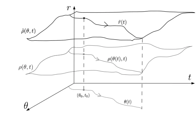
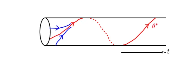
Definition 3.2.1 (Pseudo–orbit) Forρ∈ G and(θ0, t0)∈M ×R define the
corresponding pseudo orbitθρ,θ0,t0:R→M as the solution toθ˙= Θ(θ, ρ(θ, t), t)
starting atθ(t0) =θ0.
To simplify notation we drop the subscripts in θρ,θ0,t0(t).
Definition 3.2.2 (OperatorL) Forρ∈ G and(θ0, t0)∈M×R,consider the
corresponding pseudo–orbitθ(·). Then for anyC0 functionr:
R→U we define
the operator Lr:C1(R,Rn)→C0(R,Rn)by
Lr[x](t) = ˙x(t)−Rrx(t). (3.3)
with Rr evaluated onp(t) = (θ(t), r(t), t).
Note that the subscript inLr refers to the functionr(·).
Definition 3.2.3 (OperatorJ) Consider the definition of the operatorLabove. Given in addition aC0 function σ¯:
R→L(T M,Rn)we define
Jσ¯ :W1,∞(R, L(T M,Rn))→W0,∞(R, L(T M,Rn))by
Jσ¯[σ](t) = ˙σ−Rrσ+σ(Θθ+ Θrσ¯), (3.4)
withRr,Θθ,Θrevaluated onp(t)and whereW1,∞is the space of bounded
Lip-schitz functions and W0,∞ the space of L∞ functions.
We enlarge the natural Jσ¯ : C1 → C0 setting here to cater for some forcing
functions that will not be continuous e.g. arising from the discontinuity in the
Green’s function forL ats=t, or from our allowing Lipschitz graphs not just
C1 graphs. By Rademacher’s theorem, see (ACP10), any function σ ∈W1,∞ is differentiable almost everywhere. Thus we can equip W1,∞ with the norm
|σ|1,∞ = max{|σ|0, τ|σ˙|∞} where | · |∞ is the L∞ norm and τ chosen so that
τ|Rr|, τ|Θr|, τ|Θθ| ≤1.
Note thatJ¯σis related to the slope dynamic and in particular the Ricatti
equa-tion
˙
σ=Rθ+Rrσ−σ(Θθ+ Θrσ), (3.5)
Definition 3.2.4 (Set of pairs of operators) For anyρ∈ G, let us fixt0∈ Rand define the set of pairs of operatorsFρ:={(Lr, Jσ¯) :θ0∈M}where each
pair (Lr, Jσ¯) is defined given(θ0, t0)as above.
Definition 3.2.5 (Uniformly Hyperbolic set) Fρis a uniformly hyperbolic set with boundsK0 andκ0 if eachLr andJσ¯ are invertible with||L−r1||−1≥K0
and||J¯σ−1||−1≥κ0.
3.2.2
Definition of Normal Hyperbolicity
We give a definition of Normal Hyperbolicity using the two operators defined
above and show that the standard definition due to (HPS77) implies it.
Let F(t;p) be the flow of the non–autonomous system (3.1) starting at p ∈
M ×Rn×
Rwith end time t.
Definition 3.2.6 (Invariant graph) Consider ρ∈ G with M = graph(ρ) ∼=
M ×R. Then ρis an invariant graph under the non–autonomous system (3.1) if F(t;M) =M.
Ifρ∈ Gis invariant then for each (θ0, t0)∈M×R, lettingθbe the pseudo–orbit,
we taker(t) =ρ(θ(t), t) and ¯σ(t) =ρθ(θ(t), t) in the definition of Fρ.
Definition 3.2.7 (Normal Hyperbolicity with two operators) An invari-ant graphρ∈ G under the non–autonomous system (3.1) is normally hyperbolic iffFρ (using ¯σ=ρθ) is uniformly hyperbolic.
Compare this with the standard definition found in (HPS77):
Definition 3.2.8 (Standard definition of Normal Hyperbolicity) An in-variant graph ρ ∈ G under the non–autonomous system (3.1) is normally hy-perbolic iff the tangent bundle ofM×Rn×Rrestricted toM, splits into three
H¨older continuous subbundles
TM(M ×Rn×R) =V+⊕TM ⊕V− (3.6)
which are invariant by the linearised flow of F, denoted by DF, such that for allp0= (θ0, r0, t0)∈ M, t > t0,k∈ {0,1},
a) ||DF(t;p0)|V+(p0)|| ≤Cδ
|t−t0|[m(DF(t;p
0)|Tp0M)]
k (3.7)
and for allt < t0,k∈ {0,1},
b) ||DF(t;p0)|V−(p0)|| ≤Cδ
|t−t0|[m(DF(t;p
0)|Tp0M)]

![Figure 2.4: A sketch of e[−2µ|t−s| and min{eλ|s|, V } with t fixed and s varying.Note the five integration regions of (2.43) are [−∞, −s∗], [−s∗, t], [t, 0], [0, s∗] ands∗, ∞].](https://thumb-us.123doks.com/thumbv2/123dok_us/9647713.466918/25.595.184.524.469.666/figure-sketch-xed-varying-note-ve-integration-regions.webp)
![Figure 2.5: A sketch of yyσ(t) for the case σ = 0 which is a concatenation of y(t)for t ∈ [−∞, −(S + ε0)], yσ−(t) for t ∈ [−(S + ε0), −S], ˜y(t) and t ∈ [−S, S],σ+(t) for t ∈ [S, (S + ε0)] and y(t) for t ∈ [(S + ε0), ∞]](https://thumb-us.123doks.com/thumbv2/123dok_us/9647713.466918/28.595.185.516.474.668/figure-sketch-yys-case-concatenation-ys-e-e.webp)