University of Warwick institutional repository:
http://go.warwick.ac.uk/wrap
A Thesis Submitted for the Degree of PhD at the University of Warwick
http://go.warwick.ac.uk/wrap/56778
This thesis is made available online and is protected by original copyright.
Please scroll down to view the document itself.
Library Declaration and Deposit Agreement
1. STUDENT DETAILS
Please complete the following:
Full name: ………. University ID number: ………
2. THESIS DEPOSIT
2.1 I understand that under my registration at the University, I am required to deposit my thesis with the University in BOTH hard copy and in digital format. The digital version should normally be saved as a single pdf file.
2.2 The hard copy will be housed in the University Library. The digital version will be deposited in the University’s Institutional Repository (WRAP). Unless otherwise indicated (see 2.3 below) this will be made openly accessible on the Internet and will be supplied to the British Library to be made available online via its Electronic Theses Online Service (EThOS) service.
[At present, theses submitted for a Master’s degree by Research (MA, MSc, LLM, MS or MMedSci) are not being deposited in WRAP and not being made available via EthOS. This may change in future.]
2.3 In exceptional circumstances, the Chair of the Board of Graduate Studies may grant permission for an embargo to be placed on public access to the hard copy thesis for a limited period. It is also possible to apply separately for an embargo on the digital version. (Further information is available in the Guide to Examinations for Higher Degrees by Research.)
2.4 If you are depositing a thesis for a Master’s degree by Research, please complete section (a) below. For all other research degrees, please complete both sections (a) and (b) below:
(a) Hard Copy
I hereby deposit a hard copy of my thesis in the University Library to be made publicly available to readers (please delete as appropriate) EITHER immediately OR after an embargo period of ………... months/years as agreed by the Chair of the Board of Graduate Studies.
I agree that my thesis may be photocopied. YES / NO (Please delete as appropriate)
(b) Digital Copy
I hereby deposit a digital copy of my thesis to be held in WRAP and made available via EThOS.
Please choose one of the following options:
EITHER My thesis can be made publicly available online. YES / NO (Please delete as appropriate)
OR My thesis can be made publicly available only after…..[date] (Please give date)
YES / NO (Please delete as appropriate)
OR My full thesis cannot be made publicly available online but I am submitting a separately identified additional, abridged version that can be made available online.
YES / NO (Please delete as appropriate)
3. GRANTING OF NON-EXCLUSIVE RIGHTS
Whether I deposit my Work personally or through an assistant or other agent, I agree to the following:
Rights granted to the University of Warwick and the British Library and the user of the thesis through this agreement are non-exclusive. I retain all rights in the thesis in its present version or future versions. I agree that the institutional repository administrators and the British Library or their agents may, without changing content, digitise and migrate the thesis to any medium or format for the purpose of future preservation and accessibility.
4. DECLARATIONS
(a) I DECLARE THAT:
I am the author and owner of the copyright in the thesis and/or I have the authority of the authors and owners of the copyright in the thesis to make this agreement. Reproduction of any part of this thesis for teaching or in academic or other forms of publication is subject to the normal limitations on the use of copyrighted materials and to the proper and full acknowledgement of its source.
The digital version of the thesis I am supplying is the same version as the final, hard-bound copy submitted in completion of my degree, once any minor corrections have been completed.
I have exercised reasonable care to ensure that the thesis is original, and does not to the best of my knowledge break any UK law or other Intellectual Property Right, or contain any confidential material.
I understand that, through the medium of the Internet, files will be available to automated agents, and may be searched and copied by, for example, text mining and plagiarism detection software.
(b) IF I HAVE AGREED (in Section 2 above) TO MAKE MY THESIS PUBLICLY AVAILABLE DIGITALLY, I ALSO DECLARE THAT:
I grant the University of Warwick and the British Library a licence to make available on the Internet the thesis in digitised format through the Institutional Repository and through the British Library via the EThOS service.
If my thesis does include any substantial subsidiary material owned by third-party copyright holders, I have sought and obtained permission to include it in any version of my thesis available in digital format and that this permission encompasses the rights that I have granted to the University of Warwick and to the British Library.
5. LEGAL INFRINGEMENTS
I understand that neither the University of Warwick nor the British Library have any obligation to take legal action on behalf of myself, or other rights holders, in the event of infringement of intellectual property rights, breach of contract or of any other right, in the thesis.
Please sign this agreement and return it to the Graduate School Office when you submit your thesis.
M A
E
G
NS I
T A T MOLEM
U N
IV ER
SITAS WARWICEN SIS
The effect of toroidal flows on the stability of ITGs
in MAST
by
Peter A. Hill
Thesis
Submitted to the University of Warwick
for the degree of
Doctor of Philosophy
Physics
Contents
Acknowledgments iv
Declarations vi
Abstract vii
Chapter 1 Introduction 1
1.1 Motivation . . . 1
1.1.1 What is fusion . . . 2
1.2 Magnetic confinement . . . 4
1.2.1 Single particle motion . . . 5
1.2.2 Tokamak equilibria . . . 7
1.2.3 Magnetic mirroring and trapped particles . . . 9
1.3 Transport in tokamaks . . . 10
1.3.1 Classical and neoclassical theory . . . 11
1.3.2 Anomalous transport and turbulence . . . 13
1.4 The MAST device . . . 14
1.4.1 Spherical tokamaks . . . 14
1.4.2 Local vs. global analysis . . . 14
1.5 Outline . . . 16
Chapter 2 Gyrokinetics 18 2.1 Introduction . . . 18
2.2 Gyrokinetic ordering . . . 19
2.3 Lie formalism . . . 21
2.3.1 Lagrangian in particle space . . . 22
2.3.2 Guiding centre transformation . . . 24
2.3.3 Gyro-centre transformation . . . 25
2.4 Vlasov equation and theδf formulation . . . 28
2.5 Poisson’s equation and quasi-neutrality . . . 30
2.6 Summary . . . 32
Chapter 3 Microinstabilities 33 3.1 “Universal drive” . . . 34
3.2 Toroidal ITG mode . . . 35
3.3 Trapped particle effects . . . 38
3.4 Turbulence . . . 38
3.4.1 Zonal Flows . . . 40
3.4.2 Turbulence diagnostics . . . 41
3.5 Sheared flow stabilisation . . . 41
3.6 Summary . . . 44
Chapter 4 The global gyrokinetic PIC code nemorb 45 4.1 Particle-in-cell method . . . 45
4.2 Straight-field line coordinates . . . 46
4.3 Parallelisation scheme . . . 48
4.4 Numerical discretisation of equations . . . 48
4.4.1 Equilibrium . . . 48
4.4.2 Equations of motion in straight field line coordinates . . . 49
4.4.3 Vlasov equation . . . 50
4.4.4 Poisson equation . . . 52
4.4.5 Diagnostics . . . 54
4.4.6 Conservation properties . . . 55
4.4.7 Noise control . . . 56
4.5 Benchmarking . . . 57
Chapter 5 Linear stability of global ITG modes in E×B flows 59 5.1 Introduction . . . 59
5.2 Gyrokinetic Model . . . 60
5.3 Thecyclone base case . . . 63
5.4 Small-aspect ratio, MAST-like equilibrium with analytic rotation profile 67 5.5 Small-aspect ratio, MAST-like equilibrium with experimental rota-tion profile and adiabatic electrons . . . 72
5.6 MAST-like equilibrium with experimental rotation profile and kinetic trapped electrons . . . 74
Chapter 6 Nonlinear simulations of ITG/TEM turbulence and
com-parison with MAST experiments 77
6.1 Introduction . . . 77
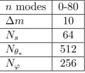
6.2 Tuning parameters . . . 79
6.2.1 Noise . . . 80
6.2.2 Shielding . . . 82
6.2.3 Heating . . . 83
6.2.4 Markers . . . 84
6.3 Transport . . . 84
6.4 Comparison with linear studies . . . 89
6.4.1 Counter-rotation . . . 94
6.5 Comparison with experiment . . . 98
6.5.1 BES system . . . 99
6.5.2 Results . . . 102
6.6 Conclusions . . . 105
Chapter 7 The role of collisions on ITG/TEMs in MAST 106 7.1 Implementation . . . 106
7.2 Linear studies . . . 108
7.3 Nonlinear studies . . . 109
7.3.1 Coarse-graining . . . 110
7.3.2 Number of markers . . . 110
7.4 Results . . . 112
7.4.1 Comparison to experiment . . . 113
7.5 Conclusion . . . 114
Chapter 8 Conclusion 117 8.1 Summary of key results . . . 117
8.2 Future work . . . 119
Acknowledgments
I owe a great deal of thanks to a great many people. First and foremost, I am
grateful to Dr. Erwin Verwichte, my supervisor at University at Warwick, and to
Dr. Samuli Saarelma, my supervisor at CCFE. Both have been instrumental in
helping me produce this thesis, and to survive the trial of completing my PhD.
Erwin stepped in to replace Prof. Arthur Peeters, my original supervisor, who left
in my first year of study for Germany, and his good humour and reassurance has
helped inspire and motivate me through the long, dark teatime of the soul that is
a PhD programme. Samuli’s knowledge and encouragement have helped guide me
and give me a deeper understanding of the physics of tokamaks.
There are many people who, without their knowledge and skills, I would not
have been able to complete this work. Dr. Ben McMillan has provided continuous
help with bendingnemorbto my will and insights into plasma turbulence. Dr.
Al-berto Bottino and Thibaut Vernay have also contributed a great deal of knowledge
and time to my understanding of nemorb. The work done by Dr. Anthony Field
and Young-chul Kim on the BES system, its synthetic diagnostic, and the analysis of
the resulting data, has made this work possible. During my time at Culham, David
Dickinson has proven to be a fountain of useful advice on physics and computers,
and an invaluable sounding board, letting me bounce ideas off him until they
meta-morphosed into crystalline form. Over the last few years, I have benefitted from
useful discussions with a large number of people, including M. Barnes, F. Casson, J.
Cook, D. Edie, S. Freethy, D. Higgins, C. Roach, G. Szepesi, and C. Wrench; there
are certainly others whom I have forgotten.
EP/I501045 and the European Communities under the contract of Association
be-tween euratom and ccfe. The views and opinions expressed herein do not
nec-essarily reflect those of the European Commission. This work was also funded by
epsrcand simulations were performed using thehpc-ffresource at the J ulich
Su-percomputing Centre, thehectornational resource, and theheliossupercomputer
in Japan.
My parents and family deserve a significant proportion of my thanks for their
love and support throughout my education, and for helping me deal with unexpected
crises. Darren Aldous has helped me avoid bad faith through the years, yearn for
eudaemonia, and generally been a friend of mine. I want to thank my friends outside
of physics for their friendship and support, and for putting up with my impromptu
lectures on physics. I have to give special thanks to Nicky for her companionship,
Declarations
I declare that the work presented in this thesis is my own except where stated
otherwise.
This thesis has not been submitted, either wholly or in part, for a degree at
any level at any other academic institution.
Abstract
The free energy in the large temperature and density gradients in tokamaks can drive microinstabilities, which in turn drive turbulence. This turbulence is responsible for the transport of energy and particles over and above that predicted by neoclassical theory. Sheared toroidal rotation can suppress the turbulence and stabilise the underlying microinstabilities, thereby reducing the transport. This thesis investigates how variation of the equilibrium temperature and density profiles, over the same scales associated with the microinstabilities, affects how the flow shear stabilises the linear modes and suppresses the turbulence. A global gyrokinetic code is employed in this investigation, which retains the profile variation and simulates the full 3D domain of a tokamak plasma.
How much flow shear is needed to stabilise the linear ion temperature gradient (ITG) mode is found to be dependent on its poloidal wavenumber, with longer wavelength modes needing more flow shear than the fastest growing mode. This dependence is present whether the flow shear is constant across the radius or if it has the variation typical in an experimental rotation profile. There is an asymmetry with respect to the sign of the flow shear in the effectiveness of the stabilisation, with the maximum linear growth rate occurring at finite negative shearing rates for the plasma studied here. This asymmetry arises from the profile variation, and is found to be significant in simulations of MAST L-mode plasmas, especially when the effects of kinetic trapped electrons are included in the simulations.
Chapter 1
Introduction
1.1
Motivation
We live in a world facing several crises symptomatic of our dependence on limited, environmentally damaging and incredibly useful fossil fuels - increasing geopolitical
tension, global climate change, and irresponsible waste of resources[2]. Development
of methods of energy production which do not rely on limited or easily monopolised resources has become a clear and pressing global goal[3]. Currently, the largest
focus from both the public and private sectors worldwide is on socalled renewables
-wind, solar, tidal, etc[4]. These work well on local scales, but suffer from severe lim-itations on national and international scales. The other major fossil fuel-alternative
is nuclear fission. This method suffers from an almost crippling perception of
be-ing excessively dangerous with an unsolvable waste problem, as well as havbe-ing its own legitimate concerns - proliferation of nuclear materials is an not-inconsiderable
problem.
Fusion promises unlimited, clean and safe energy. Research has been
under-way since the 1950s, but the early optimism was tempered as experiments failed
to live up to the dream. Some of that optimism is now returning, as we come to understand more and more of the physics of fusion plasmas and achieve more and
more goals of the fusion experiment. We can produce fusion reactions - the next
step is achieve self-sustaining reactions. This is hoped to be achieved using the internationally developed ITER, which is scheduled to have its first plasma in 2020.
After ITER, a prototype power plant will be built, named DEMO. DEMO is hoped
Figure 1.1: Binding energy per nucleon versus number of nucleons for all known nuclides. There is a peak in the binding energy at 56Fe. Elements beyond this cannot be created through the usual stellar fusion reactions, and must be formed in the violent explosions of stars. Data for this figure was taken from [5]
1.1.1 What is fusion
Fusion happens when two nuclei come close enough that the strong force becomes
dominant over the repulsive Coulomb force, binding them together. The resulting product has a smaller mass than the original nuclei as some of the mass is in the
strong force holding the nucleons together, the binding energy, and the binding
energy per nucleon is less in the product than in the reactants. The “missing mass” is released as energy. The binding energy is the energy required to separate a nucleus
into its component nucleons. Figure 1.1 shows the binding energy per nucleon of all known nuclides, and it can immediately be seen that there is a peak in this graph.
This means that fusion reactions up to 56Fe are exothermic, and as such, all these
elements can be produced in stars. Elements heavier than 56Fe can only be created in supernovae and in laboratories on Earth. The most energetic fusion reactions are
those that produce helium from isotopes of hydrogen.
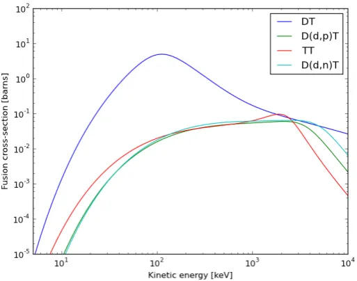
The probability of a given fusion reaction occurring is measured by its cross-section. As mentioned above, reactions producing isotopes of helium release the
most energy, and of these, deuterium-tritium → helium-41 (hereafter referred to
as D-T) has the largest cross-section (see fig. 1.2). For these reasons, D-T is the
Figure 1.2: Fusion cross-sections for some common reactions as functions of energy: blue, DT; red, TT; green and turquoise, DD. Note the resonance of the DT reaction around 100 keV.
reaction most favoured by most fusion power plant designs.
Triple product
In a fusion power plant, it is essential that we can get more energy out than we
put in. The power lost (PL) through inefficiencies in the power generation, loss
mechanisms internal to the plasma, etc., must be less than that put into the plasma
through external heating (PH) and self-heating by alpha particles (Pα). If the
alpha-heating is equal to the power loss, then the plasma is said to have achieved ignition. The ignition condition is set by three parameters: the plasma temperature, density
and energy confinement time,τE = PWL, whereW is the energy stored in the plasma.
For a typical D-T reaction, the ignition condition is[6]:
nT τE >1021m−3keV s, (1.1)
also known as the “triple product”. In tokamaks, the density has an upper limit
(that depends on the plasma current), set by the Greenwald stability criterion[7], and the temperature has a small optimum range (see fig. 1.2), leaving only τE as
a free parameter2. The optimum range of temperature has a lower limit set by
2
This only applies to tokamaks. In ICF, there are different limits tonandT, though the triple
the peak in the cross-section and an upper-limit set by the operating regime of the
device. Increasing the temperatures means increasing the plasma pressure, which means magnetic field required to contain the plasma must also be increased (this
is discussed in more detail in section 1.2.2). The energy confinement time is set by
the transport of heat from the core of the plasma to the outside (see section 1.3 for more about transport).
1.2
Magnetic confinement
In order to have a sustainable reaction, it is necessary to hold the plasma together
in one place long enough to confine the energy. There are three main methods of
confining plasmas for fusion reactions - gravitational, inertial and magnetic. Grav-itational confinement is used by stars. The huge mass of plasma contracts under
its own gravity, increasing the temperature and pressure to levels where fusion is
possible. The star needs enough mass to counteract the radiation pressure exerted by the energy released in its fusion reactions. The engine of stars is the p-p reaction,
but because it is mediated by the weak interaction and has a small cross-section,
this reaction is slow.
Inertial confinement uses lasers to heat a small pellet, ablating the outer
layers. The resulting explosion causes the core to implode, creating high densities
and pressures. This is one of the current leading efforts to achieve fusion power, with several state-of-the-art projects underway, namely NIF and HiPER.
Magnetic confinement is the other contender for fusion power. Because
plas-mas consist of electrically-charged particles, it is possible to confine them within magnetic fields. Charged particles in a magnetic field experience a force
perpendic-ular to both the magnetic field and their velocity. This means that the particles
gyrate in closed-orbits in the plane perpendicular to the magnetic field, given uni-form, homogeneous fields. This motion is called the Larmor motion, and has a
characteristic radiusρL (also called the Larmor radius, cyclotron or gyroradius):
ρL=
mv
qB, (1.2)
wherem, v, q are the mass, velocity and electric charge respectively of the particle, and B is the magnetic field strength. The particle gyrates with a frequency Ωc =
qB/m, (called the cyclotron frequency). Parallel to the magnetic field, particles can
turns out that this by itself is not sufficient. It is necessary to also include a degree
of helicity in the field lines in order to prevent system-scale instabilities[8]. For example, the∇B drift causes the electrons and ions to move vertically in different
directions, causing a separation of charge, leading to a massive loss of particles due
to theE×B drift (see section 1.2.1 for an explanation of these drifts). There are two ways to achieve this helical field: either by using magnetic coils especially shaped
to directly produce this field, or by driving part of the fields through a current in
the plasma. The class of machines using the former approach are called stellarators, while the latter are called tokamaks (the Russian acronym of “toroidal chamber with
magnetic coils”). The plasma current is usually driven by changing the electrical
current through the central solenoid (so-called ohmic operation), meaning most tokamaks are inherently pulsed 3. This is contrast to stellarators, whose design
means they can be run almost indefinitely. However, the geometry of the stellarator
field coils is exceedingly complicated, making them costly to design and build. The induced plasma current has a secondary benefit, in that it also heats the plasma.
So far, the highest values of the triple product in magnetic devices have been in
tokamaks.
1.2.1 Single particle motion
Charged particles in a magnetic field gyrate around the field lines with a
character-istic radius,ρLand can be accelerated along the field either by parallel electric fields
(Ek) or the magnetic field strength decreasing along the field line (∇kB). Forces
perpendicular to the magnetic field applied to the particles induce a drift which is
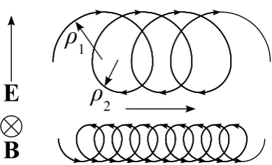
perpendicular both to the field and to the external force. There is a simple phys-ical picture to understand this motion, as illustrated in fig. 1.3. When the force is
parallel to the particle’s instantaneous velocity,ρL is temporarily increased. When
it is anti-parallel to the velocity, ρL is decreased. This combination causes a drift
perpendicular to the applied force,Fof the general form:
vD =
F×b
qB , (1.3)
whereb=B/Band B is the magnitude of the magnetic field.
The main drifts in a tokamak are due to the electric field and the curvature
and (perpendicular) gradient of the magnetic field. The force due to the electric field depends on the charge of the particle - it is immediately clear that the resulting drift
3
Figure 1.3: Charged particles in the presence of both a magnetic field and an electric field gyrate around a guiding centre which experiences a drift perpendicular to the two fields. This cartoon demonstrates how this drift arises. On one side of its orbiting, the particle has an increased gyroradius, ρ1, while on its other side, it
is decreased, ρ2. The top spiral shows the motion of a positively charged ion, the bottom, an electron. Though the two species gyrate in opposite directions, the electric field accelerates them in opposite directions - the resulting E×B drift is independent of charge. The other drifts discussed in this section, however, do depend on charge, and so ions and electrons drift in opposite directions.
is independent of charge:
vE×B=
E×b
B . (1.4)
It can be seen that the perpendicular E×B drift is also independent of mass
-ions and electrons feel the same drift in the same direction. Electric fields do not immediately lead to a charge separation, as might na¨ıvely be expected.
On the other hand, curvature of the magnetic field and perpendicular gradi-ents in the field do lead to separation of charges. The curvature drift comes about
because particles following curved field lines experience a centrifugal force outwards,
while the∇B drift arises because the magnetic moment (µ=mv2⊥/2B) of the par-ticle is an adiabatically conserved quantity. That is, provided that the changes in
the magnetic field are slow compared to the gyrofrequency and larger than the
gyro-radius, the flux enclosed by the particle’s orbit is almost constant. These two drifts have similar forms and are often combined into one expression:
vd=
mvk2+12mv⊥2
ZeB
b× ∇B
B , (1.5)
A time-varying electric field can also lead to a charge separation, which itself leads to the so-called polarisation drift. This has a slightly-different form to the
previous drifts:
vp =
m
eB2
dE
We can then decompose the motion of a particle into the gyro-motion about
a guiding centre, its parallel motion along the field line and the perpendicular drifts. If we ignore the gyro-motion and instead concentrate on the motion of the guiding
centre,X, we get
vX=vkb+vd+vE×B+vp. (1.7)
The origins and mechanisms of heat and particle transport are discussed
in-depth in section 1.3.
1.2.2 Tokamak equilibria
The helical field in tokamaks has two components: the toroidal field (Bϕ), produced
by the toroidal field coils; and the poloidal field (Bθ), produced by the plasma
current and poloidal field coils. The shape of the helical magnetic field is such that the field lines lie in toroidal surfaces and are axisymmetric to within a few percent.
We can define a convenient radial coordinate,ψ, as the poloidal magnetic flux within
a magnetic surface. It can be shown thatψ is constant on a magnetic surface, i.e. that
B· ∇ψ= 0, (1.8)
so these surfaces are often called flux surfaces. From eq. (1.8), we get the following
relations between the poloidal field andψ:
BR=−
1
R ∂ψ
∂Z, BZ =
1
R ∂ψ
∂R, (1.9)
which along with Gauss’ Law which requires:
1
R ∂
∂R(RBR) +
∂BZ
∂Z = 0, (1.10)
whereZ is the vertical direction in fig. 1.4.
Our most basic coordinate system for a tokamak is then (ψ, θ, ϕ) (see fig. 1.4).
For convenience, we will often refer to “parallel” and “perpendicular” directions -these are understood to be relative to the magnetic field, B, and lie within a flux
surface (that is, the perpendicular direction is∇ψ×∇ϕ). Note that “perpendicular” may also refer to the perpendicular plane - i.e. a poloidal cross-section of the plasma
at constantϕ.
In equilibrium, the pressure and Lorentz forces are in balance:
Figure 1.4: Illustration of the shape of two tokamak plasmas - the outer torus shows a large aspect-ratio plasma, with circular cross-section; the inner torus depicts a small aspect-ratio plasma. Also shown is the general coordinate system of a tokamak: the “long way round” the torus is the toroidal direction,ϕ; the “short way round” is the poloidal dimension,θ. The vertical dashed line is the axis of symmetry. The minor radius,r, and major radius, R, as well as the flux surface label,ψ are indicated. A representation of the shape of the magnetic field,B, is shown winding around a flux surface.
whereJis the plasma current density and pis the pressure. From this equation, it is immediately obvious both thatB· ∇p= 0 and thatJ· ∇p= 0, and so bothJand
Blie on surfaces of constant pressure. This is made transparent when we introduce a current flux function,f, related to the poloidal current density by
jR=−
1
R ∂f
∂Z, jZ =
1
R ∂f
∂R. (1.12)
Using Amp`ere’s equation, we can then show that
f = RBϕ
µ0
. (1.13)
Given eq. (1.12) and eq. (1.11), it follows that
∇f × ∇p= 0, (1.14)
and so, knowing thatpis a function ofψ, it must be true thatf =f(ψ). Therefore,
B and J are both flux functions, and we need only to use ψ as our flux function.
The safety factor,q, is used to measure the degree of helicity of the magnetic
field. More precisely, it is defined as:
q = 1
2π
Z 2π
0
B· ∇ϕ B· ∇θ0dθ
0
. (1.15)
The safety factor is so-called because its profile determines some of the major
sta-bilising properties of a tokamak equilibrium. Large, system-scale
magnetohydrody-namic (MHD) instabilities become serious disruptive events whenq drops below 3 at the edge, for example[9].
An important quantity in tokamaks is its plasma-β, the ratio of plasma thermal pressure,p=nT to its magnetic pressure:
β= p
B2/2µ
0
. (1.16)
This is a dimensionless ratio which measures the efficiency of confinement due to the
magnetic field. In tokamaks,β must necessarily be smaller than 1, as β >1 means
that the magnetic pressure is too small to balance the thermal pressure. Typically, it is only a few percent, though in spherical tokamaks, it may reach as much as 30%.
1.2.3 Magnetic mirroring and trapped particles
As mentioned above, particles moving into regions with increasing magnetic field strength experience a force parallel to the motion of their guiding centre. This is a
consequence of the conservation of both the total kinetic energy, 12m(v2k+v⊥2), and the magnetic moment,µ. The magnetic moment is not strictly a constant of motion - rather, it is an adiabatic invariant, and remains constant provided the magnetic
field changes slowly enough. That is, the spatial variation in the magnetic field
should be larger than the Larmor orbit, and the temporal variations longer than the gyro-period. Provided these conditions are met, the magnetic moment will be
conserved. The increase in B must be matched by an increase in v⊥2 to keep the flux enclosed by the particle’s gyration constant. Then, to balance this, vk must
correspondingly decrease. At some point in the particle’s trajectory, the parallel
velocity may become zero, and this “mirror force” will start to move the particle back the way it came. In order to overcome the mirror force, particles must have
some minimum vk - these are called “passing” particles. Those who do not are
termed “trapped” particles. In a tokamak, the toroidal magnetic field varies with major radius, roughly as ∼ 1/R. As a particle follows a field line, it will see a
that particles can be trapped on the outboard side (also called the high field side),
bouncing between two points along a field line, if their vk is not large enough The
minimumvk can be shown to be given by:
vk >
r
2
1−v⊥, (1.17)
where=r/R0 is the inverse aspect-ratio at the particle’s position, and R0 is the major radius of the magnetic axis (where Bθ → 0). In addition to this trapped
motion, particles also experience a deviation from the flux surfaces due to
conser-vation of the canonical momentum, pϕ =mRvϕ+qψ. It is obvious that changing
vk must lead to a change in ψ. The size of the excursion from the flux surface can
be calculated, and the width of a banana orbit,wb can be shown to be:
wb =
q
√
ρL. (1.18)
Importantly, two particles of the same species with different signs ofvk drift to
dif-ferent sides of a flux surface. Several significant effects arise because of this. Firstly,
at a given radius and assuming a density gradient, there will be more particles with
one sign of vk than the other. This leads to a the so-called diamagnetic drift, as
there are more particles moving in one direction. The sign of this drift is different
for ions and electrons. The second effect of the banana orbits is the bootstrap
cur-rent. The trapped particles carry some parallel current due to their motion along the field lines. Friction between the trapped and passing particles then leads to
another, larger current carried by the passing particles, which is known as the
boot-strap current. Bootboot-strap currents are important because it is possible to use them to replace some or all of the induced plasma current to maintain the poloidal field,
and as such, could be used in future steady-state devices.
1.3
Transport in tokamaks
Why don’t tokamaks work? Early research suggested that a working reactor could
be built by 1970[8]. The reason for this overly-optimistic prediction was the under-estimation of transport. The transport of heat, energy and particles determine the
confinement times of the respective properties and early theories were based around
collisions mediating the transport (“neo-classical theory” - see section 1.3.1). The observed transport turned out to be an order or magnitude larger than predicted
achieve-Figure 1.5: Particles can become trapped on the low-field side by magnetic mirror effects. The shape of their orbits, projected onto the poloidal plane, have a char-acteristic banana shape (the gyro-motion of the particles is not shown here). In this example, following the particle from its lowest point, it experiences a vertical drift downwards which pulls it off the flux surface (dotted line). As it travels anti-clockwise, it crosses the outboard mid-plane, at which point, the vertical drift pulls it back to the flux surface. As it reaches the top of its orbit, itsvk reverses and the
vertical drift now pulls it below the flux surface.
ment of ignition. We now know that turbulence is responsible for the anomalous
transport, and the study and control of turbulence has preoccupied not only the fusion community, but indeed modern physics, and it remains one of the great open
problems of science.
1.3.1 Classical and neoclassical theory
The most basic transport mechanism is a purely collisional diffusive process. We can
calculate the magnitude of the diffusion coefficient,D, of this process from a simple
random walk model. We get thatD∼(∆x)2/∆t, where ∆xis the step size and ∆t
is the time scale of the collisions. In a tokamak, the step length is the gyroradius,
so:
D∼ρ2Lν, (1.19)
whereν is the collision frequency. If confinement were limited solely by this simple
diffusion, then the confinement time would be
τ ∼ a
2
D =
a
ρL
2
1
ν. (1.20)
It is important to note here that collisions between two particles of the same species
will produce no net transport of particles. It is collisions between ions and electrons
[image:22.595.254.391.107.230.2]radius of the electrons, ρe, and the collision frequency is that of electron-ion
colli-sions, νei 4. However, diffusion of heat is different - collisions between like species
can exchange energy, and so can transport heat. Therefore, the heat diffusivity of
ions, χi, is greater than that of electrons, χe, by factor of the square root of the
mass ratio:
χi ∼
r
mi
me
χe. (1.21)
Given a typical electron-ion collision rate of 0.1−1kHz, and ρe ∼1 mm, a∼1 m,
the confinement time from this simple diffusion process would be on the order of an hour. This shows the source of the optimism in early fusion experiments - a device
only a metre across could be sufficient to meet the energy demands of an entire city. The collisional process outlined above changes dramatically when we include
the magnetic geometry of a tokamak. Diffusion coefficients can increase by several
orders of magnitude. We call the collisional theory that includes effects derived from tokamak geometry “neoclassical” to differentiate it from the picture above, which
is called “classical”. The first big effect arises from trapped particles undergoing
banana orbits (see fig. 1.5). The step size of the diffusive process then becomes the width of this banana orbit, rather than the gyroradius. However, because only
a fraction, ∼ √, of particles are actually trapped and in banana orbits, so the
effective diffusivity is actually
Def fban∼ q
2
3/2ρ
2
eνei. (1.22)
Again, the electron and ion particle diffusion rates cannot be different, whereas the heat diffusivities differ between species by a factorqmi
me. This process is only
impor-tant at low collisionality, where particles complete at least one orbit before they are
scattered. At higher collisionalities, where the collisional frequency becomes com-parable to the bounce frequency, different mechanisms dominate the diffusion. Two
regimes exist for higher collisionalities - the plateau regime, where the diffusivity no
longer depends on collisionality, and the Pfirsch-Schl¨uter regime, which has a weaker dependence onν than the banana regime[9]. However, due to the high temperatures
in tokamaks, they have rather low collisionalities and so only the banana regime is of interest5.
4
In this thesis, we will denote quantities peculiar to electrons or ions with a subscript e or i,
respectively. Ions are assumed to be deuterium ions, unless otherwise stated
5
1.3.2 Anomalous transport and turbulence
The strong gradients in temperature and density in tokamaks provide large amounts
of free energy. As a result, there is a whole zoo of instabilities that can tap this
energy and drive increased transport of heat and particles. Large, system-scale in-stabilities tend to affect the stability of the plasma equilibrium itself, therefore, for
stable equilibria, it is the smaller scale so-called “microinstabilities” that are the
most important to consider. Chapter 3 shows the main class of microinstabilities, drift waves, are linearly driven. When they reach a certain amplitude, the
microin-stabilities can start to nonlinearly interact and the plasma becomes turbulent. In
experiment, the linear growth phase is never seen - we only see turbulent fluctuations in density, temperature, magnetic field, etc. Fluctuations in density,δn, cause
fluc-tuations in the electrostatic potential,δφ, which in turn produces anE×B velocity (this is discussed in more depth in chapter 3):
δv⊥=
δE⊥
B . (1.23)
From this fluctuating velocity, and the original density fluctuation, a convective flux
arises:
Γ =hδv⊥δni, (1.24)
where the angular brackets signify an average over a flux surface. How these fluctu-ations arise and interact will be discussed in more detail in chapter 3. Fluxes for the
ions from fluctuations turned out to be an order of magnitude or more larger than
neoclassical predictions[9]. More than this, heat fluxes for the electrons were the same level as those for the ions - in direct contradiction to before. We can glean the
reason for this from a mixing length argument, which is simply that the
microin-stabilities stop growing when their linear growth rate,γ, is balanced by the rate at which they are dissipated. This turns out to be the turbulent diffusion rate, which
for a perpendicular wavenumber k⊥ is given by : γD ∼k2⊥D[10]. Rearranging, we
get the quasilinear turbulent diffusion coefficient:
D∼ γ
k⊥2 . (1.25)
Electron-scale microinstabilities, despite having a much shorter wavelength, have
1.4
The MAST device
1.4.1 Spherical tokamaks
Spherical tokamaks (STs) are a class of device with a small aspect-ratio,R0/a∼1,
whereais the minor radius of the largest flux surface (cf. the typical aspect-ratio of a conventional tokamak of∼2.5). They are often likened to a “cored-apple” rather
than the “doughnut” or “bagel” of larger aspect-ratio machines (see fig. 1.4 for an illustration of the difference). The small aspect-ratio means that STs can have a high
fraction of trapped particles. This makes them susceptible to microinstabilities that
are driven by trapped particles, but it also means they can have larger bootstrap currents (toroidal currents driven by particles in banana orbits). Their low moment
of inertia means that STs can be easily spun up to high rotation rates by injected
neutral beams. This makes them an ideal place to study the effects of strong flows. Because of their size, STs have a smaller potential as power sources, as fusion
power scales with volume[11]. However, their size does mean that the neutron fluxes
will be much higher. There are plans to use STs as “component test facilities”, where materials can be subject to large neutron fluxes, simulating conditions in
larger machines.
The main advantage of spherical tokamaks is that, due to their size and shape, it is possible to achieve higher a plasma-β than conventional aspect ratio
tokamaks[11]. This means that they can use a smaller toroidal field to confine a
given kinetic pressure. As one of the biggest costs of running a tokamak is the production of the magnetic field, this means that STs would be cheaper to build
and run for the same fusion power.
1.4.2 Local vs. global analysis
Over the years, there have been many different models and frameworks used to
ad-vance our understanding of plasmas. One of the first attempts was the MHD, single
conducting fluid model. As will be covered in chapter 3, the correct, separate treat-ment of electron and ion dynamics is necessary to understand microinstabilities[12].
It is possible to use two fluid models to recover many of the qualitative features
of microinstabilities. However, the features of turbulence and microinstabilities themselves suggest a different approach: gyrokinetics. Chapter 2 will describe the
gyrokinetic formalism and derive the relevant equations. We restrict ourselves to
the collisionless and electrostatic limit. For details of collisional terms see [13] and for electromagnetic terms, see [14].
gyrokinetic approach utilises. A common assumption is that the normalised
gyro-radius,ρ∗=ρi/a, becomes vanishingly small. In this limit, usually called the “local”
limit, it can be assumed that flux surfaces are independent of each other. Numerical
codes which use this limit (hereafter referred to as local codes) make the assumption
that equilibrium quantities and their derivatives are constant across the simulation domain, e.g. T0 and dT0/dψ both take a single, constant value at all points in the
simulation. This approach is valid in the limit ρ∗ → 0 as the simulation is only
looking at an infinitesimally thin slice of the whole system. In large aspect-ratio devices, such as JET or ITER, this limit is a good assumption. We can check this
by looking at quantities which vary withρ∗, such as the growth rate of a particular
instability. Figure 1.6 shows that ρ∗ = 1/500 means that the local approximation
0 50 100 150 200
0 0.05 0.1 0.15 0.2
1/
ρ
*γ
[v
th
/a]
global NEMORB local GS2
Figure 1.6: Variation of the growth rate of the ITG mode withρ∗, the normalised
gyro-radius. The value ofρ∗ on the MAST device are indicated. Figure taken from
[15]
is a good assumption for JET plasmas. Local codes may have simulation domains of the order 100ρi in the “radial” direction6. However, MAST can haveρ∗ ∼1/50,
and so these local codes may have radial domains larger than the MAST machine.
This large ρ∗ means that it is necessary to use a numerical code which captures
the full radial variation of equilibrium quantities. Codes which keep variation of
the equilibrium profiles are called “global codes”. We will show in chapter 5 that
retaining profile variation can have significant effects on the predictive abilities of numerical codes.
Another important feature of MAST is that it has a small aspect-ratio and
6
highly shaped flux surfaces. This means that in addition to profile effects, geometry
effects are also important - it is not possible to make the “large aspect-ratio” (R/a
1) assumption, where
q = rBϕ
R0Bθ
. (1.26)
This assumption turns out to be convenient for reducing the complexity of many equations in tokamaks, such as the formulae for the magnetic equilibria. Because
MAST has a small aspect-ratio, the full expression forqmust be used (see eq. (1.15)),
and the magnetic equilibrium quantities are often two dimensional functions of (ψ, θ). Geometry effects are not limited to global codes, and many local codes do
include them. Simple models for the magnetic equilibrium, such as s-α or circular
cross-sections, are ruled out though.
The numerical code, nemorb, used in this thesis to study MAST plasmas
has all of these effects. It is a global code, solving the full 3D domain, with realistic
geometry taken from experimental data. The physical model used is gyrokinetics, where the rapid gyro-motion of particles is averaged over, reducing the problem
by one dimension. Gyrokinetics is discussed in more detail in chapter 2. During
the undertaking of the work in this thesis, the code was in a state of development, and had only electrostatic fluctuations. In general, due to their relatively high
β, electromagnetic effects are important in STs. However, simulations using the
local gyrokinetic codegs2show that while for H-mode discharges, electromagnetic effects are indeed crucial, they are not as important for L-mode shots[16], such as
the one studied in this thesis. Electromagnetic effects have recently been included
innemorb[14], and further work will incorporate these.
1.5
Outline
This introduction has given a sketch of some of the important physics in tokamaks. The rest of this thesis presents a more in-depth study of a few of the more important
pieces necessary to understand the work presented herein. The reader’s attention is
directed to [8, 9, 17, 18] for more detail on tokamak equilibria and possible magnetic geometries, and to [19, 20, 21] for a more complete understanding of transport in
tokamaks. The MAST physics reports, [22, 23], outline many of the past and current
physics problems and studies of the MAST device.
The main body of work of this thesis is presented in chapters 5 to 7. Chapter 5
introduces background toroidal rotation to linear simulations of MAST plasmas
the machine. The next two chapters focus on nonlinear simulations. At first, in
chapter 6, we include only the background rotation, and explore its effect on heat and momentum transport. Then, in chapter 8, a synthetic diagnostic is used to
compare the simulations to real experimental data. Additional physics, in the form
of collisions, are also included.
Chapter 2 derives the model used innemorb, while chapter 4 discusses the
coordinate system, equations used and assumptions made in the code. The physics
Chapter 2
Gyrokinetics
2.1
Introduction
The magnetic field in tokamaks separates the plasma into two distinct regions, sepa-rated by the “separatrix”. The Last Closed Flux surface (LCFS) defines the
bound-ary, although in reality, this is not a sharp transition. Outside of the separatrix
field lines are “open”, ending on the divertor of the tokamak1. The plasma in this region is characterised by low densities and temperatures which also can have
vari-ation along the field lines, as well as large fluctuvari-ations[24]. By contrast, inside the
separatrix (the “core”), field lines are closed and the plasma here has much higher densities and temperatures (which remain flux functions), and comparatively small
fluctuations[24]. They are non-relativistic (vth c), classical (degeneracy
condi-tion), fully ionised and fulfil the quasi-neutrality condition[9]. While the edge of a tokamak plasma (the region close to the LCFS) contains a great deal of interesting
physics, and sets the boundary conditions for the core, this thesis deals exclusively with the core.
The large number of particles in a tokamak plasma all generate their own
electromagnetic fields, which interact with every single other particle in the plasma. This clearly necessitates a statistical description for the evolution of the plasma.
The particles are distributed in a six dimensional phase space, according to the
dis-tribution functionfs(x,v, t) for speciess, with spatial coordinatesx,and velocities
v. The mass continuity equation tells us that the mass flow out of a closed volume
is equal to the rate of change of mass density in that volume. By analogy, we can
construct a similar continuity equation for the distribution function - Liouville’s theorem states that the flow out of a closed volume of phase space is equal to the
1
rate of change of the probability density:
∂fs
∂t +
dx
dt · ∇fs+
dv
dt ·
∂fs
∂v = 0, (2.1)
where we have assumed that there are no sources or sinks of particles, and that there are no collisions. The coupling between species is therefore mediated solely by
the electromagnetic fields. This is known as the Vlasov equation[9] and by itself is
not enough to fully describe the complex behaviour of plasmas. Maxwell’s equations provide the rest of the physics needed to describe all the phenomena present in the
core of tokamak plasmas.
Unfortunately, the Vlasov-Maxwell system of partial differential equations is not tractable analytically for most plasmas of interest, and is not even numerically
tractable for real world plasmas. In order to have a chance at solving these equations,
we must make assumptions and simplify the system.
Over the years, there have been many different models and frameworks used
to advance our understanding of plasmas. One of the first models was the MHD,
single conducting fluid2. This model has been employed to great success over the years, and is still used for many plasma calculations, especially those involving the
equilibrium structure and major instabilities. However, there are some plasma
phe-nomena that this model is unable to deal with. As will be covered in chapter 3, the correct, separate treatment of electron and ion dynamics is necessary to understand
microinstabilities. It is possible to use two fluid models to recover many of the qualitative features of microinstabilities. However, the features of turbulence and
microinstabilities themselves suggest a different approach: gyrokinetics. This
chap-ter will describe the gyrokinetic formalism and derive the relevant equations. We restrict ourselves here to the collisionless and electrostatic limit as this is the regime
in which all the work in this thesis has been performed. For details of collisional
terms see [13] and for electromagnetic terms, see [14].
2.2
Gyrokinetic ordering
Gyrokinetics is motivated by the large range of temporal and spatial scales found
in fusion reactors. Time scales vary from the cyclotron frequency (Ωci ∼ 108 Hz,
Ωce ∼ 1011 Hz) up to shot times (100 s), eventually up to steady-state reactors
(months +). Spatial scales vary from the Larmor radius (ρi ∼1 mmρe∼0.01 mm)
up to the system size (L ∼ 1 m). This large variation in scales is a challenge for
2
theory and simulations. Fortunately, most of the scales are well separated, and we
can use this to our advantage. The gyrofrequency is much faster than almost all of the physics of interest - for example, the typical turbulence frequency is of the order
100 kHz[25]3. Knowing this (and the orderings given below), we can average over
the fast gyromotion of the particles. This is the heart of gyrokinetics. Removing the rapid gyrations of particles is equivalent to reducing the dimensionality of the
system and we move from a phase space with six dimensions (three of space, three
of velocity), to one with five - losing a dimension of velocity.
More formally, we can define a small parameter, ω, that reflects that the
frequency of the fluctuating quantities, ω we are interested in is much slower than
the cyclotron frequency:
ω
Ωc
∼ω 1. (2.2)
It is also possible to separate spatial scales, as long as the gradient of the magnetic field is much longer than the Larmor radius. We can define another small
parameter:
ρi
LB
∼B 1, (2.3)
whereLB is the logarithmic gradient length scale of the magnetic field
1
LB
=|∇lnB|=
∇B B
. (2.4)
We also require that the length scales of the background equilibrium quantities, such as the temperature,T, and density,n, are of the same order
ρi
Ln
∼ ρi
LT
∼B. (2.5)
The amplitude of fluctuations in the bulk density,δn,and electrostatic
poten-tial,δφin tokamaks is typically much smaller than the magnitude of the equilibrium
quantities. This represents a third small parameter:
δn
n ∼
eδφ
T ∼δ 1. (2.6)
Note that throughout this thesis, the temperature is given in units of energy, i.e.
T =kBTK, whereTK is the temperature in Kelvin and kB is the Boltzmann
con-stant. Given these three small parameters, we can expand all the relevant equations in them, keeping only the terms up to a certain order. This reduces the
computa-3
tional effort required to simulate a plasma, while ensuring that errors are still small
compared to the physics.
In general, the different small parameters are assumed to be the same order:
ω∼B ∼δ, (2.7)
however, one of the advantages of the gyrokinetic ordering is that this can be altered if need be. Additional orderings may also be introduced, without destroying the
structure already in place.
2.3
Lie formalism
The Lie formalism ensures that the conservation laws are preserved throughout the
transformation from real space to gyro-space. This guarantees a solid mathematical foundation for the whole system, and maintains energy and momentum
conserva-tion even to the lowest order in the expansion. The Lie-Transform method involves
two changes of coordinates: the first, from the real space coordinates of the particle (x,v) to the guiding centre coordinates (X, vk, µ, α); then from the guiding centre
frame to the gyro-centre frame ( ¯X, vk,µ,¯ α¯). Figure 2.1 illustrates the particle and
guiding centre frames. The difference between the guiding centre and gyro-centre frames is the inclusion of the perturbed fields in the latter. Because the length
scales of the perturbed fields can be the same size as the gyroradius, they modify
the gyromotion, destroying the conservation of µ. The Lie-Transform method is based around the Hamiltonian formulation, using a series of “near-identity”
trans-formations and the freedom of gauge invariance to remove the rapid gyromotion and
define a new quantity (¯µ=µ0+µ1+. . .) which is conserved. These transformations are formally an asymptotic expansion in powers of the small parameterδ, defined
in eq. (2.6), and can be formulated out to any arbitrary order, with the zeroth order (the guiding centre transformation) being expressed in terms of B. It is usually
sufficient to derive them only to second order4.
The derivation of the equations proceeds as follows:
i) formulate the Lagrangian in particle space,x(section 2.3.1),
ii) transform the Lagrangian to guiding centre space, X (section 2.3.2),
4
B
x
X
(a)
B
(b)
Figure 2.1: Schematic of the gyrokinetic framework. a) A charged particle gyrates around a field line, B, and drifts cause the guiding centre motion (dashed line) to move off the field line. The particle’s position vector is indicated by x, while the position vector of the guiding centre isX. b) The difference between the guiding-and gyro-centre coordinates is the inclusion of the perturbed fields in the gyro-centre frame.
iii) use a Lie transform to move to gyro-centre space, ¯X(section 2.3.3),
iv) derive the gyro-form of the Poisson equation (section 2.5).
2.3.1 Lagrangian in particle space
We first formulate the Lagrangian in the particle space,x. We use Einstein notation,
where pairs of repeated indices imply a summation over those indices. Latin indices
are over spatial coordinates, and Greek indices over spatiotemporal coordinates, i.e.
i, j∈ {1,2,3}
µ, ν ∈ {1,2,3,4} (2.8)
The Lagrange equations of motion (for a single particle) are:
d dt
∂L
∂q˙i
− ∂L
∂qi
= 0, (2.9)
where (q,p) are canonical variables and the Lagrangian is
L=p·q˙ −Hc(q,p, t). (2.10)
We can then generalise this to an arbitrary phase space,z=z(q,p, t):
The Poincar´e-Cartan fundamental one-form is
γ ≡ Ldt=γidzi−Hdt≡γµdzµ (2.12)
Then for a given coordinate transformation: Zµ=Zµ(z, t)
γ =γµdzµ= ΓµdZµ, (2.13)
where
Γµ=γν
∂zν
∂Zµ (2.14)
We can then form the Euler-Lagrange equations:
ˆ
ωij
dzj
dt = ∂H
∂zi
+∂γi
∂t, (2.15)
where
ˆ
ωij =
∂γj
∂zi
− ∂γi
∂zj (2.16)
are the components of the 8×8 antisymmetric Lagrangian tensor, also called the symplectic structure5.
The Euler-Lagrange equations are invariant under gauge transformation:
γ =γ+ dS ∀S(z) (2.17)
The canonical Hamiltonian for a single charged particle in a magnetic field
with a perturbed electrostatic field,φ, is
H(q,p, t) = 1
2m
p−eA(q)2+eφ(q, t), (2.18)
whereA is the vector magnetic potential.
We now specify our coordinates as:
x=q
v= m1(p−eA). (2.19)
5
This essentially means that volumes in 6D phase space are conserved under a given
Our one-form is now:
γ =γidzi−Hdt
=eA(x) +mv]·dx−12mv2dt−eφ(x, t)dt (2.20)
=γ0+δγ, (2.21)
where
γ0 =
eA(x) +mv]·dx−1
2mv
2dt, δγ =−eφ(x, t)dt (2.22)
are the zeroth order and perturbed one-forms respectively.
2.3.2 Guiding centre transformation
Transformation into the guiding centre-frame is done using the following
relation-ships to real space:
x=X+ρ(X, α), (2.23)
vk =v·b(x), (2.24)
µ= mv
2
⊥
2B(x), (2.25)
α= tan−1
v·ˆe1 v·ˆe2
, (2.26)
where
ρ(X, α) =ρ(x)g, (2.27)
g= [ˆe1cosα−ˆe2sinα], (2.28)
and ρ is the gyroradius vector pointing from the guiding centre to the particle’s position, ˆe1,2 are arbitrary orthogonal unit vectors in the plane perpendicular to b=B/B, the magnetic field unit vector.
Using the above relations, expanding the vector potential aboutx'X, and dropping terms beyond first order, we get:
A(x) =A(X) + v⊥
Ωg· ∇A, (2.29)
dx= dX+ 1
Ωgdv⊥+
v⊥
Ωhdα, (2.30)
of eq. (2.20) using eqs. (2.29) and (2.30), we get the guiding centre one-form:
Γ0 =
n
eA(X) +ev⊥
Ω (g· ∇A) +mv
o
·dX
+
ne
ΩA(X)·g+
ev⊥
Ω2 (g· ∇A)·g+ m
Ω(v·g)
o
dv⊥
+
nev⊥
Ω A(X)·h+
ev⊥2
Ω2 (g· ∇A)·h+
mv⊥
Ω (v·h
o
dα
−(12mvk2+µB)dt. (2.31)
This form of the Lagrangian still contains dependencies onα(terms containingg,h).
We are free to choose the gauge thanks to eq. (2.17), so we choose
S=−ev⊥
Ω g·A−
1 2
ev⊥2
Ω2 (g· ∇A)·g, (2.32)
⇒dS=−e
Ω
h
(g·A)dv⊥+v⊥(A·h)dα+v⊥(g· ∇A)·dX i
−ev⊥
Ω2 (g· ∇A)·gdv⊥− 1 2
ev⊥2
Ω2
h
(h· ∇A)·g+ (g· ∇A)·hidα (2.33)
and combine this with eq. (2.31) to give
Γ0=
n
eA(X) +mvkb
o
·dX+12ev
2
⊥
Ω
n
(g· ∇A)·h−(h· ∇A)·godα
+mv⊥
Ω (cosα−sinα)dv⊥−
mv⊥2
Ω (cosα+ sinα)dα−(
1
2mv
2
k +µB)dt.
(2.34)
Finally, we average eq. (2.34) overα and note that
(g· ∇A)·h−(h· ∇A)·g =B, (2.35)
leaving us with the gyrophase-independent guiding centre one-form:
Γ0(X, vk, µ, α) =eA∗·dX+
m
eµdα−H0dt, (2.36)
whereA∗ =A+(mc/e)vkbis the generalised vector potential, andH0= 12mvk2+µB
is the lowest order guiding centre Hamiltonian. Putting Γ0 into the Euler-Lagrange
equations recovers the gyromotion, ˙α = Ω, and the conservation of the magnetic moment ˙µ= 0.
2.3.3 Gyro-centre transformation
z, into another, Z, by the following operation:
Zµ=T zµ. (2.37)
where T = . . . T3T2T1 is a sequence of near-identity transforms. These can be
expressed as:
Tn= exp(nδLn), (2.38)
whereis our small parameter and Ln are operators that act on scalars as
Lnf =gnµ
∂f
∂zµ, (2.39)
and on vectors as
(LnΓ)n=gnν
∂Γµ
∂zν −
∂Γν
∂zµ
=gnνωˆνµ. (2.40)
Here,gν
n are the generators of the Lie transform at ordern. We make the
transfor-mation from guiding centre to gyro-centre usingT:
¯
Γ =T−1Γ + dS, (2.41)
whereSis an arbitrary gauge function. BecauseT is a near identity transformation,
andδ is small, we can expand T−1:
T−1 = 1−δL1+2δ(12L
2
1−L2) +O(3δ). (2.42)
Putting this into the transformation of the one-form we get:
¯
Γ0+δΓ¯1+δ2Γ¯2+O(3δ) =
1−δL1+2δ(12L 2
1−L2) +O(3δ)
·
Γ0+δΓ1+δ2Γ2+O(3δ)
+ dS0+δdS1+δ2dS2+O(3δ),
(2.43)
then collecting terms of the same order, we finally arrive at
¯
Γ0 = Γ0, (2.44)
¯
Γ1 = Γ1−L1Γ0+ dS1, (2.45)
¯
Γ2 = Γ2−L1Γ1+12L21Γ0−L2Γ0+ dS2, (2.46)
where, as we are free to chooseS, we have set dS0 = 0. The Lie-transform method
such that our new one-form ¯Γ does not depend on the gyro-angle α. This process
requires a great deal of algebra, but it is almost entirely mechanical mathematics. We choose the generators to put the time dependent parts into the Hamiltonian,
and then choose the first-order gauge,S1, such that the end result is:
¯
Γ1 =−ehφidt, (2.47)
where the angle brackets denote the average over the gyro-angle, otherwise known
as the gyroaverage. The gyroaverage of a functiong is given by
hgi= 1 2π
Z 2π
0
gdα. (2.48)
The Euler-Lagrange equations remain the same as for the guiding centre case - all
our changes were to the Hamiltonian. It can be shown that there is no closed energy
theorem at first order, therefore we must go to second order, at least for the Poisson equation. Our choices of the Lie derivatives and the gauges have consequences at
higher orders. The procedure is the same as for the first order transformation, just
inserting the choices we made for S1 and L1 into eq. (2.46). The Euler-Lagrange equations again do not change form, but the potential now has extra pieces and is
replaced by the renormalised potential:
¯
φ=hφi − e
2B ∂
∂µhφ˜
2i − m
2eB2h∇φ˜·(b× ∇φ˜)i, (2.49)
where ˜φ = φ− hφi. The second term in eq. (2.49) is the E×B energy while the
second term will be dropped later. The renormalised potential is only used in the calculation of the field equations, whereas the equations of motion only use the first
order potential. The full one-form to second order is now
¯
Γ =A∗·dX+mc
e µdα−Hdt, (2.50)
with the second order Hamiltonian
2.3.4 The gyrokinetic equations of motion
The equations of motion can be formed from inserting eq. (2.36) and eq. (2.47) into
eq. (2.15).
dX
dt = b
eB∗k × ∇H+
B∗
mBk∗
∂H
∂vk
, (2.52)
dvk
dt =− B
mBk∗ · ∇H,
=− 1
mvk
dX
dt ·H, (2.53)
dµ
dt = 0, (2.54)
dα
dt = Ω, (2.55)
where B∗ = ∇ ×A∗ and B∗k = b·B∗. Here we can see that we recover the fast gyromotion of the particles as well as the conservation of the magnetic moment. If
we now insert the Hamiltonian to first order, H =H0+H1 = 12mv2k +µB+ehφi, into the eqs. (2.52) to (2.55) and simplify
dX
dt =vkb+
1 ΩBk∗(v
2
k+12v 2
⊥)(b× ∇B)−
vk2
ΩBk∗b×
b×(∇ ×B)+hEi ×B
Bk∗B
(2.56)
dvk
dt = 1
2v
2
⊥∇ ·b+
v⊥2vk
2ΩBk∗B
n
b×
b×(∇ ×B)o
· ∇B
+hEi ·
q
mb+
vk
BBk∗
h
(b× ∇B)−b×
b×(∇ ×B) i
(2.57)
2.4
Vlasov equation and the
δf
formulation
The distribution function,F, of the plasma can be split into two parts,
F =F0+δf, (2.58)
with a slowly varying equilibrium part F0 and a smaller fluctuating part δf.
Ac-cording to our ordering, eq. (2.6),δf must be smaller thanF0:
δf
F0
That is,δf is everywhere smaller thanF0. We employ here another set of orderings,
based on the properties of tokamak turbulence. The motion of particles along field lines is on the order of the thermal velocity, smoothing out any parallel structures
in the distribution function, while perpendicular structures may be on the order of
the Larmor radius. Takingkk ∼1/qR, ω ∼kkvth, we order the perpendicular and
parallel structures as
kk
k⊥
∼B1, (2.60)
the reason for doing so is discussed in section 3.2. Now, as kk ∼ ∇k =b· ∇, and
k⊥∼ ∇⊥=∇ − ∇k, we can order the gradients of the distribution function as
∇kδf ∼B∇⊥δf. (2.61)
Along with eq. (2.59), this means that the gradient length scales ofF0 are smaller
than those of δf by B only in the perpendicular direction, whereas they are the
same order in the parallel dimension.
F0 can be any function which depends solely on the constants of motion. In
practice,F0 is usually chosen to be a Maxwellian,
F0i(E, µ, ψ0) =
n0i(ψ0)
(2π)2/3v3
thi(ψ0)
exp
− E
Ti(ψ0)
, (2.62)
where vth = p
T /m is the thermal velocity, n, T are the equilibrium density and
temperature of speciesi, and E = 12mv2 is the kinetic energy.
To evolve the distribution function, we put eq. (2.58) into eq. (2.1)
dF
dt =
dF0
dt +
dδf
dt = 0, (2.63)
and assuming that the equilibrium part does not change with time, we find
dδf
dt =−
dF0
dt = ∂F0
∂t −
∂F0
∂X ·
dX
dt − ∂F0
∂vk
·dvk
dt − ∂F0
∂µ ·
dµ
dt. (2.64)
The first and last terms on the right-hand side are equal to zero. We now need to
take derivatives of the Maxwellian:
∇F0 =
n00
n0 −
3Ti0
2Ti
+ET
0 i
Ti2
F0∇ψ0−F0
µ
Ti
∇B, (2.65)
∂F0
∂vk
=−mvk
Ti
where the derivatives are with respect to ψ0. Putting eqs. (2.65) and (2.66) into
eq. (2.64) and making the simplification
κ(ψ0) = n
0
0
n0
−3T
0 i
2Ti
+ET
0 i
T2
i
, (2.67)
we finally arrive at the equation for the evolution ofδf
dδf
dt =τ(E) =−F0κ(ψ0)
dX
dt · ∇ψ0+
qiF0
Ti
hEi ·dX
dt
0
, (2.68)
with the last term being evaluated along unperturbed orbits, i.e. that the ˙X term
does not include contributions fromhEi.
2.5
Poisson’s equation and quasi-neutrality
In addition to the equations of motion, we also need to solve the field equations for
the electrostatic potential. The imposition of quasi-neutrality:
X s
qsns(x) = 0, (2.69)
summing over all species, means that Poisson’s equation cannot be used directly, as there is no charge density. Instead, the quasi-neutrality equation is used. However,
this calls for the densities in particle space. It is possible to build a new density in
the gyro-centre frame, which includes the effects of gyro-screening of the potential. This comes from the second order contribution to the Lagrangian, the renormalised
potential.
In particle space, the density is given by
n(x) =
Z
F(z)δ(X+ρ−x)J d6z. (2.70)
The near-identity transformations are used to not only transform the coordinate
system, but also scalar fields on the phase space, such that
F(Z) = ¯F( ¯Z). (2.71)
Applying the Lie transform to the distribution function yields, to first order: